Article

Unveiling the Dynamics and Influence of Water Footprints in Arid Areas: A Case Study of Xinjiang, China

1
College of Water Conservancy & Architectural Engineering, Shihezi University, Shihezi 832000, China
2
China Institute of Water Resources and Hydropower Research, Beijing 100038, China
3
School of Civil Engineering, Tianjin University, Tianjin 300072, China
4
Xinjiang Corps Survey and Design Institute (Group) Co., Ltd., Shihezi 832000, China
5
School of Public Affairs, Zhejiang University, Hangzhou 310058, China
6
Zhejiang Ecological Civilization Academy, Anji 313300, China
7
College of Management and Economics, Tianjin University, Tianjin 300072, China
*
Authors to whom correspondence should be addressed.
Water 2024, 16(8), 1164; https://doi.org/10.3390/w16081164
Submission received: 11 March 2024 / Revised: 11 April 2024 / Accepted: 18 April 2024 / Published: 19 April 2024

Abstract

:
A prerequisite for the rational development and utilization of regional water resources is the measurement of water stress. In this study, from the perspective of water footprints, we took the proportion of the agricultural water footprint within the total water resource usage of Xinjiang (hereafter referred to as XJ) as an example to measure its water stress index and explore the state of water stress in the region and its corresponding driving factors. The ESDA method was applied to characterize the spatial patterns of and correlations with water stress. The effects of different factors on the spatial differentiation between the water footprint and water stress were quantified using the LMDI and geoprobes, respectively. The results showed that (1) both the agricultural water footprint and the water stress index in XJ showed an upward trend, the spatial distribution of water stress was uneven, and the regional pressure difference between the east and the west was greater than that between the north and the south; (2) the water stress index has an obvious negative spatial correlation, fluctuations in its discrete nature have been enhanced, and the number of spatially correlated prefectures is decreasing; (3) water consumption of CNY 10,000 GDP, GDP per capita, and total CO2 emissions have the most significant impact on the evolution of the agricultural water footprint in XJ. Meanwhile, spatial variations in water stress are mainly determined by the area of cultivation, the area of natural oasis, and the proportion of water used in agriculture. Analysis of the characteristics of and factors influencing water stress in XJ from the perspective of its agricultural water footprint provides a new perspective for further analyzing the actual state of the water footprint and water stress in XJ and supplies a reference basis for the decision-makers of the XJ government.

1. Introduction

Water is the source of life. Rapid population growth and increasing human production and consumption activities have made long-valuable freshwater resources even more scarce, and conflict between the supply of and demand for water resources is intensifying, with increasing pressure on the water resource system, especially in arid and semi-arid areas [1]. In China, agriculture accounts for 74.2% of its total water use, and China’s water stress will face unprecedented challenges in the next 20 years as the demand for water resources are further developed and water is increasingly utilized [2]. XJ is a typical, inland arid region in northwestern China, and also a typical region where socio-economic development is dominated by agricultural production; therefore, water resource exploitation in agricultural production in XJ affects the ecosystem [3]. Highly water-intensive and low-income agriculture and animal husbandry industries bring very significant demand for water resources and ecological pressure [4,5]. How much water is used in agriculture and whether it is used rationally or not directly affect the degree of water stress, and the degree of water stress also constrains the exploitation of agricultural water resources. Therefore, adopting the agricultural water footprint as a measure of agricultural water consumption, evaluating its pressure in terms of agricultural water consumption versus regional broad water resources [6], and studying its spatial autocorrelation characteristics and the strength of the role of influencing factors are of great practical significance for exploring the evolutionary driving force of the pressure on water resources and the optimal allocation of water resources.
The concept of water stress was first proposed in 1992 and usually refers to the pressure on the use of water resources in a certain region [7]. With society’s concern for sustainable development and the measurement of water stress by the World Resources Institute (WRI), the study of water stress has gradually attracted the attention of scholars both at home and abroad. There has therefore been a concomitant gradual increase in the measurement and analysis of water stress on different scales [8,9]. Pfister, S. et al. [10] developed a method for assessing the environmental impact of freshwater consumption. This method can be used within most of the existing life-cycle impact assessment (LCIA) methods. Their research found that water consumption may dominate the aggregated life-cycle impacts of cotton textile production in arid regions. Therefore, consideration of water consumption is crucial in LCA studies that include water-intensive products, such as agricultural goods. Gai, L. [11] estimated the water footprint of production and water stress in China during the years from 1985 to 2009. The results showed that high to severe water stress existed mainly in mega-cities and agricultural areas located in the downstream areas of the Yellow River and the Yangtze River in North and Central China. Zeng, Z. [12] developed a simple approach to assessing water scarcity considering both water quantity and quality. The results showed that Beijing has made very significant progress in mitigating water scarcity, and these achievements were made possible by the intensive efforts of water-saving measures and wastewater treatment. With the continuous development of and improvements in water stress assessment methodologies, the supply–demand ratio method has become more widely used among the various measurement methods [13,14]. Currently, there has been a paradigm shift in the field of global water consumption, the core element of which is the water footprint theory [15]. The introduction of the water footprint theory has provided new methods and ideas for analyzing the real demand, occupancy, and pressure measurement of water resources in agriculture from a socio-hydrological perspective [16]. It can accurately reflect the use of water resources in agricultural production, and thus the water footprint has been widely incorporated into water stress measurement as an important indicator of water consumption [17].
Currently, most of the water stress studies undertaken in XJ have focused on the construction of an evaluation index system using physical water and related data to evaluate and analyze the vulnerability [18], security [19], and carrying capacity [20] of its water resources; however, there have been fewer studies on the spatial distribution of water stress and the factors affecting it based on accounting for the agricultural water footprint. To compensate for the lack of such studies in XJ, this paper classifies crop water footprints (including blue, green, and gray water) and animal water footprints from the perspective of social water cycle fluxes and takes the total amount as the actual consumption of water resources. In order to explore the real pressures faced by the water resource system, this study used the ratio of the real consumption of regional water resources to the amount of water resources in the region to measure the water stress index. Meanwhile, the ESDA method was used to characterize the spatial patterns of and correlations with water stress in XJ’s cities and towns from 2000 to 2020, geoprobes were used to explore the strength of the role of the spatial distribution characteristics of water stress, and the LMDI was used to analyze the driving force of the effects of various factors on the evolution of the water footprint. The driving mechanism of the water footprint and water stress evolution and a sustainable development strategy to mitigate water stress in XJ are proposed. The results of this study can provide references and ideas for scientific planning and the sustainable management of water resources in XJ, as well as for the formulation of future agricultural development policies.

2. Study Area, Data, and Methodology

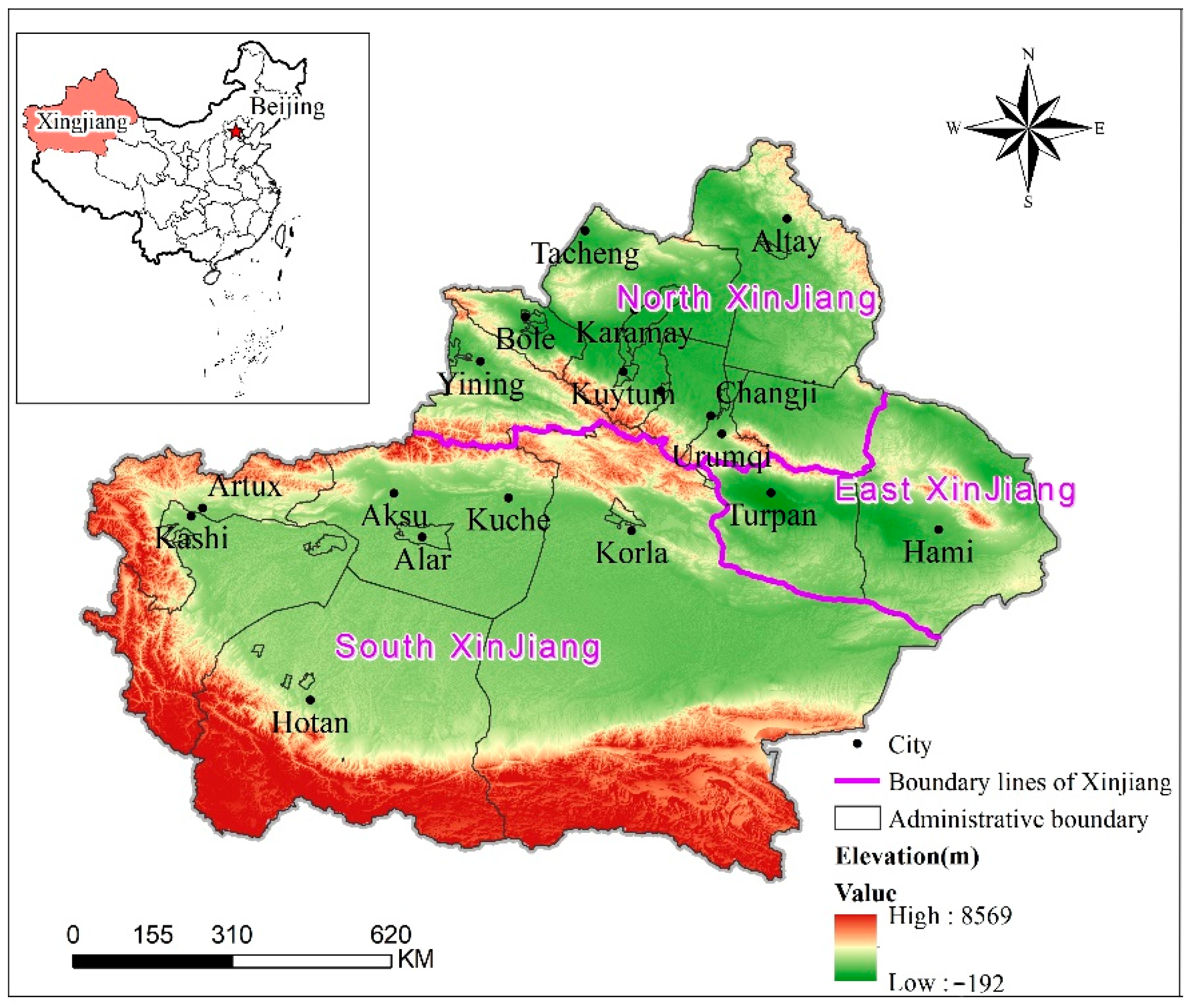
2.1. Study Site Description

The XJ region is located in northwestern China. It is located in the hinterland of the Eurasian continent, with a geographic position of 34°09′ N~49°08′ N, 73°25′ E~96°24′ E. The XJ region is characterized by an extensive distribution of mountains, deserts, oases, glaciers, and snow [21]. The study area covers an area of about 1.66 × 10⁶ km2. There are 14 regions, namely Urumqi, Altay, Bozhou, Changji, Karamay, Tacheng, Yili, Aksu, Bazhou, Kashgar, Hotan, Kexu, Hami, and Turfan. The geographical factors of the Tianshan Mountains and the human factors of XJ have also divided these regions into the northern, southern, and eastern border areas (Figure 1) [22]. XJ is far from the ocean and has a temperate continental arid climate, with average annual hours of sunshine of about 2800 h. The average annual evaporation potential ranges from 1600 mm to 2300 mm, which is much more than the average annual precipitation (157.4 mm) [23]. The total water resources of XJ in 2020 were 83.16 × 10⁹ m3, of which 78.77 × 10⁹ m3 were surface water resources, 50.35 × 10⁹ m3 were underground water resources, and 45.96 × 10⁹ m3 were double-counted between surface water and underground water. Its local primary industry (agriculture, forestry, animal husbandry, and fishery) production water consumption was 49.61 × 10⁹ m3, which dominated (93.4%) in its total water consumption (53.11 × 10⁹ m3) [24].

2.2. Meteorological, Water Resource, and Statistical Data Sources

The basic data for this study included meteorological data, water resource data, and statistical data, of which the meteorological data (precipitation, air temperature, average wind speed, sunshine hours, and relative humidity) were obtained from the data of 88 meteorological stations provided by the China Meteorological Data Sharing Service Network (http://data.cma.cn/, accessed on 1 August 2021). The hydrological data (water resources, primary industry water consumption, domestic water consumption, and total water consumption) were obtained from the XJ Water Resources Bulletin (2001–2020) provided by the Water Resources Bureau of XJ Uygur Autonomous Region. The statistical data (resident population number, GDP, value added of CNY 10,000 of industry, cultivated area, meat production of livestock, fertilizer application, etc.) were obtained from the XJ Statistical Yearbook (2001–2021) and the XJ Production and Construction Corps Statistical Yearbook (2001–2021) provided by the XJ Bureau of Statistics and XJ Production and Construction Corps Bureau of Statistics.

2.3. Methodology

2.3.1. Agricultural Water Footprint

In this study, based on the water footprint theory of Hoekstra [25] and others, we calculated the agricultural water footprint ( A W F ) in XJ, including the crop water footprint ( W F c r o p ) and the animal water footprint ( W F a n i m a l ). The calculation formula is as follows:
AWF = W F c r o p + W F a n i m a l
where A W F is the agricultural water footprint (m3); W F c r o p is the crop water footprint (m3); and W F a n i m a l is the animal water footprint (m3).
(1)
Crop Water Footprint
The water footprint of crops is the amount of water resources consumed by crops in the course of their growth. Depending on the type of water consumed and its impact on the environment, it can be further classified into a blue water footprint, green water footprint, or gray water footprint, which are calculated using the following formulas:
W F c r o p = W F c r o p - b l u e + W F c r o p - g r e e n + W F c r o p - g r e y
where W F c r o p is the water footprint of the crops (m3); W F c r o p - b l u e is the blue water footprint of the crops (m3); W F c r o p - g r e e n is the green water footprint of the crops (m3); and W F c r o p - g r e y is the gray water footprint of the crops (m3).
In this paper, major crops were selected for the water footprint calculation based on the XJ Uygur Autonomous Region Statistical Yearbook and the XJ Production and Construction Corps Statistical Yearbook. The crops included 15 crops such as rice, wheat, coarse cereals, soybeans, cotton, oil plants, sugar beets, vegetables, melons, potatoes, alfalfa, grapes, apples, fragrant pears, and red jujube. According to the statistics, it can be seen that the selected crops accounted for 88.7% of the total cultivated area in XJ. Therefore, in this paper, the sum of the water footprints of the above 15 crops was taken as the blue–green water footprint of the crops in XJ. Firstly, this paper calculated the evapotranspiration ( E T c ) and effective rainfall ( P e f f ) during the reproductive period of each major crop in the study area. The Penman–Monteith method, recommended by the Food and Water Agriculture Organization of the United Nations (FAO), was used to calculate E T c (mm), which can accurately calculate E T c under different regions and climatic conditions [26]. P e f f (mm) was calculated using the CROPWAT model recommended by the FAO. Secondly, the blue water footprint and green water footprint of the different crops in each region were calculated separately based on the source of water use using the formulas shown below [27]:
W F c r o p - b l u e = 10 × l g p d = 1 m a x ( 0 , E T c P e f f ) / Y × P i
W F c r o p - g r e e n = 10 × l g p d = 1 m i n ( E T c , P e f f ) / Y × P i
where P i is the total yield (t) of crop i . Y refers to the crop yield per unit area (t/ha). Coefficient 10 is a coefficient for converting water depth into water volume per unit area of land area. is the cumulative amount of blue (or green) water from the planting period to the harvesting period. l g p is the length of the growing season (d).
The gray water footprint of crops mainly refers to the amount of water required to dilute underutilized fertilizer to its standard concentration after its application through leaching it into rivers via irrigation water or rainfall, which produces polluting ions. In this paper, we analyzed the gray water footprint of the crops using nitrogen and phosphorus fertilizers, which are the most applied in XJ, as the main sources of polluting ions. The same water body can dilute multiple pollutants at the same time, so the gray water footprint is determined by the amount of water required to dilute the largest pollutant ion. The calculation formula is shown below [28]:
W F c r o p - g r e y = m a x ( α T N × L n i t - f e r C m a x T N C m i n T N , α T P × L p h o - f e r C m a x T P C m i n T P )
where α T N , α T P are the fertilizer loss coefficients of nitrogen and phosphate fertilizers, respectively, taken from the First National Pollution Source Census–Manual of Fertilier Loss Coefficients of Agricultural Pollution Sources; L n i t - f e r , L p r o - f e r are the discounted pure application amounts (kg) of the nitrogen fertilizer and phosphate fertilizer, respectively; C m a x T N and C m a x T P are the maximum concentrations of pollutants if TN and TP reach the environmental water quality standards; C m a x T N = 0.01 kg·m−3, taken from the US EPA standards; C m a x T P = 0.005 kg·m−3; and C m i n T N and C m i n T P are the initial concentrations of TN and TP in the receiving water body, assumed to be 0.
(2)
Animal Water Footprint
The animal water footprint is defined as the water footprint of each animal throughout its life cycle from birth to slaughter, including water consumed in the form of virtual and direct water for growth, processed feed, drinking water, and washing services, calculated using the formula shown below [29]:
W F a n i m a l = W F a n i f e e d + W F a n i d r i n k + W F a n i s e r v e
where W F a n i m a l is the animal water footprint (m3); W F a n i - f e e d is the animal feed water footprint (m3); W F a n i - d r i n k is the animal drinking water footprint (m3); and W F a n i - s e r v e is the animal service water footprint (m3).
In this paper, the main animal products were selected according to the XJ Uygur Autonomous Region Statistical Yearbook and the XJ Production and Construction Corps Statistical Yearbook for the purposes of the water footprint calculation. The animal products included cattle, horses, camels, pigs, goats, sheep, chickens, and rabbits; these comprised eight categories of livestock, using live animal data to remove the growth and feed processing water used and the overlap with the water footprint of the feed crops. The calculation of the formula is shown in the following equation [30]:
W F a n i f e e d = b i r t h d e a t h Q m i x + i = 1 N S W C i × C i j d t
W F a n i d r i n k = b i r t h d e a t h Q d i d t
W F a n i s e r v e = b i r t h d e a t h Q s i d t
where Q m i x denotes the amount of water required for mixed feed (m3·d−1); C i j is the weight of feed j consumed by the ith animal (t·d−1); and S W C j denotes the amount of virtual water contained in feed i (m3·t−1). The virtual water volume of the feed crops was calculated using the crop water footprint method, weighted according to the ration (weight) of different feed crops; Q d i and Q s i are the amount of water required as drinking water and for washing services for animal i per day (m3·d−1), respectively.

2.3.2. Water Resource Pressure Assessment Index

The water resource pressure index ( W R P I ) reflects the degree of pressure on regional water resources, characterizing the load on water resources from human production and living processes and the relative scarcity of regional water resources. In order to explore the actual pressure on the water resources in each region of XJ, the actual consumption of water resources was measured based on the results of regional water footprint calculations, and the ratio of the actual consumption of regional water resources ( A W F ) to the total water resources in a broad sense ( W A a l l ) was used to express the pressure on the water resources. The calculation formula is shown below:
W R P I = A W F / W A a l l
where WRPI is the water resource stress index; AWF is the total water footprint of regional agricultural production (m3); and W A a l l is the total water resources of the region in a broad sense (m3). When WRPI > 1, that means that the water consumption of agricultural production has exceeded the amount of available water resources, and the larger the value, the more serious the local water resource pressure; similarly, when WRPI ≤ 1, the smaller the value, the smaller the water resource pressure.

2.3.3. Exploratory Spatial Data Analysis

Exploratory spatial data analysis (ESDA) is a method used to analyze spatial data and express them visually, which can intuitively reveal characteristics of spatial data such as their correlation, aggregation, and hot/cold spots [31]. Global spatial autocorrelation is usually chosen to characterize the spatial correlation of the geographic phenomena across an entire region, which reflects the overall trend in the spatial correlation of the observed variables across the whole study area. The commonly used measure is global Moran’s I statistic, and the I statistic index takes a value between −1 and 1. The formula is shown below [32]:
I = N S 0 i = 1 N j = 1 N W i j ( X i X ) ( X j X ) j = 1 N ( X i X ) 2
where i j , N is the number of study objects; X i is the observation; X ¯ is the mean value of X i ;   S 0 = i = 1 N j = 1 N W i j ; and W i j is the spatial weighting matrix between the study objects i and j , with a spatial proximity of 1 and non-proximity of 0.
Although global spatial autocorrelation analysis can reveal the degree of dependence on objects as a whole, it ignores possible local smoothing; therefore, local spatial autocorrelation must be chosen to reveal the autocorrelation of the local regional units in the neighboring space and to reflect the degree of spatial agglomeration of a certain element in detail, which is represented by a LISA agglomeration map. In this paper, local Moran’s I index was used to measure the heterogeneity of the spatial elements between the regional units i and j , and the calculation formula is shown below [33]:
I i = Z i i = 1 n W i j Z j
where Z i and Z j are the normalization of the observations in spatial cells i and j , respectively; and W i j is the spatial weight.

2.3.4. Logarithmic Mean Divisia Index

Logarithmic Mean Divisa Index (LMDI) decomposition is a complete, residual-free decomposition analysis method part of the Divisia index method [34]. Its core idea is to decompose a target variable into a combination of several influencing factor changes so that the magnitude of the influence of each factor can be identified, and then the factors that contribute more can be determined [35]. Based on the research purpose of exploring the drivers of agricultural water footprint changes in XJ, this paper decomposed them into a population effect (pop-eff), life effect (life-eff), structural effect (struc-eff), scale effect (scale-eff), technology effect (tech-eff), economic effect (econ-eff), ecological effect (ecol-eff), and environmental effect (env-eff). Among them, pop-eff shows the change in p i j , life-eff shows the change in l i j , struc-eff shows the change in s t i j , scale-eff shows the change in s c i j , tech-eff shows the change in T i j , econ-eff shows the change in e c o n i j , ecol-eff shows the change in e c o l i j , and env-eff exhibits the change in e n v i j . According to the LMDI full decomposition model, the formulas for each factor effect are shown below [36,37]:
p o p - e f f i = j = 1 14   ω f i j ln p j t p j 0
l i f e - e f f i = j = 1 14   ω f i j ln l j t l j 0
s t r u c - e f f i = j = 1 14   ω f i j ln s t j t s t j 0
s c a l e - e f f i = j = 1 14   ω f i j ln s c j t s c j 0
t e c h - e f f i = j = 1 14   ω f i j ln T j t T j 0
e c o n - e f f i = j = 1 14   ω f i j ln e c o n j t e c o n j 0
e c o l - e f f i = j = 1 14   ω f i j ln e c o l j t e c o l j 0
e n v - e f f i = j = 1 14   ω f i j ln e n v j t e n v j 0
s t j = A W j   T W j  
T j = Y j   T W j  
e c o n j = Y j   p j  
ω f i j = W F i j t W F i j 0 ln W F i j t ln W F i j 0
Δ WF = pop - eff + life - eff + struc - eff + scale - eff + ( tech - eff ) + ( econ - eff ) + ( ecol - eff ) + ( env - eff )
where ω f i j denotes the weight; p j denotes the population of j area (104); l j denotes the domestic water consumption of j area (108 m3); s c j denotes the area of crop cultivation in j area (103 ha); e n v j denotes the natural oasis area in j area (km2); e n v j denotes the total carbon dioxide emissions of j area (104 t); A W j denotes the agricultural water use in j region (m3); T W j denotes the total water use in j region (m3); Y j denotes the gross domestic product in j region (CNY 104); and “ΔWF” denotes the change in the water footprint of agriculture in XJ. The superscripts “0” and “t” denote the base year and target year of this study, respectively.

2.3.5. Geographical Detector

A geoprobe is a spatial statistical method used to explore the degree of influence of geographic factors on the spatial differentiation of a geographic phenomenon and to analyze the causes of such differentiation. In this paper, the factor detection part is used to explore the influence of different factors on the spatial distribution of water stress in XJ’s prefectures and cities. The formula for calculating the degree of influence of geographic factors is shown below [38]:
q = 1 h = 1 L N h σ h 2 N σ 2
where q is the value of the degree of influence of influencing factors on water stress in XJ; h = 1, 2, …; L is the classification number of the influencing factors; N is the number of prefectural and municipal administrative divisions in XJ; N h denotes the number of prefectural and municipal administrative regions classified as h ; σ 2 is the variance in the interstate water stress index in XJ’s prefectures; and σ h 2 is the variance in the regional water stress index classified as h . The value of q is [0, 1], and the larger the value of q is, the greater the influence of this factor on water stress in XJ. q = 0 means that it is not affected by this factor.

3. Results

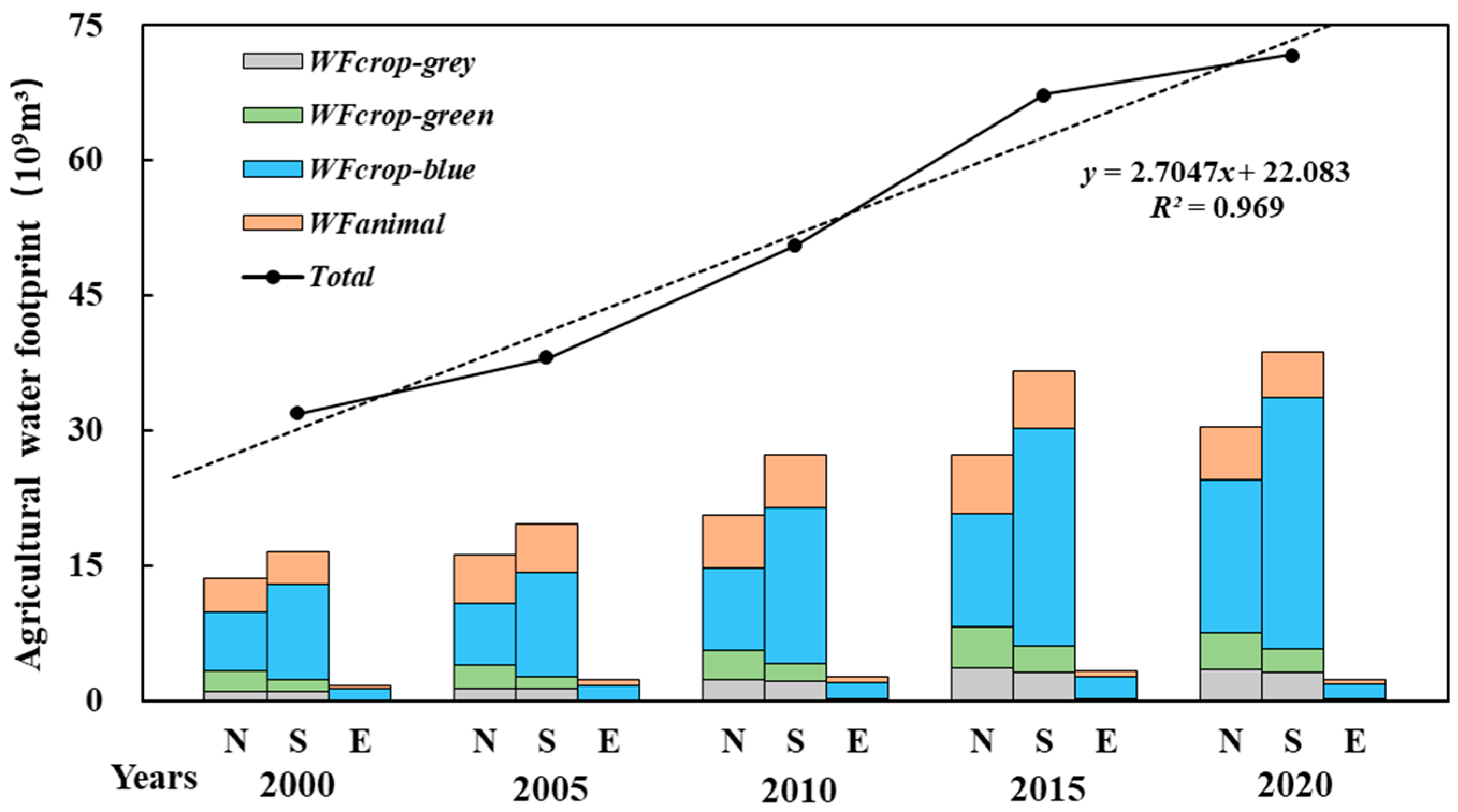
3.1. Temporal Evolution Analysis of the Agricultural Water Footprint

Figure 2 depicts the trend in XJ’s agricultural water footprint ( A W F ) from 2000 to 2020. The results show that the total A W F increased by 124.0% over the past 20 years ( W F c r o p and W F a n i m a l increased by 147.9% and 48.9%, respectively). The regional differences in the annual average value of A W F were obvious; in order from highest to lowest are the southern border (27.74 × 10⁹ m3), the northern border (21.67 × 10⁹ m3), and the eastern border (2.43 × 10⁹ m3). Among them, the A W F at the southern border was 11.42 times higher than that at the eastern border.
In the agricultural production process, the W F a n i m a l multi-year average was 22.4 per cent of the A W F multi-year average, so it can be seen that W F c r o p is a major component of A W F (~77.6%). Of the three components that make up W F c r o p in each region, blue water dominates (74.6%), with relatively small proportions of green water (14.0%) and gray water (11.4%). Similar to W F c r o p , W F c r o p - b l u e showed a gradual increase in all zones from 2000 to 2020, with the southern border contributing the most to the components of W F c r o p - b l u e (60.0%), followed by the northern border (34.2%) and the eastern border (5.8%). Compared with W F c r o p - b l u e ,the interannual changes in W F c r o p - g r e e n and W F c r o p - g r e y showed an overall relatively small increase in all regions.

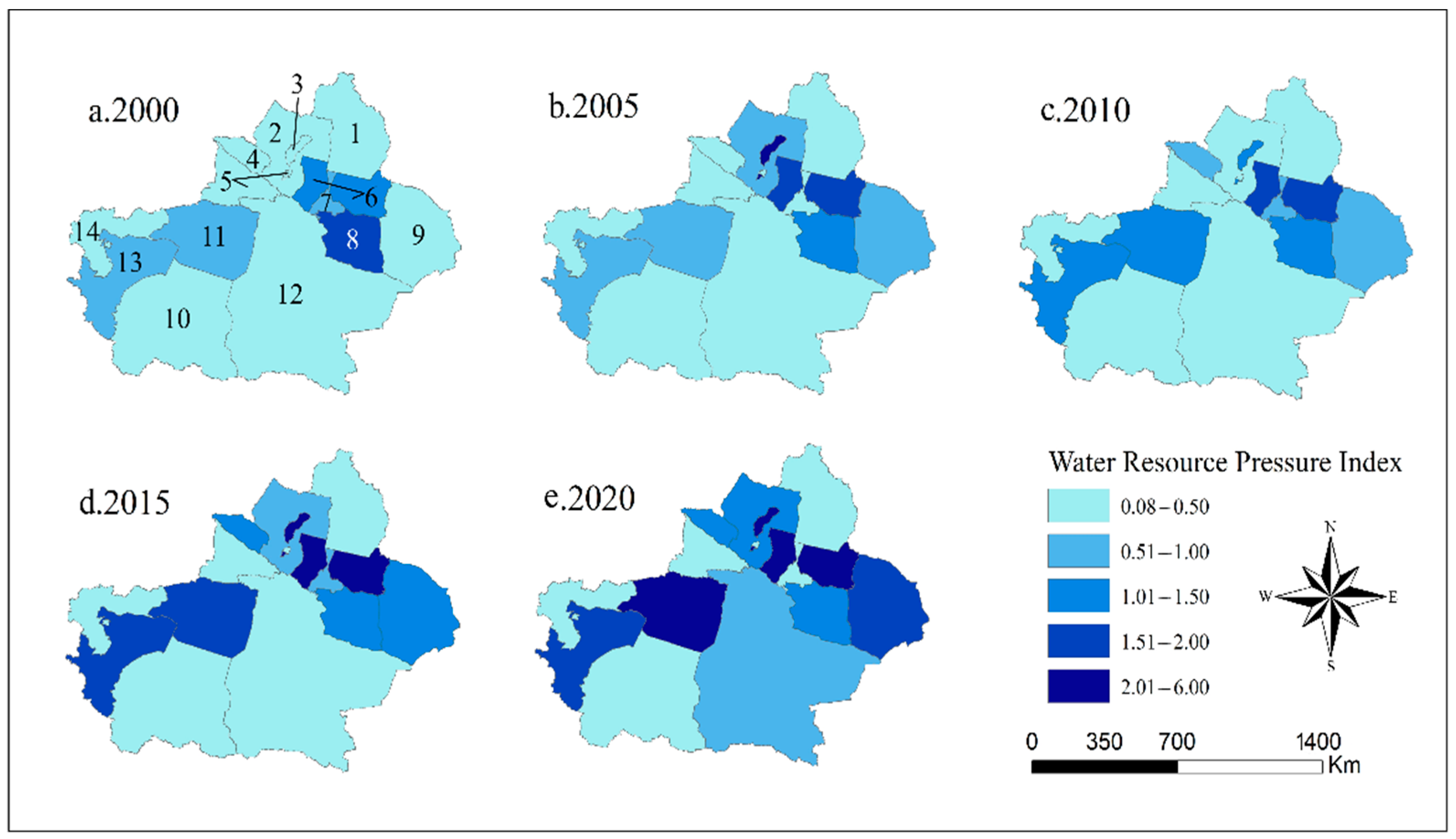
3.2. Spatio-Temporal Evolution Analysis of Water Resource Pressure

We calculated the water resource pressure index (WRPI) for each prefecture in XJ from 2000 to 2020. In this paper, due to space limitations, we only selected data for 2000, 2005, 2010, 2015, and 2020 to map the changes in the spatial patterns of the WRPI according to five levels, as follows: lower (0.08 ≤ WRPI < 0.5), low (0.51 ≤ WRPI < 1.0), medium (1.01 ≤ WRPI < 1.5), high (1.51 ≤ WRPI < 2.0), and higher (2.01 ≤ WRPI < 6.0) (Figure 3).
With the development of the social economy and the intensification of the frequency of human water extraction activities, the overall water stress in XJ has shown an increasing trend year by year (Figure 3). The results show that from 2000 to 2020, the water resource pressure index increased by 187.1%. Among them, water resources in Turpan (1.83) were under high pressure in 2000, followed by Changji (1.19), Kashgar (0.68), and Aksu (0.53), while the rest of the region had a low water resource pressure index, and the pressure index at the junction of eastern and northern XJ was relatively high. In 2005, the water stress in Karamay (increased by 1.75) and Tacheng (increased by 0.23) increased more than in previous years, resulting in a relatively high stress index in the northern border area; meanwhile, in the southern border area, the situation remained the same as in 2000. In 2010, the stress index increased in Bortala, Urumqi, Aksu, and Kashgar, and the water stress eased in Karamay and Tacheng. In this period, the water stress was higher in both the eastern (1.04) and southern (0.51) regions than in the northern region (0.37). In 2015, the water resource pressure in southern XJ, northern XJ, and eastern XJ had increased to varying degrees compared to the previous period, and this increase in pressure was also mainly characterized in the different prefectures mentioned above. By 2020, water stress in XJ had increased rather than decreased, reaching the strongest stress level (0.89) in the past 20 years. All regions had indices higher than 1.0 except for the six prefectures of Altay, Urumqi, Ili, Kizilsu, Hotan, and Bayingol, which had relatively low stress levels, with the highest WSI in Karamay (5.82) and the second and third highest being Changji (3.45) and Aksu (2.19), respectively. Overall, over the last 20 years, the WSI in the eastern XJ region has generally been higher than that in the southern and northern XJ regions, while the Karamay, Changji, and Aksu regions have been the regions with higher WSIs among the many prefectures of XJ.

3.3. Spatial Correlation Analysis of Water Resource Pressure

3.3.1. Global Spatial Autocorrelation Analysis of Water Resource Pressure in XJ

The global Moran’s I index and significance level p-value were calculated based on a neighborhood queen spatial weight matrix for the 2000, 2005, 2010, 2015, and 2020 time cross-section data. This revealed the spatial clustering/dispersion of the water stress indices in XJ’s prefectures and cities in the last 20 years. The calculated Moran’s I and p-values were 0.1089 (p = 0.0428), −0.2851 (p = 0.0042), −0.2109 (p = 0.0032), −0.3301 (p = 0.0025), and −0.3258 (p = 0.0029). These results indicate that the water stress index of XJ’s prefecture and municipalities passed the 95% confidence interval assumption within the period from 2000 to 2005, but the Moran index was relatively small, and the spatial positive autocorrelation effect was relatively insignificant. Within the period from 2005 to 2020, the Moran index was less than 0, indicating its negative spatial autocorrelation, i.e., water stress had obvious discrete spatial characteristics. In 2000–2005 and 2010–2015, the degree of aggregation was weakened, and the discrete nature was increasing; meanwhile, in 2005–2010 and 2015–2020, the degree of aggregation was enhanced, and the discrete nature was slightly weakened. There were clear fluctuations in dispersion across the study periods, with the sharpest fluctuations occurring between 2000 and 2005.

3.3.2. Local Spatial Autocorrelation Analysis of Water Resource Pressure in XJ

In order to reveal the discrete spatial phenomenon of water resource pressure in each province, LISA clustering maps of the water resource pressure in XJ in 2000, 2005, 2010, 2015, and 2020 were plotted based on the local Moran’s I index and a Moran scatterplot (Figure 4). The results of LISA plots are often categorized into High–High Cluster (H-H), Low–Low Cluster (L-L), High–Low Cluster (H-L), Low–High Cluster (L-H), and not significant, where the HH and LL types both exhibit a spatially positive correlation type. The HL and LH types both exhibit spatially negative correlation types, and not significant indicates no obvious clustering or discrete features. In the blocks of five-year periods, 6, 5, 4, 3, and 3 prefecture cities and municipalities were in a state of spatial positive/negative correlation (HH, HL, or LH clustering), respectively. Overall, they followed a decreasing trend, and the change trend was the same as the G-Moran’s I trend, indicating that the discrete spatial status of water resource pressure in XJ’s cities and towns showed an intensifying trend over time. In 2005 and 2010, the HH agglomeration was consistent, and in the remaining years, only one prefecture experienced HH agglomeration. In 2000, two prefectures had an HL concentration. For 2005–2020, there was only one geographic area with HL agglomeration. The number of prefectures with LH agglomeration was the largest in those five years, decreasing gradually from three prefectures in 2000 to one prefecture in 2020.
The water stress HH catchment area is mainly located at the junction of the eastern and northern borders, principally including the cities of Turpan and Urumqi, forming an area with high values for the water stress index. The region began to expand in 2005 and then shrunk to only one place in 2015, mainly due to a shortage of precipitation, which resulted in high water stress. This has become a resource shortcoming in the process of socio-economic development. Water stress HL agglomeration is mainly distributed in the western part of the southern border, and there are only a few prefectures in this state of water stress, including Kashgar and Aksu in 2000; meanwhile, only Kashgar remained in the HL agglomeration state after 2005. Water stress LH agglomeration is scattered throughout XJ, with Altay, Tacheng, and Bayingol in this state in 2000; then, Altay, Tacheng, and Bayingol transformed from this state to a discrete state in sequence in the next 5 to 15 years until 2020, when only Hami, which is adjacent to Turpan, was transformed from a discrete state to an LH agglomeration state. Over the past 20 years, with the transformation of agglomeration–disagglomeration states among XJ’s prefectures, water stress agglomeration has weakened, and fluctuations in disagglomeration have increased. Moreover, the number of spatially correlated prefectures has decreased, the resource mismatch has increased, and the differences in the water resource background conditions and water use between prefectures have gradually become larger.

3.4. Analysis of Factors Influencing the Evolution of the Production Water Footprint and Water Resource Pressure

Considering the comprehensive and accessible nature of the data, four influencing factors, comprising people’s lives, agricultural development, economy and technology, and the ecological environment, were selected, including the following relationships between effects: a total population–population effect (X1); a domestic water consumption–life effect (X2); a proportion of agricultural water consumption–structure effect (X3); a cultivation area–scale effect (X4); a water consumption of CNY 10,000 GDP–technology effect (X5); a GDP per capita—economic effect (X6); a natural oasis area—ecological effect (X7); and a total carbon dioxide emissions—environmental effect (X8). The LMDI method was used to decompose the contribution rate of each factor to the change in the water footprint, and the geoprobe method was used to explore the factors influencing the regional differences in XJ’s water stress index and analyze the intensity of their roles.

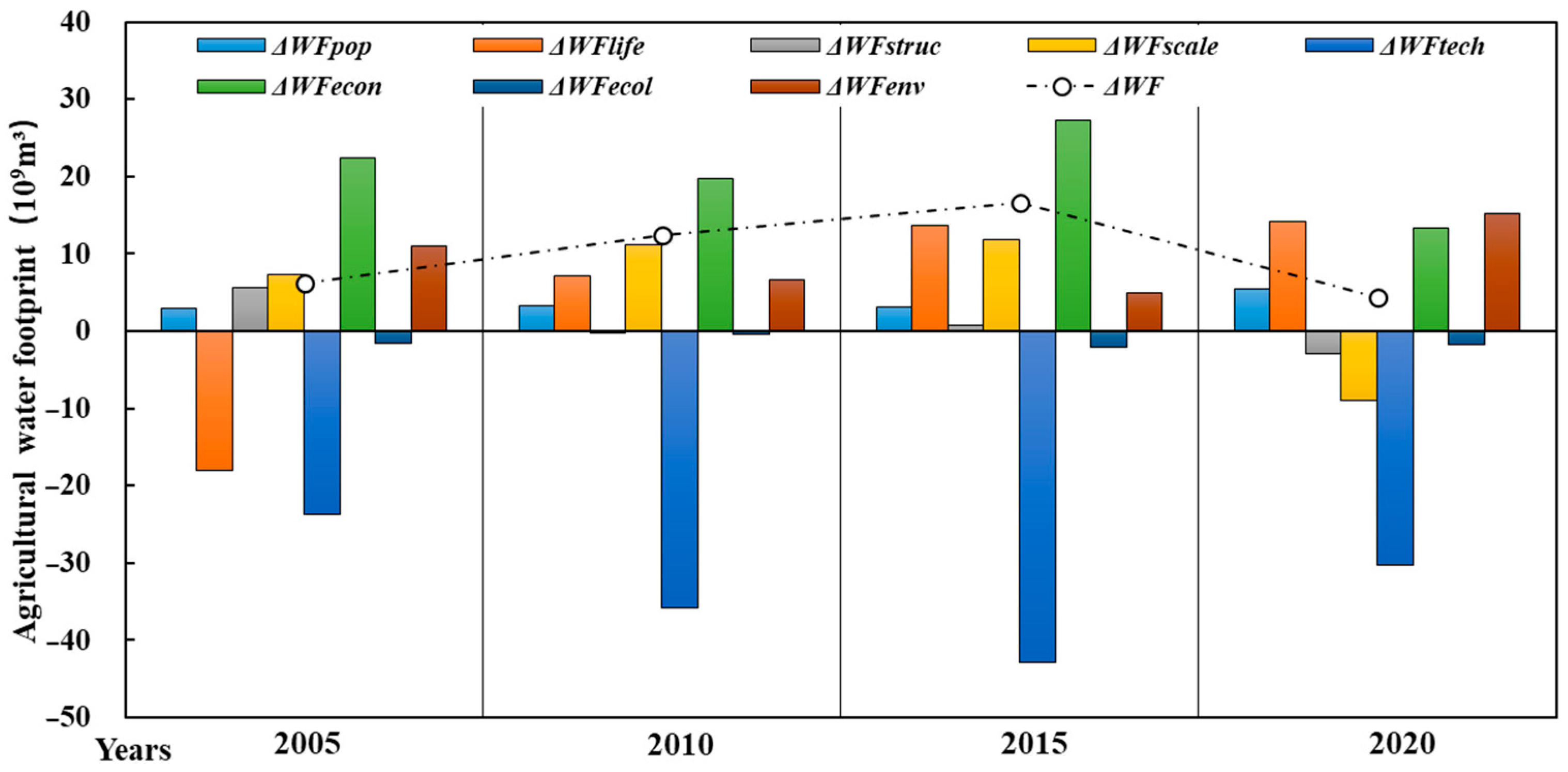
3.4.1. Contribution Value of the Agricultural Water Footprint’s Driving Factors in XJ

In order to further explore the factors influencing the agricultural water footprint in XJ, the contribution value of each driver of the water footprint in XJ was calculated with 2000 as the base year and 5 years as the time period (Figure 5). The total effect of each factor in XJ from 2005 to 2020 has always been positive, but the overall trend has declined, and 2015 was the turning point for the trend in the total value of the total effect. From a structural point of view, the absolute value of the share of each factor in the amount of change in the agricultural water footprint is as follows, in descending order: technical effect (−3.35) > economic effect (2.09) > environmental effect (0.95) > scale effect (0.54) > life effect (0.43) > population effect (0.37) > ecological effect (−0.14) > structural effect (0.09). Among them, the technology effect and economic effect accounted for a much larger proportion than the contributions of the other factors, with mean values of −33.15 × 10⁹ m3 and 20.70 × 10⁹ m3, respectively. Among the many factors, the economic effect, the environmental effect, and the population effect have always promoted the growth of the agricultural water footprint; on the contrary, the technology effect and the ecological effect always inhibit it, while the life effect, the structure effect, and the scale effect play different individual roles in the growth of the water footprint at different stages. Overall, the influence of the technology and economic effects dominates the process of growth in the agricultural water footprint in XJ.
The population effect of the change in the agricultural water footprint in XJ generally ranges from 3.01× 10⁹ to 5.38 × 10⁹ m3, showing a fluctuating upward trend; this indicates that although the population effect has had a relatively small impact on the growth of the water footprint in XJ, it has always played a facilitating role. The livelihood effect was a reverse driver of the water footprint’s growth before 2005 but became a facilitator after 2005, with an average annual contribution of 4.21 × 10⁹ m3 to the agricultural water footprint. As with the population effect, the livelihood effect has had a relatively small impact on the water footprint changes in XJ. Among the many factors, the structure effect has had the smallest impact on the change in the agricultural water footprint in XJ, with an average annual contribution value of only 0.9 × 10⁹ m3. This indicates that although there have been changes in the water use structure in XJ, their overall effect is not obvious. The scale effect is similar to the livelihood effect, which positively drove the water footprint before 2015 but inhibited it after 2015. The average contribution of the scale effect to the changes in XJ’s agricultural water footprint declined most significantly overall, by −2.2 percent. The technology effect has driven the increase in XJ’s agricultural water footprint in the reverse direction. The average annual contribution of the technology effect to the water footprint from 2005 to 2020 was as high as −33.15 × 10⁹ m3, with a mean contribution value of −335%. This indicates that the efficiency of water use in XJ improved across the period, and water resources were developed and utilized in a more intensive and efficient way than in the base period. The economic effect is the main factor that has caused the growth in the agricultural water footprint in XJ. The economic effect was a positive driver from 2005 to 2020, with an average annual contribution value of 20.7 × 10⁹ m3 and a mean contribution value of 209%. In addition, it is the higher share and rapid growth of the economic effect that has caused the total water footprint of XJ to continue to show an upward trend despite the continuous improvements in water use efficiency. The ecological effect is generally in the range of −0.33 × 10⁹~−2.02 × 10⁹ m3, which means it has not played an obvious role; however, in the same way as the technological effect, the ecological effect has always inhibited the growth of the agricultural water footprint in XJ. The environmental effect shows a fluctuating upward trend in the period 2005–2020, with an average annual contribution of 9.44 × 10⁹ m3 to the growth in the agricultural water footprint, contributing 95% of the mean value. This makes it the third most influential factor after the technological and economic effects.

3.4.2. Intensity of Factors Influencing Water Resource Pressure in XJ

Firstly, the natural breakpoint method was applied to divide the eight indicators into 10 levels, and then geodetic factor detection was used to calculate the intensity of the role of each indicator (q-value) in order to obtain the calculation results (Table 1). The main indicators affecting the spatial differentiation of the water stress index did not change significantly in different periods; however, the intensity of the role of each indicator factor changed significantly. Among them, the indicator with the highest-intensity role in the spatial differentiation of the water resource pressure in XJ was the cultivated area (0.665) in 2000, and per capita GDP (0.223) had the lowest-intensity role in the same year. Over time, each indicator showed an increasing or decreasing trend in the overall intensity of its effect on the spatial differentiation of water resource pressure during the 20-year period. The indicators showing an increasing trend in descending order were domestic water use (135.3%) > GDP per capita (93.7%) > total CO2 emissions (29.2%) > area of natural oases (9.4%). Meanwhile, the indicators showing a decreasing trend in descending order were water use per CNY 10,000 of GDP (−18.8%) > total population (−10.3%) > share of water used in agriculture (−2.4%) > area under cultivation (−0.2%).
In 2000, specifically, the most important factor contributing to the spatial differentiation of water stress was the area under cultivation, followed by the total population and then the proportion of water used in agriculture, with GDP per capita playing the weakest role. In 2005, the main factor shifted from the area under cultivation to the total population, with the intensity of the area under cultivation decreasing over the five-year period after 2005, while the intensity of the natural oasis areas increased significantly, and the intensity of total CO2 emissions was the lowest in the same year. In 2010, identical to the position in 2000, the cultivated area was still the most important factor, while the intensity of domestic water consumption was significantly higher than the other factors. The intensity of the population, agricultural water use, and natural oasis area had decreased significantly, and the weakest-intensity role was played by GDP per capita. In 2015, the cultivated area was slightly more important than it had been five years previously, and the factors with an intensity greater than 0.6 were oasis area, domestic water use, and agricultural water use, with CO2 emissions having the lowest intensity. In 2020, although the intensity index had decreased slightly, the main influencing factor was still the planted area, while the intensity of total CO2 emissions had risen significantly and was one of the top three factors, together with natural oasis areas and planted areas, and the intensity of water consumption per CNY 10,000 GDP reached its lowest value in 20 years and was also the weakest factor in that year.
In conclusion, although the main factors affecting the spatial differentiation of water stress have shifted between cultivated areas and population in recent years, it is undeniable that the intensity of the effect of cultivated areas on the spatial differentiation of water stress has remained high over the past 20 years. In addition to the number of people, the proportion of agricultural water use and the area of natural oases continue to have a greater impact on the spatial differentiation of water stress. In general, for XJ, the expansion of its irrigation scale, its population growth, the imbalance of the industrial (water use) structure, and the evolution of natural–artificial oases had the greatest influence on the spatial differentiation of water stress, while GDP per capita had the weakest influence, followed by water use per CNY 10,000 GDP.

4. Discussion

4.1. Key Factors Affecting Changes in the Agricultural Water Footprint and Water Stress and Suggestions for Addressing Them

As shown by the historical development trend, A W F shows a continuous growth trend in terms of spatial and temporal changes ( W F c r o p and W F a n i m a l are also in these states). If corresponding regulatory policies are not implemented, the growth of W F c r o p - b l u e , driven through the expansion of the cultivation area and irrigation scale, will lead to a reduction in natural oasis areas, which will further lead to the obvious decline in biohabitat quality, water productivity, and the carbon sequestration capacity of vegetation [39]. On the other hand, an increase in agricultural fertilizer’s application, due to W F c r o p - g r e y ’s growth, will not only place enormous pressure on water use for the dilution of hazardous chemicals, affecting the surface and groundwater quality to some extent, but will also cause a deterioration in soil quality and a decline in crop yields due to the continued accumulation of salts in the soil [40]. If there is a decline in the marginal effects of the objective input costs (e.g., agricultural mechanization and cropping systems, etc.), the scale of agricultural (plantation and livestock) production in XJ will expand further. Therefore, from the perspective of sustainable development in the future, the government has proposed policies to address this issue in order to maintain an appropriate scale of agricultural development. Under this policy, W F c r o p - b l u e , W F c r o p - g r e y , and W F a n i m a l will decrease with the gradual implementation of the policy. In addition, in future sustainable development scenarios, the government should pay special attention to the phenomenon of the erosion of natural oases through the growth of artificial oases, and avoiding the severity of this phenomenon as much as possible will effectively improve the problem of deteriorating habitat quality. Existing studies have shown that the implementation of such management measures can increase the overall ecosystem service value of the region [41,42].
The industrial development of the XJ region is dominated by agriculture, and thus agricultural water use occupies a pivotal position in the process of water use for socio-economic development in XJ [43]. The impact of the share of agricultural water use on water stress in XJ is significant, and thus an accurate evaluation of agricultural water use in XJ’s states is fundamental to the evaluation of water stress. The use of water footprinting methods to assess agricultural water use efficiency and water stress has been widely adopted worldwide [44]. However, it has been demonstrated during the development and utilization of existing water resources that the implementation of water-saving technologies will improve the water use efficiency of decision-makers; however, the development of water-saving irrigation systems, the optimization of water allocation in irrigation districts, and the development of irrigation water demand forecasting technologies may lead to a continued high level of socio-ecological water demand and use, a further crowding-out of natural vegetation, and increased water consumption by water bodies, thus illustrating the “Jevons paradox” of water saving applied in the agricultural context [45].
The degree of the match between irrigation water use and the distribution pattern of effective irrigated areas is one of the most important indicators affecting the water stress index. The amount of water resources consumed throughout the economic production process in XJ is more closely related to the scale of crop cultivation in terms of time and space. Thus, we believe that the most effective way to rationally and optimally allocate water and alleviate water stress would be to focus on the spatial matching of water and land resources and their sensitivity [46]. In short, water resource management policy-makers can alleviate the structural imbalance between water resources and land resources through measures such as promoting the transfer of agricultural land and changing the scale of agricultural land management, thereby alleviating the existing water resource pressure across XJ. On the other hand, in terms of cropping structure, farmers in all regions of XJ tend to grow cash crops (e.g., cotton and jujube) rather than food crops in order to maintain their smooth income and standard of living. As a result, the large-scale production of high water-consuming cash crops further increases the pressure on local water resources, so it is important to encourage farmers to increase the proportion of low-water-consuming crops and to grant or increase subsidies to farmers.
Therefore, in the implementation of future development policies, the government should focus on China’s “One Belt, One Road” initiative to optimize and develop the product structure of the processing and service industries, and through adjustments to the industrial structure, it can effectively reduce the ineffective consumption of water resources and ensure the high-quality development of the socio-economics of the whole region, so as to achieve a win-win situation [47]. From a macro perspective, governors should pay more attention to improving agricultural production while maintaining a benign ecological environment, developing better resource carrying capacity assessment tools to accurately assess the appropriate carrying capacity of each region, and improving the integrated management of water and land resources [48]. From an engineering perspective, the government can alleviate the current imbalance between agricultural development and water use through the implementation of inter-regional water transfer projects and integrated planning for planting scale control, thereby reducing the water stress index.

4.2. Discussion on the Driving Mechanism of Agricultural Water Footprint and Water Resource Pressure

Through this study and analyses of its drivers, we have obtained preliminary results that explore the spatial evolution trend in the agricultural water footprint, water stress, and its main drivers in XJ from 2000 to 2020. Firstly, the three major factors that make the highest contribution to the change in the agricultural water footprint in XJ are the technological effect, the economic effect, and the environmental effect. Among them, the technological effect plays an inhibiting role, while the economic and environmental effects have instead positively driven the growth in the water footprint. Secondly, the three most important factors contributing to the spatial differentiation in water stress in XJ are the cultivated areas, the natural oasis areas, and the agricultural water use ratio. Although the intensity of these drivers has been quantified, the mechanisms driving the spatial evolution of water stress are not yet fully understood.
The emergence and evolution of anything are closely related to its original developmental basis. New water stress patterns generally represent the inheritance and development of existing patterns. Therefore, the basis of historical development is one of the main driving mechanisms for the differences in water stress among XJ’s states. From 2000 to 2020, although there was a certain degree of randomness and instability in the spatial distribution of the water resource pressure across XJ, the overall trend showed that it was concentrated in the western part of the southern border and the border between the eastern and northern parts of the border. One of the reasons for this is that the prefecture and municipalities in this region have always been constrained by its water resource conditions in various ways, such as the degree of development of its irrigation districts, the characteristics of its industrial structure, and obvious disadvantages in terms of water vapor’s abundance and scarcity.
Regional geography is one of the important factors that influences the evolution of regional water stress patterns. Through its influences on the sequence of and opportunities for regional water resource development, it is related to the development speed of regional water resource development and utilization and the status of the local spatial autocorrelation of water pressure. From 2000 to 2015, in terms of the spatial autocorrelation of the water resource pressure differences between the cities and towns in XJ, HL agglomeration and LH agglomeration were always mainly concentrated in the southern XJ region, and regional water resources development and use perform relatively poorly in terms of overall correlation. The ecological environment of the southern border region is relatively fragile, the degree of exploitation and utilization has gradually increased but in a more relaxed manner, and the main water resource background conditions do not have any significant disadvantages compared with those of the northern border. However, the sufficient and positive conditions for crop cultivation and production have led to the rapid development of the scale of agricultural irrigation in the southern XJ region, and its industrial structure is far less reasonable than that in other regions of XJ. This has further led to a massive outflow of local physical water resources to the rest of the country in the form of virtual water, resulting in an inefficient economic use of resources and ultimately creating a significant gap between the pressure on water resources, the competitive environment of economic development, and the dynamism of economic development here in comparison with other regions.
Regional development policy is an important driving force in the evolution of regional water stress differentials and plays a very important role in shaping regional water stress patterns. In a sense, regional development policy actually reflects a specific priority, which is the government’s intention and goals for regional development, i.e., balanced or unbalanced regional development, formed after comprehensive research and analysis. From 2001 to 2010, the state proposed the Western Development Strategy, and XJ was one of the key regions in the implementation of this strategy because it was rich in resources but its people’s income level was generally low [49]. After the 16th Party Congress in 2002, the Party Central Committee and the State Council agreed that XJ’s development required national input and thus implemented a series of poverty alleviation programs and deployments focusing on farmland water conservancy in XJ. However, this directly contributed to the growth in crop acreage, and the significant increase in the agricultural water footprint has further increased the proportion of water used in agriculture, exacerbating the difficult water resource carrying situation. After 2010, the implementation of the XJ aid policy further enabled XJ in its growth and development from a previously weak industrial base. With the support of other provinces across the country, its development has been further focused on arable land reclamation and comprehensive agricultural development, especially in the southern XJ region, in the form of constructing water-efficient zones and developing eco-agricultural demonstration parks [50]. Up to the present day, the effect of such policy factors on the formation of spatial patterns in water resource use continues to be amplified.

5. Conclusions

This paper took the XJ region as a case study. Working from the perspective of its agricultural water footprint, the regional water stress index was accounted for in the results of an agricultural water footprint assessment based on the past 20 years. Trend analysis and ESDA were applied to analyze the characteristics of the spatial pattern evolution and spatial correlation of the water stress index in XJ’s prefectures and cities from 2000 to 2020. The LMDI and geodetectors were used to detect the factors influencing the evolution in the agricultural water footprint and the spatial differentiation in water stress, respectively. The conclusions are as follows:
(1)
From 2000 to 2020, XJ’s agricultural water footprint was in a state of continuous growth, with the total amount more than doubling. Among the components of the agricultural water footprint, the crop water footprint increased more than the animal water footprint, and significant growth has occurred mainly in the southern and northern regions. During the study period, changes in the water stress in XJ’s cities and towns were unstable, with super-high water stress indices concentrated in the eastern XJ region, and the overall trend was upward. The spatial distribution of the water stress index was uneven, concentrated in the west and east of XJ, and the regional differences between the north and the south were smaller than those between the east and the west. Regions such as Karamay, Changji, Turpan, Aksu, and Kashgar had high multi-year average water stresses.
(2)
The spatial correlation of the water resource pressure index is obvious, its negative correlation is significant, and the intensity of the discrete state shows fluctuating changes. The water resource pressure HH agglomeration area is mainly concentrated in the junction zone of east XJ and north XJ, and the HL agglomeration area is mainly distributed in the western part of south XJ; however, the spatial changes in these two agglomerations were relatively small, while the changes in the LH agglomeration area were larger. During the period of 2000–2020, the state of water resource pressure agglomeration in XJ weakened, the fluctuation of the discrete state was enhanced, the number of spatially correlated prefectures decreased, the mismatch continued to increase, and the differences were gradually highlighted. Therefore, the XJ government should pay more attention to the variability in the water stress between regions to avoid increasing polarization.
(3)
In terms of its contribution to driving the change in the agricultural water footprint in XJ, the total effect of each factor was always positive during the period of 2005–2020, but the effect value generally showed a downward trend. Among them, 2015 was the turning point for the change in the trend in the total effect value, in which the technological effect (water consumption of CNY 10,000 GDP), the economic effect (GDP per capita), and the environmental effect (total carbon emission of CO2) had the most significant impact on the evolution of the agricultural water footprint in XJ. Therefore, the government should formulate policies to encourage the innovation and development of agriculture-related technologies. In this way, it can promote the suppression of technological effects on the agricultural water footprint, thereby reducing water stress in XJ. The intensity of the effect of different factors on the spatial differentiation of the water stress index in XJ was not the same in different time periods. The spatial differentiation of water resources in XJ has mainly been determined by the expansion of its irrigation scale (cultivated area), the growth of its population (total population), the imbalance of its industrial structure (share of agricultural water use), and the evolution of the area of natural oases.
This study can provide new perspectives for further analyzing the actual state of the water footprint and water stress in XJ and provide a reference basis for decision-makers in the XJ government. Future research in this field should pay more attention to the following aspects: firstly, the spatial matching of the agricultural water footprint and land resources and their sensitivity; secondly, accurate assessment of a suitable regional carrying capacity and development of the assessment tools; thirdly, feasibility studies on reducing water stress through integrated planning of transregional water transfer projects and cultivation scale control.

Author Contributions

Conceptualization, C.R.; methodology, J.Y. and A.L.; software, C.R.; validation, X.D., J.Z., Y.W., S.W. and A.L.; formal analysis, X.L.; investigation, C.R.; resources, A.L.; data curation, S.W.; writing—original draft preparation, C.R.; writing—review and editing, P.Z.; visualization, J.Y.; supervision, X.D., Y.W. and A.L.; project administration, J.Z. and X.L.; funding acquisition, X.D., J.Y. and S.W. All authors have read and agreed to the published version of the manuscript.

Funding

This work was financially supported by the National Natural Science Foundation of China (Grant No. 52379020; Grant No. 52179028; Grant No. 52309041; Grant No. 72304245).

Data Availability Statement

The original contributions presented in this study are included in the article; further inquiries can be directed to the corresponding author.

Conflicts of Interest

Author Shuhong Wang was employed by the company Xinjiang Corps Survey and Design Institute (Group) Co., Ltd. The remaining authors declare that the research was conducted in the absence of any commercial or financial relationships that could be construed as a potential conflict of interest.

References

  1. Zarei, Z.; Karami, E.; Keshavarz, M. Co-production of knowledge and adaptation to water scarcity in developing countries. J. Environ. Manag. 2020, 262, 110283. [Google Scholar] [CrossRef] [PubMed]
  2. Zhang, L.; Yu, Y.; Ireneusz, M.; Malgorzata, W.; Sun, L.; Yang, M.; Wang, Q.; Yu, D. Water Resources Evaluation in Arid Areas Based on Agricultural Water Footprint—A Case Study on the Edge of the Taklimakan Desert. Atmosphere 2022, 14, 67. [Google Scholar] [CrossRef]
  3. Feng, K.; Hubacek, K.; Pfister, S.; Yu, Y.; Sun, L. Virtual scarce water in China. Environ. Sci. Technol. 2014, 48, 7704–7713. [Google Scholar] [CrossRef] [PubMed]
  4. Jiao, L. Food security. Water shortages loom as northern China’s aquifers are sucked dry. Science 2010, 328, 1462–1463. [Google Scholar] [CrossRef] [PubMed]
  5. Piao, S.; Fang, J.; Zhou, L.; Ciais, P.; Zhu, B. Variations in satellite-derived phenology in China’s temperate vegetation. Glob. Chang. Biol. 2006, 12, 672–685. [Google Scholar] [CrossRef]
  6. Dai, Y.Y. Quantitative Evaluation of Generalized Water Resources in Changing Environment Based on Water Cycle Simulation. Master’s Thesis, China University of Mining and Technology, Xuzhou, China, 2019. [Google Scholar]
  7. Falkenmark, M.; Widstrand, C. Population and water resources: A delicate balance. Popul. Bull. 1992, 47, 1–36. [Google Scholar] [CrossRef] [PubMed]
  8. Gabriela, A.; Antonio, M.M.; Edson, T. Assessing sectoral water stress states from the demand-side perspective through water footprint dimensions decomposition. Sci. Total Environ. 2021, 809, 152216. [Google Scholar] [CrossRef]
  9. Liu, X.; Du, H.; Zhang, X.; Feng, K.; Zhao, X.; Zhong, H.; Zhang, N.; Chen, Z. Assessing Transboundary Impacts of Energy-Driven Water Footprint on Scarce Water Resources in China: Catchments under Stress and Mitigation Options. Environ. Sci. Technol. 2023, 57, 9639–9652. [Google Scholar] [CrossRef]
  10. Pfister, S.; Koehler, A.; Hellweg, S. Assessing the environmental impacts of freshwater consumption in LCA. Environ. Sci. Technol. 2009, 43, 4098–4104. [Google Scholar] [CrossRef]
  11. Gai, L.; Xie, G.; Li, S.; Cheng, Y.; Luo, Z. The Analysis of Water Footprint of Production and Water Stress in China. J. Resour. Ecol. 2016, 7, 334–341. [Google Scholar] [CrossRef]
  12. Zeng, Z.; Liu, J.; Savenije, H.H.G. A simple approach to assess water scarcity integrating water quantity and quality. Ecol. Indic. 2013, 34, 441–449. [Google Scholar] [CrossRef]
  13. Jia, X.; Yan, Y.; Zhu, C.; Bai, X.; Hu, M.; Wu, G. Approaches for Regional Water Resources Stress Assessment: A Review. J. Nat. Resour. 2016, 31, 1783–1791. [Google Scholar] [CrossRef]
  14. Zeng, D.; Wang, J.; Li, Y.; Jiang, J.; Lv, L. Spatial-temporal Variation of Water Resources Stress and Its Influencing Factors Based on Water-saving in China. Sci. Geogr. Sin. 2021, 41, 157–166. [Google Scholar] [CrossRef]
  15. Sun, S.; Wu, P.; Wang, Y.; Zhao, X.; Liu, J.; Zhang, X. The impacts of interannual climate variability and agricultural inputs on water footprint of crop production in an irrigation district of China. Sci. Total Environ. 2013, 444, 498–507. [Google Scholar] [CrossRef] [PubMed]
  16. Zhao, X.; Zhao, J.; Ma, C.; Xiao, L.; Ma, C.; Wang, X. Study of resource-environmental pressure considering the Footprint Family in Yunnan Province, China. Acta Ecol. Sin. 2016, 36, 3714–3722. [Google Scholar] [CrossRef]
  17. Chapagain, A.K.; Hoekstra, A.Y. The blue, green and grey water footprint of rice from production and consumption perspectives. Ecol. Econ. 2011, 70, 749–758. [Google Scholar] [CrossRef]
  18. Fan, L.; Wang, H.; Liu, C.; Sui, G. Vulnerability assessment of water resources based on pressure-state-response model in Xinjiang. South-To-North Water Transf. Water Sci. Technol. 2022, 20, 1052–1064. [Google Scholar] [CrossRef]
  19. Zhang, L.; Deng, X.; Long, A.; Gao, H.; Ren, C.; Li, Z. Spatia-temporal assessment of water resource security based on the agricultural water footprint: A case in the Hotan Prefecture of Xinjiang. Arid Zone Res. 2022, 39, 436–447. [Google Scholar] [CrossRef]
  20. Feng, Z.H. Research on the Evaluation of Agricultural Sustainable Development in Northwest China Based on Water Resources Carrying Capacity. Ph.D. Thesis, Xi’an University of Technology, Xi’an, China, 2021. [Google Scholar]
  21. Yao, J.; Zhao, Y.; Chen, Y.; Yu, X.; Zhang, R. Multi-scale assessments of droughts: A case study in Xinjiang, China. Sci. Total Environ. 2018, 630, 444–452. [Google Scholar] [CrossRef]
  22. Hai, Y.; Long, A.; Zhang, P.; Deng, X.; Li, J.; Deng, M. Evaluating agricultural water-use efficiency based on water footprint of crop values: A case study in Xinjiang of China. J. Arid Land 2020, 12, 580–593. [Google Scholar] [CrossRef]
  23. Zhang, Q.; Sun, P.; Li, J.; Singh Vijay, P.; Liu, J. Spatiotemporal properties of droughts and related impacts on agriculture in Xinjiang, China. Int. J. Climatol. 2015, 35, 1254–1266. [Google Scholar] [CrossRef]
  24. Xiniiang Uygur Autonomous Region Statistics Bureau. Xinjiang Statistical Yearbook; China Statistics Press: Beijing, China, 2020. [Google Scholar]
  25. Hoekstra, A.Y. Water Footprint Assessment: Evolvement of a New Research Field. Water Resour. Manag. 2017, 31, 3061–3081. [Google Scholar] [CrossRef]
  26. Yu, J.; Long, A.; Deng, X.; He, X.; Zhang, P.; Wang, J.; Hai, Y. Incorporating the red jujube water footprint and economic water productivity into sustainable integrated management policy. J. Environ. Manag. 2020, 269, 110828. [Google Scholar] [CrossRef]
  27. Hoekstra, A.Y.; Chapagain, A.K.; Aldaya, M.M.; Hoekstra, M.M.M. The Water Footprint Assessment Manual: Setting the Global Standard; Routledge: London, UK, 2011. [Google Scholar]
  28. Cui, S.; Dong, H.; Wilson, J. Grey water footprint evaluation and driving force analysis of eight economic regions in China. Environ. Sci. Pollut. Res. Int. 2020, 27, 20380–20391. [Google Scholar] [CrossRef] [PubMed]
  29. Zhang, P.; Deng, M.; Long, A.; Deng, X.; Wang, H.; Hai, Y.; Wang, J.; Liu, Y. Coupling analysis of social-economic water consumption and its effects on the arid environments in Xinjiang of China based on the water and ecological footprints. J. Arid Land 2020, 12, 73–89. [Google Scholar] [CrossRef]
  30. Chapagain, A.K.; Hoekstra, A.Y. Virtual Water Flows between Nations in Relation to Trade in Livestock and Livestock Products; IHE Delft: Delft, The Netherlands, 2003. [Google Scholar]
  31. Shekhar, S.; Xiong, H.; Zhou, X. Encyclopedia of GIS; Springer: Cham, Switzerland, 2017. [Google Scholar]
  32. Qin, W.; Wang, L.; Xu, L.; Sun, L.; Li, J.; Zhang, J.; Shao, H. An exploratory spatial analysis of overweight and obesity among children and adolescents in Shandong, China. BMJ Open 2019, 9, e028152. [Google Scholar] [CrossRef] [PubMed]
  33. Cheniti, H.; Cheniti, M.; Brahamia, K. Use of GIS and Moran’s I to support residential solid waste recycling in the city of Annaba, Algeria. Environ. Sci. Pollut. Res. Int. 2021, 28, 34027–34041. [Google Scholar] [CrossRef]
  34. Ang, B.W. Decomposition analysis for policymaking in energy: Which is the preferred method? Energy Policy 2004, 32, 1131–1139. [Google Scholar] [CrossRef]
  35. Ang, B.W.; Xu, X.Y.; Su, B. Multi-country comparisons of energy performance: The index decomposition analysis approach. Energy Econ. 2015, 47, 68–76. [Google Scholar] [CrossRef]
  36. Papagiannaki, K.; Diakoulaki, D. Decomposition analysis of CO2 emissions from passenger cars: The cases of Greece and Denmark. Energy Policy 2009, 37, 3259–3267. [Google Scholar] [CrossRef]
  37. Zhao, C.; Chen, B. Driving Force Analysis of the Agricultural Water Footprint in China Based on the LMDI Method. Environ. Sci. 2014, 48, 12723–12731. [Google Scholar] [CrossRef]
  38. Wang, G.; Peng, W. Quantifying spatiotemporal dynamics of vegetation and its differentiation mechanism based on geographical detector. Environ. Sci. Pollut. Res. Int. 2022, 29, 32016–32031. [Google Scholar] [CrossRef] [PubMed]
  39. Gong, B.; Liu, Z. Assessing impacts of land use policies on environmental sustainability of oasis landscapes with scenario analysis: The case of northern China. Landsc. Ecol. 2020, 36, 1913–1932. [Google Scholar] [CrossRef]
  40. Balasubramaniam, T.; Shen, G.; Esmaeili, N.; Zhang, H. Plants’ Response Mechanisms to Salinity Stress. Plants 2023, 12, 2253. [Google Scholar] [CrossRef]
  41. Zhang, Z.; Xia, F.; Yang, D.; Huo, J.; Wang, G.; Chen, H. Spatiotemporal characteristics in ecosystem service value and its interaction with human activities in Xinjiang, China. Ecol. Indic. 2020, 110, 105826. [Google Scholar] [CrossRef]
  42. Wang, Y.; Zhang, S.; Zhen, H.; Chang, X.; Shataer, R.; Li, Z. Spatiotemporal Evolution Characteristics in Ecosystem Service Values Based on Land Use/Cover Change in the Tarim River Basin, China. Sustainability 2020, 12, 7759. [Google Scholar] [CrossRef]
  43. Zhang, P.; Deng, X.; Long, A.; Hai, Y.; Li, Y.; Wang, H.; Xu, H. Impact of Social Factors in Agricultural Production on the Crop Water Footprint in Xinjiang, China. Water 2018, 10, 1145. [Google Scholar] [CrossRef]
  44. Mekonnen, M.M.; Hoekstra, A.Y. Water footprint benchmarks for crop production: A first global assessment. Ecol. Indic. 2014, 46, 214–223. [Google Scholar] [CrossRef]
  45. Wang, Y.; Long, A.; Xiang, L.; Deng, X.; Zhang, P.; Hai, Y.; Wang, J.; Li, Y. The verification of Jevons’ paradox of agricultural Water conservation in Tianshan District of China based on Water footprint. Agric. Water Manag. 2020, 239, 106163. [Google Scholar] [CrossRef]
  46. Long, A.; Yu, J.; Deng, X.; He, X.; Du, J. Understanding the Spatial-Temporal Changes of Oasis Farmland in the Tarim River Basin from the Perspective of Agricultural Water Footprint. Water 2021, 13, 696. [Google Scholar] [CrossRef]
  47. Gao, D.; Long, A.; Yu, J.; Xu, H.; Zhao, X. Assessment of Inter-Sectoral Virtual Water Reallocation and Linkages in the Northern Tianshan Mountains, China. Water 2020, 12, 2363. [Google Scholar] [CrossRef]
  48. Vanham, D.H.; Hoekstra, A.Y.; Wada, Y.; Bouraoui, F.; de Roo, A.; Mekonnen, M.M.; van de Bund, W.J.; Batelaan, O.; Pavelic, P.; Bastiaanssen, W.G.M.; et al. Physical water scarcity metrics for monitoring progress towards SDG target 6.4: An evaluation of indicator 6.4.2 “Level of water stress”. Sci. Total Environ. 2018, 613–614, 218–232. [Google Scholar] [CrossRef] [PubMed]
  49. Pu, C.; Quan, L. Reflections on the Development of the West and the Anti-Poverty Problem in Xinjiang. J. Xinjiang Univ. Financ. Econ. 2000, 4, 5–6. [Google Scholar]
  50. Long, A.; Zhang, P.; Hai, Y.; Deng, X.; Wang, J. Spatio-Temporal Variations of Crop Water Footprint and Its Influencing Factors in Xinjiang, China during 1988–2017. Sustainability 2020, 12, 9678. [Google Scholar] [CrossRef]
Figure 1. The topographic map of XJ, including north XJ, south XJ, and east XJ.
Water 16 01164 g001
Figure 2. Recent trends in agricultural water footprint in each district of the XJ. North XJ (abbreviated as N); south XJ (S); east XJ (E).
Water 16 01164 g002
Figure 3. The spatial pattern of water resource pressure index in XJ from 2000 to 2020 (ae). 1. Altay Prefecture (abbreviated as Altay); 2. Tacheng Prefecture (Tacheng); 3. Karamay City (Karamay); 4. Bortala Mongolian Autonomous Prefecture (Bortala); 5. Ili Kazak Autonomous Prefecture (Ili); 6. Changji Hui Autonomous Prefecture (Changji); 7. Urumqi City (Urumqi); 8. Turpan City (Turpan); 9. Hami Prefecture (Hami); 10. Hotan Prefecture (Hotan); 11. Aksu Prefecture (Aksu); 12. Bayingol Mongolian Autonomous Prefecture (Bayingol); 13. Kashgar Prefecture (Kashgar); 14. Kizilsu Kirgiz Autonomous Prefecture (Kizilsu).
Water 16 01164 g003
Figure 4. A LISA cluster map of water resource pressure in XJ from 2000 to 2020 (ae).
Water 16 01164 g004
Figure 5. The contribution value of water footprint’s driving factors in XJ.
Water 16 01164 g005
Table 1. The effect intensity of each influencing factor in different years.
YearX1X2X3X4X5X6X7X8
20000.6190.2320.5770.6650.2820.2230.5660.473
20050.6410.5590.5990.6340.5500.3850.6160.387
20100.5270.6140.5640.6630.4060.2520.5030.569
20150.5170.6010.6000.6640.4110.4060.6260.356
Disclaimer/Publisher’s Note: The statements, opinions and data contained in all publications are solely those of the individual author(s) and contributor(s) and not of MDPI and/or the editor(s). MDPI and/or the editor(s) disclaim responsibility for any injury to people or property resulting from any ideas, methods, instructions or products referred to in the content.

