The Three-Dimensional Wave-Induced Current Field: An Analytical Model

Abstract

Wave-induced currents play a critical role in coastal dynamics, influencing sediment transport and shaping bottom topography. Traditionally, long- and cross-shore currents in coastal zones were analyzed independently, often with two-dimensional models for longshore currents and undertow being used. The introduction of quasi-three-dimensional models marked a significant advancement toward a more holistic understanding. Despite recent proposals for fully three-dimensional models, none have achieved widespread acceptance, primarily due to challenges in accurately capturing depth-dependent radiation stress. This paper presents an innovative analytical model advocating for comprehensive three-dimensional approaches in coastal hydrodynamics. The model, based on novel simplification rules, refines relationships governing turbulent stress tensors and provides valuable insights into wave-induced stresses. It offers analytical solutions for both homogeneous and general coastal zones, laying the foundation for future advancements in numerical modeling techniques.

1. Introduction

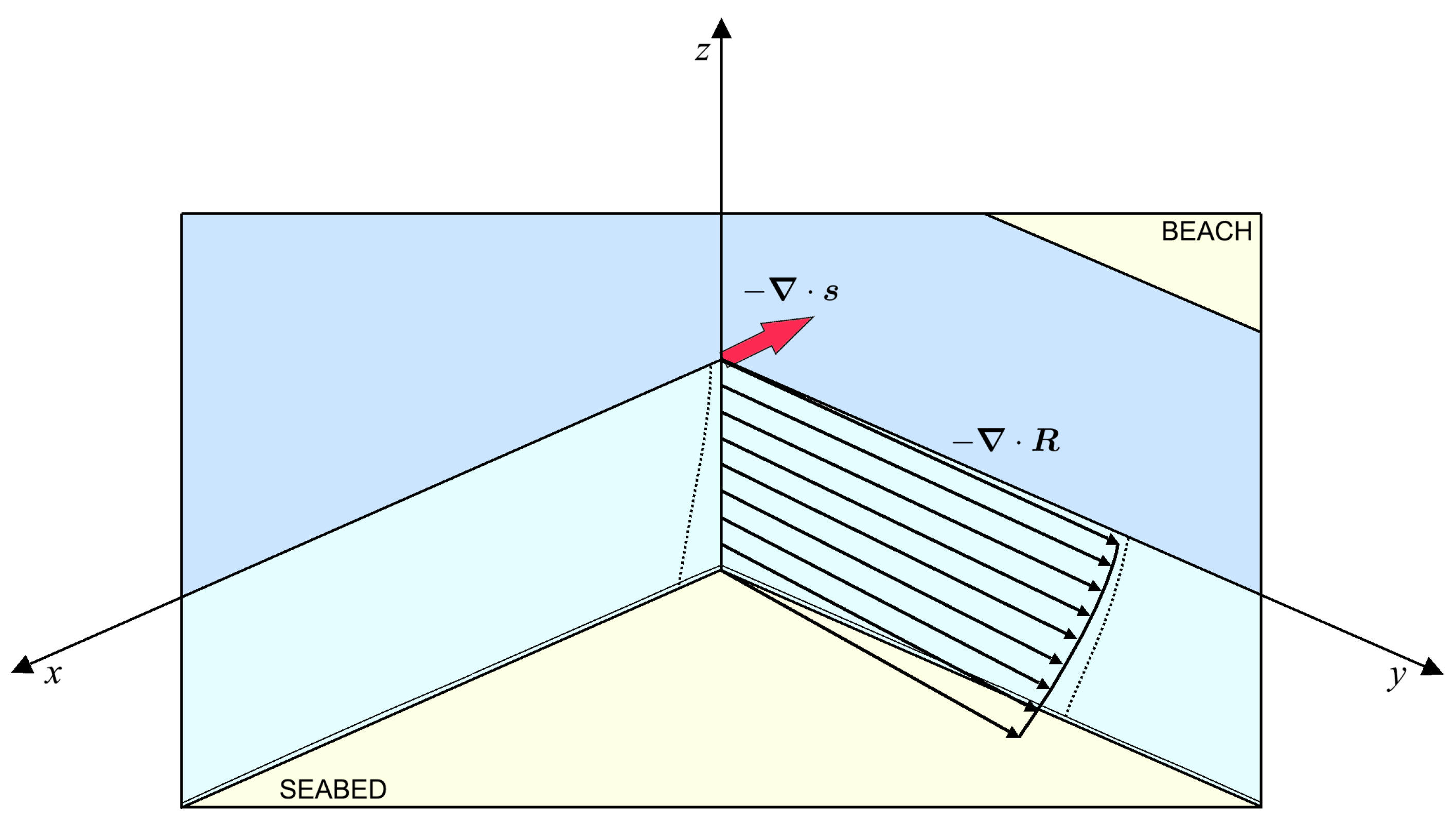
Wave-induced currents play an important role in the dynamics of coastal zones dominated by wave activity, serving as a crucial mechanism for transferring energy from the atmosphere to the ocean and eventually to the seabed. Among these currents, the undertow and longshore currents stand out due to their significant contributions to the movement of bedload and, alongside wave-generated orbital velocities and turbulent movements near the seabed, to changes in the coastal zone bottom topography. Consequently, understanding these currents is essential for predicting erosional and accumulative processes in coastal zones, as well as for addressing key issues related to coastal protection and ensuring the safety of ships near ports. To gain a complete understanding of wave-induced currents, a full three-dimensional study is required, as this is the only method capable of accounting for all components influencing the velocity field within the coastal zone. Figure 1 illustrates the three-dimensional mean velocity distribution within the coastal zone.

Historically, the main currents within coastal zones, including both long- and cross-shore currents, have been analyzed independently. Since the early seventies, two-dimensional models for these currents have been established, with longshore currents modeled based on depth-integrated radiation stress and the undertow driven by the imbalance between the average depth-dependent momentum flux induced by surface waves and the slope of an average position of the water surface, described by the radiation stress [1,2,3].

By the late 1980s, the requirement for a three-dimensional representation of wave-induced current fields had been identified, prompting the creation of quasi-three-dimensional models [4]. These models attempted to combine separate models of longshore currents and undertow to offer an approximate spatial distribution of the flow (see, e.g., [5,6]). Despite the popularity of these models in the 1990s, their reliance on two-dimensional solutions meant that in certain scenarios, such as within the coastal zone of a small island, the resulting velocity field could significantly deviate from reality.

A comprehensive understanding of wave-induced currents in coastal zones necessitates a three-dimensional approach, ensuring the integration of all influencing elements into the flow dynamics. However, the primary challenge in developing such models lies in identifying depth-dependent radiation stress, which serves as the driving force behind these currents. Several attempts have been made to address this challenge. For instance, Nobuoka et al. [7] introduced a novel three-dimensional nearshore current model, incorporating key concepts such as the variability of onshore and offshore flow and a sole reliance on wave motion as the driving force. Mellor’s ([8,9,10]) research contributed to advancing comprehensive models integrating three-dimensional current dynamics and surface wave interactions, offering a holistic understanding of ocean dynamics.

Additionally, Kumar et al. [11] aimed to enhance three-dimensional radiation stress formulations to improve the accuracy of predicting wave-induced currents and rip currents in the surf zone. Chou et al. [12] focused on developing and applying a three-dimensional numerical model coupling wave dynamics with hydrodynamics in South San Francisco Bay, aiming to understand the complex interactions in the Bay Area. Ranasinghe [13] concentrated on developing advanced numerical models to simulate interactions between waves and submerged structures under regular waves, ultimately aiming to enhance the understanding of wave interactions in such scenarios.

It is worth noting that machine learning is rapidly advancing and being applied across various disciplines, including coastal zone hydrodynamics (see, e.g., [14]). However, it faces several limitations that currently hinder the successful description and resolution of wave-induced currents.

In terms of analytical model formulation, Xia et al. [15] focused on the vertical variation of radiation stress, providing insights into its depth-dependent changes and its influence on the generation and behavior of wave-induced currents. Additionally, an alternative formulation based on the Dirac delta function, presented by Kołodko and Gic-Grusza [16], offers a simplified and concise description of the vertical variability of excess horizontal momentum flux due to wave presence, presenting a novel approach to the analytical modeling of wave-induced currents. Chybicki [17] also contributed significantly to this discourse by extending the original concept of radiation stress in water waves to encompass its vertical variation, achieving a precise delineation of radiation stress density alongside straightforward computational formulas for assessing the vertical radiation stress profile. This work parallels the foundational principles posited by Dolata and Rosenthal [18], albeit with a more refined expression for the pressure function. The discourse on radiation stress theory was further elaborated by Mellor [19], who engaged in a comparative analysis between the concepts of “radiation stress” and “vortex force.” In this work, Mellor advocates for the Longuet-Higgins ([1,2]) and Mellor ([8,20]) theoretical framework, critiquing the “vortex force” theory as extended by McWilliams and Restrepo [21] and addresses the inaccuracies present in research based on the vortex force concept. The significance of radiation stresses within coastal zones was reaffirmed in Mellor’s subsequent work [22], reinforcing their critical role in coastal dynamics.

The foundation of the research presented in this paper is anchored by numerous hypotheses, primarily focusing on the methodology for constructing the model’s underlying equations. Central to contemporary hydrodynamics are the momentum transport equations (the Navier–Stokes equations), accompanied by the mass transport Equation (the continuity equation). However, it has become increasingly clear that transforming these equations into a structure that facilitates the creation of an exhaustive three-dimensional model for wave-induced currents in coastal areas poses substantial challenges and is yet to be fully accomplished.

Traditionally, the description of the flows in question utilized the wave period-averaged mass transport equation (see, for example, Svendsen and Lorenz [23]; Nobuoka and Mimura [24]). However, some authors did not adequately consider the necessity of integrating this equation before its averaging (see, for example, Lee and Wang [25]; Smith [26]), resulting in a misinterpretation of the equations and, consequently, as observed by Cieślikiewicz and Gudmestad [27], the omission of the wave transport on the averaged free surface, i.e., the area between the wave crest and trough. The work presented here assigns crucial importance to this area, both in terms of mass and momentum transport. It seems that without accounting for the processes occurring on the averaged free surface, it is not feasible to meaningfully define the quasi-turbulent stress tensor (or, alternatively, quasi-Reynolds stress tensor), which acts as a local force-generating flow.

The main assumptions and hypotheses of this work are as follows:

• A consistent assumption that all terms of higher order than the square of the wave amplitude are negligibly small. This leads, among other things, to the exclusion from the model of wave–current and current–current interactions (unlike, for example, the work of Svendsen and Putrevu [28], in which certain terms of the order of the square of the wave amplitude, a, are omitted, while others—of the order of $a^4$—are retained).
• The assumption is made that for the problem at hand, it is sufficient to apply the theory of small amplitude waves to describe wave motion. This is a widely accepted practice based on which, for instance, the components of the radiation stress tensor are defined. However, the applicability of this assumption is not suitable for the surf-zone area. A further consequence of adopting linear wave theory in this work is the omission of the average value of products of orthogonal components of wave velocities (i.e., the product of horizontal velocity components with the vertical component), whose role is emphasized in the literature (see, for example, Rivero and Arcilla [29]). For the same reason, the so-called "roller", defined as a mass of water moving between the crest and trough of a breaking wave at phase speed (see, e.g., [30]), which attempts to account for wave nonlinearity in the coastal zone, is also omitted. However, it is worth noting that Svendsen and Lorenz [23] estimated the contribution of the roller to the obtained flow velocity values at only 9%, somewhat justifying its exclusion in the prototype version of the constructed three-dimensional model.
• A new, simplified constitutive relationship defining turbulent stresses specifically for the coastal zone is proposed. To date, turbulence in this area has been poorly understood (see, for example, [31]). Therefore, the most straightforward approach to modeling the considered stresses using turbulent viscosity coefficients (according to the Boussinesq hypothesis) was chosen. However, taking into account the specifics of the coastal zone, certain additional simplifications were made, which consequently led to a significant “thinning” of the turbulent stress tensor, positively affecting the simplicity of the derived equations.
• A theory of distributions to describe momentum transport is adopted, allowing for a completely innovative formulation of the quasi-turbulent stress tensor, which, after integration into the vertical direction (with consideration to the part located on the averaged free surface of the distribution), yields the traditional (classical) radiation stress tensor. It should be noted that the proposed form of the tensor significantly deviates from the concept of vertical variability of radiation stresses published by Xia et al. [15] (as it seems incorrect). The authors of the discussed work omitted the stresses on the averaged free surface in their considerations and obtained vertical variability through the transformation of the traditional definition of radiation stresses proposed by Longuet-Higgins and Stewart [32] into a system of coordinates and through the calculation, in a somewhat convoluted manner, of the values of the integral expression. As for the radiation stresses on the averaged free surface, the results obtained in this work constitute a far-reaching generalization of the pioneering results of Stive and Wind ([33,34]) concerning the undertow.

It should be noted that without recourse to the theory of distributions, both in relation to the description of mass transport (the well-known Eulerian description of the Stokes drift) and momentum transport (the new, depth-distributed field of the so-called quasi-Reynolds radiation stresses and the partially known effective radiation friction on the averaged free surface), the presented model could not have been created. It should also be observed that only because purely distributive elements occur solely at the upper boundary (on the free surface) was it possible to use traditional partial differential equations, with only the conditions at the upper boundary being modified (distinguishing between conditions above and below the surface). Otherwise, integral equations would have had to be used to describe the considered problem.

2. Analytical Model

2.1. Main Assumptions

The entire analysis is carried out in a rectangular, three-dimensional, right-handed coordinate system (x; y; z) (cf. Figure 1). All symbols used in this analysis are defined in Appendix A.

The model assumes that waves are described by the Airy theory and that no viscosity effects or capillary forces are taken into account. The water density is assumed to be constant ($\rho =const$).

Once turbulence is filtered out, there are two time scales: the short-term scale, associated with wave oscillations (and wave period), and the long-term one, in which wave characteristics may change. It seems thus reasonable to split the instantaneous velocity horizontally, as in $\mathbf{U}=\left(\mathrm{U};\mathrm{V}\right)$, and in three dimensions, as in $\underline{\mathbf{U}}=\left(\mathrm{U};\mathrm{V};\mathrm{W}\right)$, with the free surface elevation ($\mathrm{Z}$) and pressure ($\mathrm{P}$) expressed as:

$$\begin{array}{c}\hfill \underline{\mathbf{U}}=\underline{\mathit{U}}+\underline{\mathit{u}},\mathrm{where}:\underline{\mathit{U}}=〈\underline{\mathbf{U}}〉,\\ \hfill \mathrm{Z}=Z+\zeta ,\mathrm{where}:Z=〈\mathrm{Z}〉,\\ \hfill \mathrm{P}=P+p,\mathrm{where}:P=〈\mathrm{P}〉.\end{array}$$

(1)

where $〈\dots 〉$ denotes short-time averaging.

This is a frequently used practice, although some authors express the instantaneous flow velocity as a sum of three components: the average velocity, wave fluctuations, and turbulent pulsations ${\underline{\mathit{u}}}^{\prime }=\left(u^{\prime },v^{\prime },w^{\prime }\right)$ (see, e.g., [4,35]). Such an approach, although equally appropriate, seems hardly effective on account of a poor knowledge of the turbulence in the coastal zone. Some authors even point out that turbulence in the coastal zone is generated primarily by breaking waves, and thus the separation of certain turbulent components from the wave ones is virtually impossible ([28,36]). In this work, turbulence is incorporated by using the Reynolds equations; turbulence parameterization was attained with coefficients of turbulent viscosity that are different in the horizontal and in the vertical direction.

In developing the equations, it was primarily assumed that all resultant quantities on the order higher than $a^2$ (where a is the wave amplitude) should be disregard; in this context is is worth noting the following:

$$Z=\sim a^2,\zeta =\sim a,\mathit{u}=\sim a,\mathit{U}=\sim a^2,$$

and that $\mathit{u}\gg \mathit{U}$ when a is small.

2.2. Mass Transport Equation

The mass transport equation for the current field is based on the continuity equation for constant density:

$$\underline{\mathsf{\nabla }}·\underline{\mathbf{U}}=0$$

(2)

The kinematic boundary conditions at the free surface ($z=\mathrm{Z}$) and at the bottom ($z=-D$) are given as follows:

$$\begin{array}{ccc}\hfill \mathrm{W}={\partial }_t\mathrm{Z}+\mathbf{U}·\mathsf{\nabla }\mathrm{Z}\approx {\partial }_t\mathrm{Z},& \hfill & \hfill z=\mathrm{Z},\\ \hfill \mathrm{W}=-\mathbf{U}·\mathsf{\nabla }D,& \hfill & \hfill z=-D.\end{array}$$

(3)

Taking into account the decomposition of velocity (cf. Equation (1)), the continuity Equation (2) and the kinematic boundary conditions (3) can be expressed as follows:

$$\mathsf{\nabla }·\left(\mathit{U}+\mathit{u}\right)+{\partial }_z\left(W+w\right)=0,$$

(4)

$$\begin{array}{ccc}\hfill W+w\approx {\partial }_t\left(Z+\zeta \right),& \hfill & \hfill z=Z+\zeta ,\\ \hfill W+w=-\left(\mathit{U}+\mathit{u}\right)·\mathsf{\nabla }D,& \hfill & \hfill z=-D.\end{array}$$

(5)

The averaging of the above equations on the time scale equal to the wave period leads to the continuity equation and the kinematic conditions for the current velocity in the area limited by the averaged free surface and the bottom:

$$\mathsf{\nabla }·\mathit{U}+{\partial }_{z}W=0,$$

(6)

$$\begin{array}{ccc}\hfill W\approx {\partial }_{t}Z,& \hfill & \hfill z=Z,\\ \hfill W=-\mathit{U}·\mathsf{\nabla }D,& \hfill & \hfill z=-D.\end{array}$$

(7)

It should be noted that condition (7) at $z=Z$ can be taken at $z=0$ because Z is on the order $a^2$.

Similar equations can be obtained for wave oscillations by subtracting Equations (4)–(7):

$$\mathsf{\nabla }·\mathit{u}+{\partial }_{z}w=0,$$

(8)

$$\begin{array}{ccc}\hfill w\approx {\partial }_t\zeta ,& \hfill & \hfill z=Z+\zeta ,\\ \hfill w=-\mathit{u}·\mathsf{\nabla }D,& \hfill & \hfill z=-D.\end{array}$$

(9)

At the next stage of model development, the volumetric transport Equation (2) is integrated with respect to the vertical coordinate z from the instantaneous free surface to the bottom and then averaged as follows:

$$〈\underset{-D}{\overset{\mathrm{Z}}{\int }}\left(\mathsf{\nabla }·\mathbf{U}+{\partial }_z\mathrm{W}\right)dz〉=〈\underset{-D}{\overset{Z}{\int }}\left(\mathsf{\nabla }·\mathbf{U}+{\partial }_z\mathrm{W}\right)dz〉+〈\underset{Z}{\overset{\mathrm{Z}}{\int }}\left(\mathsf{\nabla }·\mathbf{U}+{\partial }_z\mathrm{W}\right)dz〉.$$

(10)

Assume the following:

• The upper limit of the first integral can be replaced by 0, provided that integration is approaching zero from below (denoted by $0^{-}$)’
• The integral from Z to $\mathrm{Z}=Z+\zeta$ practically equals the integral from 0 to $\zeta$/

Once the terms on the order higher than $a^2$ are rejected, the equation can be written as follows:

$$\underset{-D}{\overset{0^{-}}{\int }}\left(\mathsf{\nabla }·\mathit{U}+{\partial }_{z}W\right)dz+〈\underset{0}{\overset{\zeta }{\int }}\left(\mathsf{\nabla }·\mathit{u}+{\partial }_{z}w\right)dz〉=0.$$

(11)

The volumetric transport equation can be written in another form using Leibniz’s rule:

$${\partial }_{t}Z+\mathsf{\nabla }·\left(\mathit{Q}+\mathit{q}\right)=0,$$

(12)

where $\mathit{Q}$ is the depth-integrated current-generated volumetric transport

$$\mathit{Q}=\underset{-D}{\overset{0^{-}}{\int }}\mathit{U}dz,$$

(13)

and $\mathit{q}$ is the wave-generated volumetric transport

$$\mathit{q}=\underset{0}{\overset{\zeta }{\int }}\mathit{u}dz={\left.〈\zeta \mathit{u}〉\right|}_{z=Z}.$$

(14)

In the Eulerian system, the depth-integrated wave-generated volumetric transport $\mathit{q}$ is concentrated between the wave crest and trough, which, when averaged, corresponds to the mean surface level Z. As Z is on order $a^2$, it may be assumed that the mass transport is located on $z=0$ and that the horizontal orbital velocity at the mean surface level is equal to the horizontal orbital velocity on $z=0$. Therefore, we obtain the following:

$$\mathit{q}=〈\zeta {\mathit{u}}_0〉={\mathit{k}}^0{\left(\rho c\right)}^{-1}E,$$

(15)

where $\mathit{k}$ is the wave vector, c is the phase velocity, and E is the wave energy.

The volumetric transport Equation (12) can be rewritten as follows:

$${\partial }_{t}Z+\mathsf{\nabla }·\mathbf{Q}=0,$$

(16)

where $\mathbf{Q}$ is the depth-integrated total wave and current-generated volumetric transport:

$$\mathbf{Q}=\mathit{Q}+\mathit{q}=\underset{-D}{\overset{Z}{\int }}\tilde{\mathbf{U}}dz.$$

(17)

The physical quantity $\tilde{\mathbf{U}}$ is a generalized average velocity field:

$$\tilde{\mathbf{U}}=\mathit{U}+\delta \left(Z\right)\mathit{q},$$

(18)

which is expressed by the Dirac delta function or distribution as follows:

$$\delta \left(x\right)=\left\{\begin{array}{cc}\infty ,\hfill & x=0,\hfill \\ 0,\hfill & x\ne 0,\hfill \end{array}\right.\mathrm{and}\underset{-\infty }{\overset{\infty }{\int }}\delta \left(x\right)dx=1.$$

(19)

The use of the Dirac delta in the volumetric transport equation reveals that the average velocity field is a continuous function everywhere outside the averaged free surface where its value tends to infinity. This means that $\tilde{\mathbf{U}}$ is a form of distribution (a generalized function).

Given the degree of accuracy assumed (to the terms on the order $a^2$), the upper limit Z of the integrals (17) and (13) can be replaced by 0. A similar substitution can be applied to the Dirac delta function argument. However, as the Dirac delta coincides with the integration limit, the integration shall be approaching zero from above, which is denoted by $0^{+}$ as follows:

$$\mathbf{Q}=\underset{-D}{\overset{0^{+}}{\int }}\tilde{\mathbf{U}}dz.$$

(20)

Finally, assuming the constant density, the mass transport equation is the following:

$$\rho {\partial }_{t}Z+\mathsf{\nabla }·\mathbf{M}=0,$$

(21)

where $\mathbf{M}$ is the total averaged mass transport, $\mathbf{M}=\rho \mathbf{Q}$.

2.3. Momentum Transport Equation

After filtration of turbulent pulsations denoted as $\ll \gg$, the momentum transport equation takes the form of a Reynolds equation:

$${\partial }_t\underline{\mathbf{U}}+\underline{\mathsf{\nabla }}·\left(\underline{\mathbf{U}}\underline{\mathbf{U}}\right)=\mathit{g}-{\rho }^{-1}\mathsf{\nabla }\mathrm{P}+\nu {\underline{\mathsf{\nabla }}}^2\underline{\mathbf{U}}-\underline{\mathsf{\nabla }}·\ll {\underline{\mathit{u}}}^{\prime }{\underline{\mathit{u}}}^{\prime }\gg ,$$

(22)

where $\nu$ is the kinematic coefficient of molecular viscosity. The term $\nu {\underline{\mathsf{\nabla }}}^2\underline{\mathbf{U}}$ denotes the impact of viscous stress on the velocity, which is negligibly small in the situation studied. The term $\ll {\underline{\mathit{u}}}^{\prime }{\underline{\mathit{u}}}^{\prime }\gg$ multiplied by $\rho$ is the Reynolds stress, which is of critical importance in the coastal zone because of a substantial contribution of the turbulence generated by breaking waves.

To simplify the model, the turbulent stress is calculated (according to the Boussinesq hypothesis) using an empirical relation with an average flow velocity (more precisely, with Cauchy’s infinitesimal strain tensor): $\raisebox{1ex}{$1$}\!\left/ \!\raisebox{-1ex}{$2$}\right.[\underline{\mathsf{\nabla }}\underline{\mathbf{U}}+{\left(\underline{\mathsf{\nabla }}\underline{\mathbf{U}}\right)}^T]$ [37] where superscript T denotes the tensor transpose. The most general linear form of this constitutive relation can be written as follows:

$$-\ll {\underline{\mathit{u}}}^{\prime }{\underline{\mathit{u}}}^{\prime }\gg =\mathbf{N}··\left[\underline{\mathsf{\nabla }}\underline{\mathbf{U}}+{\left(\underline{\mathsf{\nabla }}\underline{\mathbf{U}}\right)}^T\right],$$

(23)

where $\mathbf{N}=N_{ijkl}$ is the fourth-order tensor assigning an appropriate value of turbulent viscosity to each component, and $··$ is a double scalar product. It is worth noting the following:

• As Equation (23) is linear and the wave field is known, the whole problem can be reduced to to entirely averaged flow velocities (after turbulent pulsations and wave oscillations have been filtered out) $\underline{\mathit{U}}=\left(U;V;W\right)$;
• As parallel flow velocity changes are small, all the derivatives ${\partial }_i{U}_j$ (where $i=j$) can be disregarded such that the terms on the main diagonal of the Cauchy tensor vanish;
• As the coastal hydrodynamics is markedly diversified (the horizontal flow differs significantly from the vertical flow), Reynolds stress parameterization can be diversified as well by using the horizontal and vertical turbulent viscosities (${\nu }_h$ and ${\nu }_v$, respectively), where, in general, ${\nu }_h\gg {\nu }_v$;
• As the averaged vertical flow W is relatively low, it is omitted in the subsequent discussion.

The Reynolds stress tensor can be written as follows:

$$-\ll {\underline{\mathit{u}}}^{\prime }{\underline{\mathit{u}}}^{\prime }\gg =∥\begin{array}{ccc}0& {\nu }_h\left({\partial }_{x}V+{\partial }_{y}U\right)& {\nu }_v{\partial }_{z}U\\ \\ {\nu }_h\left({\partial }_{y}U+{\partial }_{x}V\right)& 0& {\nu }_v{\partial }_{z}V\\ \\ {\nu }_v{\partial }_{z}U& {\nu }_v{\partial }_{z}V& 0\end{array}∥.$$

(24)

The tensor divergence [a term in Equation (22)] is a vector. In compliance with the assumptions adopted, it can be written as follows:

$$-\underline{\mathsf{\nabla }}·\ll {\underline{\mathit{u}}}^{\prime }{\underline{\mathit{u}}}^{\prime }\gg =∥\begin{array}{c}{\partial }_y\left({\nu }_h{\partial }_{y}U\right)+{\partial }_z\left({\nu }_v{\partial }_{z}U\right)\\ \\ {\partial }_x\left({\nu }_h{\partial }_{x}V\right)+{\partial }_z\left({\nu }_v{\partial }_{z}V\right)\\ \\ 0\end{array}∥.$$

(25)

Because of the coastal flow diversification mentioned above, the horizontal momentum transport equation is written in vector notation, with scalar notation being used to write the vertical momentum transport equation. Consequently, an operator

$$\mathsf{\Gamma }=∥\begin{array}{cc}{\partial }_y\left({\nu }_h{\partial }_y\dots \right)+{\partial }_z\left({\nu }_v{\partial }_z\dots \right)& 0\\ \\ 0& {\partial }_x\left({\nu }_h{\partial }_x\dots \right)+{\partial }_z\left({\nu }_v{\partial }_z\dots \right)\end{array}∥,$$

(26)

is introduced to the momentum transport Equation (22) in compliance with to the assumptions discussed above:

$${\partial }_t\mathbf{U}+\mathsf{\nabla }·\left(\mathbf{U}\mathbf{U}\right)+{\partial }_z\left(\mathrm{W}\mathbf{U}\right)=-{\rho }^{-1}\mathsf{\nabla }\mathrm{P}+\mathsf{\Gamma }·\mathbf{U},$$

(27)

$${\partial }_t\mathrm{W}+\mathsf{\nabla }·\left(\mathbf{U}\mathrm{W}\right)+{\partial }_z\left(\mathrm{W}\mathrm{W}\right)=-g-{\rho }^{-1}{\partial }_z\mathrm{P}.$$

(28)

In addition, boundary conditions for the instantaneous velocity vector ca be defined by the following:

• Kinematic conditions:

  $$\begin{array}{ccc}\hfill \mathrm{W}\approx {\partial }_t\mathrm{Z},& \hfill & \hfill z=\mathrm{Z},\\ \hfill \mathrm{W}=-\mathbf{U}·\mathsf{\nabla }D,z=-D,\end{array}$$

  (29)
• Dynamic conditions:

  $$\begin{array}{ccc}\hfill \mathrm{P}={\mathrm{P}}_s=0,{\mathsf{\tau }}_s=0,& \hfill & \hfill z=\mathrm{Z},\\ \hfill {\mathsf{\tau }}_b={\nu }_v{\partial }_z\mathbf{U}=f\left({\mathbf{U}}_{\mathrm{b}}\right),& \hfill & \hfill z=-D.\end{array}$$

  (30)

The model formulation requires defining the instantaneous pressure $\mathrm{P}$, which is obtained from Equation (28). The left-hand side of the equation shows the second term to be negligibly small compared with the third term (horizontal changes are much smaller than those in the vertical plane); the first term can be disregarded as well, because when the equation is integrated with respect to z, a strong pressure fluctuation appears.

In its simplified form, Equation (28) is as follows:

$${\partial }_z\mathrm{P}=-\rho g-\rho {\partial }_z\left(\mathrm{W}\mathrm{W}\right),$$

(31)

When averaged, it is as follows:

$${\partial }_{z}P=-\rho g-\rho {\partial }_z〈w^2〉.$$

(32)

Equation (31) is integrated with respect to z as the mass transport equation:

$$\mathrm{P}=-\rho gz-\rho \mathrm{W}\mathrm{W}+const.$$

(33)

The integration constant is determined based on the dynamic conditions on free surface ($\mathrm{P}=0$ at $z=Z+\zeta$):

$${\rho \mathrm{W}\mathrm{W}|}_{Z+\zeta }=-\rho g\left(Z+\zeta \right)+const,⟶const\approx \rho g\left(Z+\zeta \right).$$

Finally, decomposition into wave- and current-related parts and removal of all terms on the order higher than $a^2$ produce the following equation:

$$\mathrm{P}=P+p=-\rho g\left(z-Z-\zeta \right)-\rho w^2.$$

(34)

The instantaneous pressure is therefore a sum of two values:

• The average pressure (the accuracy is that of the terms on the order of $a^2$, and only for $z<Z$):

  $$P=-\rho g\left(z-Z\right)-\rho 〈w^2〉,$$

  (35)
• Fluctuations of pressure related to the wave motion (the accuracy is that of the terms on the order of a):

  $$p=-\rho g\zeta .$$

  (36)

Just above the mean free surface level, $z=Z^{+}$ atmospheric pressure is, due to the low air density, equal to $P=P^{+}\approx 0$. However, at $z=Z^{-}$ (approaching the averaged level from below), the water pressure is lower than the atmospheric pressure. Therefore, a pressure difference occurs on the averaged free surface.

After decomposition, averaging and removal of nonlinear terms on the order higher than $a^2$, and taking into account that $〈\mathit{u}w〉=0$ (the linear wave theory shows the orbital velocities $\mathit{u}$ and w to differ in phase by $\raisebox{1ex}{$\pi $}\!\left/ \!\raisebox{-1ex}{$2$}\right.$), the form of the momentum transport equation is as follows:

$${\partial }_t\mathit{U}+\mathsf{\nabla }·〈\mathit{u}\mathit{u}〉=-{\rho }^{-1}\mathsf{\nabla }P+\mathsf{\Gamma }·\mathit{U},$$

(37)

$${\partial }_z〈w^2〉=-g-{\rho }^{-1}{\partial }_{z}P.$$

(38)

• Kinematic conditions:

  $$\begin{array}{ccc}\hfill W\approx {\partial }_{t}Z,& \hfill & \hfill z=Z,\\ \hfill W=-\mathit{U}·\mathsf{\nabla }D,& \hfill & \hfill z=-D,\end{array}$$

  (39)
• Dynamic conditions:

  $$\begin{array}{ccc}\hfill P=P_0^{+}=0,P_s=0,{\mathsf{\tau }}_s^{+}=0,& \hfill & \hfill z=Z,\\ \hfill {\mathsf{\tau }}_b={\nu }_v{\partial }_z\mathit{U}=f\left({\mathit{U}}_b\right),& \hfill & \hfill z=-D.\end{array}$$

  (40)

The term $\mathsf{\nabla }·〈\mathit{u}\mathit{u}〉$ in Equation (37) corresponds, in the three-dimensional space, to the product $\underline{\mathsf{\nabla }}·〈\underline{\mathit{u}}\underline{\mathit{u}}〉$. It may be identified with the $\underline{\mathsf{\nabla }}·\ll {\underline{\mathit{u}}}^{\prime }{\underline{\mathit{u}}}^{\prime }\gg$ of the Reynolds Equation (22), i.e., with the divergence of kinematic turbulent stresses of the opposite signs. Consequently, quasi-turbulent wave stresses are identified and complemented with a wave-induced change in the average pressure. The stresses mentioned, along with the stresses occurring between the wave crest and trough, when integrated with respect to z, are known as the radiation stresses [38].

Substitution of Equation (35) in (37), the horizontal momentum transport equation results in the following form:

$${\partial }_t\mathit{U}+{\rho }^{-1}\mathsf{\nabla }·\mathit{R}=-g\mathsf{\nabla }Z+\mathsf{\Gamma }·\mathit{U}.$$

(41)

Tensor $\mathit{R}$, which can be termed the quasi-turbulent stress tensor, is expressed as follows:

$$\mathit{R}=\rho 〈\mathit{u}\mathit{u}-w^2\mathbf{I}〉,$$

(42)

where $\mathbf{I}$ is the unit tensor acting on the horizontal plane. Equation (41) is the averaged momentum transport equation which, together with the averaged mass transport Equation (12) and all the boundary conditions, is used to determine the three-dimensional velocity distributions of wave-induced currents in the coastal zone.

Tensor $\mathit{R}$ corresponds to the local wave-induced force which generates the flow. For this reason, its components can be termed the depth-dependent radiation stresses. The components of $\mathit{R}$ are calculated with the formulae defining individual wave motion velocities (cf. e.g., [39,40]):

$$\mathit{R}=2Ek{sinh}^{-1}2kD\mathbf{F}\left(z\right)=\left(2\beta -1\right)D^{-1}E\mathbf{F}\left(z\right),$$

(43)

where

$$\mathbf{F}\left(z\right)=\mathbf{I}-\left(\mathbf{I}-{\mathit{k}}^0{\mathit{k}}^0\right){cosh}^{2}k\left(z+D\right).$$

(44)

Tensor $\mathbf{F}$ integrated with respect to z equals

$$\underset{-D}{\overset{0^{-}}{\int }}\mathbf{F}\left(z\right)dz={\left.\left\{\mathbf{I}z-\left(\mathbf{I}-{\mathit{k}}^0{\mathit{k}}^0\right){\left(2k\right)}^{-1}\left[\frac{1}{2}sinh2k\left(z+D\right)+k\left(z+D\right)\right]\right\}\right|}_{-D}^{0^{-}}=$$

$$=\mathbf{I}D-\frac{1}{2}\left(\mathbf{I}-{\mathit{k}}^0{\mathit{k}}^0\right){\left(2k\right)}^{-1}\left(sinh2kD+2kD\right)=$$

(45)

$$=D\left\{\mathbf{I}-\frac{1}{2}\left(\mathbf{I}-{\mathit{k}}^0{\mathit{k}}^0\right)\left[1+{\left(2kD\right)}^{-1}sinh2kD\right]\right\}.$$

Therefore, the following can be obtained:

$$\mathit{S}=\underset{-D}{\overset{0^{-}}{\int }}\mathit{R}dz=2Ek{sinh}^{-1}2kD\underset{-D}{\overset{0^{-}}{\int }}\mathbf{F}dz=$$

$$=2EkD{sinh}^{-1}2kD\left\{\mathbf{I}-\frac{1}{2}\left(\mathbf{I}-{\mathit{k}}^0{\mathit{k}}^0\right)\left[1+{\left(2kD\right)}^{-1}sinh2kD\right]\right\}=$$

(46)

$$=E\left\{\mathbf{I}\left(2kD{sinh}^{-1}2kD\right)-\frac{1}{2}\left(\mathbf{I}-{\mathit{k}}^0{\mathit{k}}^0\right)\left(2kD{sinh}^{-1}2kD+1\right)\right\}=$$

$$=E\left[\left(2\beta -1\right)\mathbf{I}-\beta \left(\mathbf{I}-{\mathit{k}}^0{\mathit{k}}^0\right)\right]=E\left[\left(\beta -1\right)\mathbf{I}+\beta {\mathit{k}}^0{\mathit{k}}^0\right].$$

$\mathit{S}$ is the integrated form of the bottom to $z=0^{-}$ quasi-turbulent stress tensor or the vertical integrated internal radiation stress:

$$\mathit{S}=E\left[\left(\beta -1\right)\mathbf{I}+\beta {\mathit{k}}^0{\mathit{k}}^0\right],$$

(47)

where $\beta =\raisebox{1ex}{$c_g$}\!\left/ \!\raisebox{-1ex}{$c$}\right.=\raisebox{1ex}{$1$}\!\left/ \!\raisebox{-1ex}{$2$}\right.\left(1+kD{sinh}^{-1}2kD\right)$.

To arrive at a completely balanced momentum, it is necessary to consider the momentum flow between the wave crest and trough. To this end, it is necessary to reiterate the following momentum transport equations before averaging:

$${\partial }_t\left(\mathit{U}+\mathit{u}\right)+\mathsf{\nabla }·\left[\left(\mathit{U}+\mathit{u}\right)\left(\mathit{U}+\mathit{u}\right)\right]+{\partial }_z\left[\left(\mathit{U}+\mathit{u}\right)\left(W+w\right)\right]=$$

(48)

$$=-{\rho }^{-1}\mathsf{\nabla }\left(P+p\right)+\mathsf{\Gamma }·\mathit{U},$$

$${\partial }_t\left(W+w\right)+\mathsf{\nabla }·\left[\left(\mathit{U}+\mathit{u}\right)\left(W+w\right)\right]+{\partial }_z\left[\left(W+w\right)\left(W+w\right)\right]=$$

(49)

$$=-g-{\rho }^{-1}{\partial }_z\left(P+p\right)$$

This produces the averaged form:

$${\partial }_t\mathit{U}+\mathsf{\nabla }·〈\mathit{u}\mathit{u}〉=-{\rho }^{-1}\mathsf{\nabla }P+\mathsf{\Gamma }·\mathit{U},$$

(50)

$${\partial }_{t}W+{\partial }_z〈w^2〉=-g-{\rho }^{-1}{\partial }_{z}P.$$

(51)

Subtraction of the averaged Equations (50) and (51) from the non-averaged Equations (48) and (49), results in equations describing fluctuations (to the accuracy of a):

$${\partial }_t\mathit{u}=-{\rho }^{-1}\mathsf{\nabla }p,$$

(52)

$${\partial }_{t}w=-{\rho }^{-1}{\partial }_{z}p\approx g.$$

(53)

With integrating (52) from the mean surface level Z (practically from 0) to the free surface $Z+\zeta$ (practically to $\zeta$) and assuming that the pressure distribution in this region is hydrostatic $p=\rho g(\zeta -z)$, the averaging with respect to the wave period results in the time derivative of the depth-dependent averaged volumetric transport as follows:

$${\partial }_t\mathit{q}=-\frac{1}{2}g\mathsf{\nabla }〈{\zeta }^2〉=-\frac{1}{4}g\mathsf{\nabla }{a}^2=-\frac{1}{2}{\rho }^{-1}\mathsf{\nabla }E=-{\rho }^{-1}\mathsf{\Delta }{\mathsf{\tau }}_s=-{\rho }^{-1}\mathsf{\nabla }·\mathit{s},$$

(54)

where $\mathit{s}=\raisebox{1ex}{$1$}\!\left/ \!\raisebox{-1ex}{$2$}\right.E\mathbf{I}$. The transformation is indispensable at the next step of the model development. It involves integration of the basic horizontal momentum transport Equation (27) from the bottom to the instantaneous free surface, followed by the averaging of the wave motion scale. This is equivalent to the integration from the bottom to the average surface of the averaged horizontal momentum transport Equation (41), which obtains the following:

$${\partial }_t\mathit{Q}+{\rho }^{-1}\mathsf{\nabla }·\mathit{S}=-gD\mathsf{\nabla }Z+\mathsf{\Gamma }·\mathit{Q}.$$

(55)

Then, Equation (55) is added to the fluctuations Equation (54). The result is a well-known (cf. Philips, [41]) momentum transport equation integrated vertically and averaged with respect to the wave period:

$$\rho {\partial }_t\mathbf{Q}+\mathsf{\nabla }·\mathbf{S}=-\rho gD\mathsf{\nabla }Z+\rho \mathbf{G}·\mathit{Q}+{\left.\left(\rho {\nu }_v{\partial }_z\mathit{U}\right)\right|}_{-D}^{0^{-}},$$

(56)

where

$$\mathbf{Q}=\mathit{Q}+\mathit{q}$$

(57)

is the total wave-and current-generated mass transport divided by density, $\mathbf{S}$ is the radiation stress tensor, and $\mathbf{G}$ is the tensorial differential operator

$$\mathbf{G}=G_{ij}=∥\begin{array}{cc}{\partial }_y\left({\nu }_h{\partial }_y\dots \right)& 0\\ \\ 0& {\partial }_x\left({\nu }_h{\partial }_x\dots \right)\end{array}∥,$$

(58)

$\left(\rho {\nu }_v{\partial }_z\mathit{U}\right){|}_{-D}^{0^{-}}$ is the difference between the stress occurring just below the mean surface level ${\mathsf{\tau }}_s^{-}$ and that on the bottom ${\mathsf{\tau }}_b$

$$\left(\rho {\nu }_v{\partial }_z\mathit{U}\right){|}_{-D}^{0^{-}}={\mathsf{\tau }}_s^{-}-{\mathsf{\tau }}_b={\mathsf{\tau }}_s^{+}-\mathsf{\Delta }{\mathsf{\tau }}_s-{\mathsf{\tau }}_b.$$

(59)

${\mathsf{\tau }}_s^{+}$ is the stress acting just above the free surface

$${\mathsf{\tau }}_s^{+}={\mathsf{\tau }}_s^{-}+\mathsf{\Delta }{\mathsf{\tau }}_s,$$

(60)

which is practically equal to 0 because of the negligible impact of wind friction on the coastal zone hydrodynamics. All this leads to the final form of the depth-integrated momentum transport equations:

$$\rho {\partial }_t\left(\mathit{Q}+\mathit{q}\right)+\mathsf{\nabla }·\mathbf{S}=-\rho gD\mathsf{\nabla }Z+\rho \mathbf{G}·\mathit{Q}+{\mathsf{\tau }}_s^{+}-{\mathsf{\tau }}_b,$$

(61a)

or:

$$\rho {\partial }_t\mathbf{Q}+\mathsf{\nabla }·\mathbf{S}=-\rho gD\mathsf{\nabla }Z+\rho \mathbf{G}·\mathit{Q}+{\mathsf{\tau }}_s^{+}-{\mathsf{\tau }}_b.$$

(61b)

In addition, ${\mathsf{\tau }}_s^{-}$ is defined as follows:

$${\mathsf{\tau }}_s^{-}={\left.\left(\rho {\nu }_v{\partial }_z\mathit{U}\right)\right|}^{0^{-}}=-\mathsf{\Delta }{\mathsf{\tau }}_s=-\frac{1}{2}\mathsf{\nabla }E.$$

(62)

Stive and Wind [34] published a prototype of the relationship concerning the averaged stresses at the wave trough. It seems, however, that the prototype was not used on any larger scale in later research on wave-induced current field models, apart from some undertow analyses. In this study, the boundary condition (the value of ${\partial }_z\mathit{U}$) was defined based on Equation (62).

Similar to the mass transport Equation (20), the radiation stress in the left-hand part of Equation (61a,b) has a distribution that can be described as follows:

$$\mathbf{S}=\underset{-D}{\overset{0^{+}}{\int }}\tilde{\mathbf{R}}dz,$$

(63)

where

$$\tilde{\mathbf{R}}=\mathit{R}+\delta \left(0\right)\mathit{s},$$

(64)

and

$$\mathit{s}=\frac{1}{2}E\mathbf{I}.$$

(65)

The sum of $\mathit{S}$ [Equation (47)] and $\mathit{s}$ results in a classical radiation stress:

$$\mathbf{S}=E\left[\beta {\mathit{k}}^0{\mathit{k}}^0+\left(\beta -1\right)\mathbf{I}\right]+\frac{1}{2}E\mathbf{I}=E\left[\beta {\mathit{k}}^0{\mathit{k}}^0+\left(\beta -\frac{1}{2}\right)\mathbf{I}\right],$$

(66)

which shows that the modified quasi-turbulent stress tensor $\mathit{R}$ in the form proposed, the stress at the mean surface level, the averaged stress at the mean surface level $\mathit{s}$, and the total radiation stress expressed using the Dirac delta function describe the vertical distribution of the current-inducing force correctly. This relationship in shown in Figure 2.

3. Model Solutions

3.1. Special Solution

In a special case of the stationary state and the coastal zone where all the depth contours are parallel to the shore, it is possible to introduce additional simplifications which would lead to an analytical solution of the model. The simplifications involve the following:

• Removal of all the time derivatives (${\partial }_t=0$);
• Removal of all derivatives with respect to coordinate y (${\partial }_y=0$);
• An assumption, based on the near-uniformity of alongshore velocity vertical distributions shown by measurements, that all the terms containing derivatives with respect to x only can be expressed as $V\approx Q_y/D$, resulting in the following:

  $${\partial }_x\left({\nu }_h{\partial }_{x}V\right)\approx D^{-1}{\partial }_x\left({\nu }_h{\partial }_x{Q}_y\right).$$

  (67)
  It is also assumed that

  $$\mathsf{\Gamma }·\mathit{U}\approx \left[{\partial }_z\left({\nu }_v{\partial }_{z}U\right),D^{-1}{\partial }_x\left({\nu }_h{\partial }_x{Q}_y\right)+{\partial }_z\left({\nu }_v{\partial }_{z}V\right)\right].$$

  (68)

With these assumptions, the momentum transport equation

$${\rho }^{-1}\mathsf{\nabla }·\mathit{R}=-g\mathsf{\nabla }Z+\mathsf{\Gamma }·\mathit{U},$$

(69)

can be analytically integrated vertically. In preparation to the integration, the equation is written as two scalar equations:

$${\rho }^{-1}{\partial }_x\left\{K\left[1-{sin}^2\alpha {cosh}^{2}k\left(z+D\right)\right]\right\}=-g{\partial }_{x}Z+{\nu }_v{\partial }_{zz}U,$$

(70)

$${\rho }^{-1}{\partial }_x\left[\frac{1}{2}Ksin2\alpha {cosh}^{2}k\left(z+D\right)\right]=D^{-1}{\partial }_x\left({\nu }_h{\partial }_x{Q}_y\right)+{\nu }_v{\partial }_{zz}V,$$

(71)

where $\alpha$ is the wave direction, and $K=\left(2\beta -1\right)D^{-1}E$.

• The first integration with respect to z, assuming a low bottom slope and ${\nu }_h$ being constant vertically, results in the following:

$${\partial }_x\left\{K\left[z-\frac{1}{2}{sin}^2\alpha \left({\left(2k\right)}^{-1}sinh2k\left(z+D\right)+z+D\right)\right]\right\}=$$

(72)

$$=-\rho gz{\partial }_{x}Z+\rho {\nu }_v{\partial }_{z}U+C_1,$$

$${\partial }_x\left\{\frac{1}{4}Ksin2\alpha \left[{\left(2k\right)}^{-1}sinh2k\left(z+D\right)+z+D\right]\right\}=$$

(73)

$$=\rho z{D}^{-1}{\partial }_x\left({\nu }_h{\partial }_x{Q}_y\right)+\rho {\nu }_v{\partial }_{z}V+C_2.$$

• The second integration (under the same assumptions) produces the following:

$${\partial }_x\left\{K\left[\frac{1}{2}{z}^2-\frac{1}{2}{sin}^2\alpha \left({\left(2k\right)}^{-2}cosh2k\left(z+D\right)+\frac{1}{2}{z}^2+Dz\right)\right]\right\}=$$

(74)

$$=-\frac{1}{2}\rho g{z}^2{\partial }_{x}Z+\rho {\nu }_{v}U+C_{1}z+C_3,$$

$${\partial }_x\left\{\frac{1}{4}Ksin2\alpha \left[{\left(2k\right)}^{-2}cosh2k\left(z+D\right)+\frac{1}{2}{z}^2+Dz\right]\right\}=$$

(75)

$$=\frac{1}{2}\rho z^2{D}^{-1}{\partial }_x\left({\nu }_h{\partial }_x{Q}_y\right)+\rho {\nu }_{v}V+C_{2}z+C_4.$$

• The third integration, within the boundaries from $-D$ to $0^{-}$, leads to the following:

$${\partial }_x\left\{K\left[\frac{1}{6}{D}^3-\frac{1}{2}{sin}^2\alpha \left({\left(2k\right)}^{-3}sinh2kD-\frac{1}{3}{D}^3\right)\right]\right\}=$$

(76)

$$=-\frac{1}{6}\rho g{D}^3{\partial }_{x}Z+\rho {\nu }_v{Q}_x-\frac{1}{2}{C}_1{D}^2+C_{3}D,$$

$${\partial }_x\left\{\frac{1}{4}Ksin2\alpha \left[{\left(2k\right)}^{-3}sinh2kD-\frac{1}{3}{D}^3\right]\right\}=$$

(77)

$$=\frac{1}{6}\rho D^2{\partial }_x\left({\nu }_h{\partial }_x{Q}_y\right)+\rho {\nu }_v{Q}_y-\frac{1}{2}{C}_2{D}^2+C_{4}D.$$

The final solution is obtained after determination of the constants $C_1$, $C_2$, $C_3$, and $C_4$. The solution assumes the bottom friction to be almost 0 and is developed with the knowledge that fields Z and $\mathit{Q}=(Q_x,Q_y)$. Substitution of $z=-D$ after the first integration and removal of the friction terms results in the following:

$$C_1=-\rho gD{\partial }_{x}Z-{\partial }_x\left(KD\right),C_2=\rho {\partial }_x\left({\nu }_h{\partial }_x{Q}_y\right).$$

Other constants are determined from the last system of equations after inserting the known $C_1$ and $C_2$:

$$C_3=D^{-1}{\partial }_x\left\{K\left[\frac{1}{6}{D}^3-\frac{1}{2}{sin}^2\alpha \left({\left(2k\right)}^{-3}sinh2kD-\frac{1}{3}{D}^3\right)\right]\right\}+$$

$$-\frac{1}{3}\rho g{D}^2{\partial }_{x}Z-\rho {\nu }_v{D}^{-1}{Q}_x-\frac{1}{2}D{\partial }_x\left(KD\right),$$

$$C_4=\frac{1}{4}{D}^{-1}{\partial }_x\left[Ksin2\alpha \left({\left(2k\right)}^{-3}sinh2kD-\frac{1}{3}{D}^3\right)\right]+$$

$$+\frac{1}{3}\rho D{\partial }_x\left({\nu }_h{\partial }_x{Q}_y\right)-\rho {\nu }_v{D}^{-1}{Q}_y.$$

The knowledge of all the integration constants makes it possible to obtain the distributions of the velocities U and V. As no numerical solution of a three-dimensional problem is necessary, the situation is simplified. The final equations are as follows:

$$U\left(z\right)=\{{\partial }_x\left\{K\left[\frac{1}{2}{z}^2-\frac{1}{2}{sin}^2\alpha \left({\left(2k\right)}^{-2}cosh2k(z+D)+\frac{1}{2}{z}^2+Dz\right)\right]\right\}+$$

$$+\frac{1}{2}\rho g{z}^2{\partial }_{x}Z-C_{1}z-C_3\}{\left(\rho {\nu }_v\right)}^{-1},$$

(78)

$$V\left(z\right)=\{\frac{1}{4}{\partial }_x\left\{Ksin2\alpha \left[{\left(2k\right)}^{-2}cosh2k(z+D)+\frac{1}{2}{z}^2+Dz\right]\right\}+$$

$$-\frac{1}{2}\rho g{z}^2{D}^{-1}{\partial }_x\left({\nu }_h{\partial }_x{Q}_y\right)-C_{2}z-C_4\}{\left(\rho {\nu }_v\right)}^{-1}.$$

(79)

3.2. General Solution

Solving special case of three-dimensional model equations in the general case is very difficult. The major difficulty involves the necessity of the velocity field calculated to fulfill an additional integral condition. The solution was possible on account of a far-fetching reformulation of the problem. First of all, it was observed that the three-dimensional part of the model does not need to involve the continuity equation because the fields $\mathit{Q}$ and Z from the stationary two-dimensional equations can be used and because the vertical velocity W can be, if necessary, calculated ex post (explicitly) from the equation. The following form of the stationary momentum transport Equation (41) was subject to transformation:

$$\rho {\nu }_v{\partial }_{zz}\mathit{U}=\rho g\mathsf{\nabla }Z+\mathsf{\nabla }·\mathit{R}-{\left[\rho \mathbf{G}·\mathit{U}\right]}_p,$$

(80)

where p subscript denotes the previous approximation. Then, the integral operator ${\int }_z={\int }_z^{0^{-}}\dots dz$ (in the case of multiple integrations: ${\int }_{zz}$, ${\int }_{zzz}$ etc.) is used, which leads to the following equation:

$$-\rho {\nu }_v{\partial }_z\mathit{U}+{\mathsf{\tau }}_s^{-}=-\rho gz\mathsf{\nabla }Z+{\int }_z\left(\mathsf{\nabla }·\mathit{R}-{\left[\rho \mathbf{G}·\mathit{U}\right]}_p\right),$$

(81)

where ${\mathsf{\tau }}_s^{-}=-\raisebox{1ex}{$1$}\!\left/ \!\raisebox{-1ex}{$2$}\right.\mathsf{\nabla }E$. In addition, a new dependent variable $\mathsf{\Phi }={\int }_z\mathit{U}$ is introduced to satisfy the following conditions:

$${\mathsf{\Phi }}_s=0,{\mathsf{\Phi }}_b=\mathit{Q},{\partial }_z\mathsf{\Phi }=-\mathit{U},{\partial }_z\mathit{U}=-{\partial }_{zz}\mathsf{\Phi }.$$

As a result, the equation discussed assumes a new form:

$$\rho {\nu }_v{\partial }_{zz}\mathsf{\Phi }=-\rho {\nu }_v{\partial }_z\mathit{U}=\frac{1}{2}\mathsf{\nabla }E-\rho gz\mathsf{\nabla }Z+{\int }_z\left(\mathsf{\nabla }·\mathit{R}-{\left[\rho \mathbf{G}·\mathit{U}\right]}_p\right).$$

(82)

All the terms on the right-hand side of the equation, except for the last one, are known. The last term is taken from the previous approximation in which it is assumed to be the following:

$${\left[\rho \mathbf{G}·\mathit{U}\right]}_p\approx -D^{-1}\rho \mathbf{G}·\mathit{Q}.$$

(83)

The resultant equation can be integrated with respect to z in each point $(x;y)$, and its subsequent integrals are as follows:

$$-\rho {\nu }_v{\mathit{U}|}_{-D}^{0^{-}}=-\rho {\nu }_v\left(\mathit{U}-{\mathit{U}}_s\right)=-\rho {\nu }_v\left(-{\partial }_z\mathsf{\Phi }-{\mathit{U}}_s\right)=$$

(84)

$$=-\frac{1}{2}z\mathsf{\nabla }E+\frac{1}{2}\rho g{z}^2\mathsf{\nabla }Z+{\int }_{zz}\left(\mathsf{\nabla }·\mathit{R}-{\left[\rho \mathbf{G}·\mathit{U}\right]}_p\right),$$

or

$$\mathit{U}={\mathit{U}}_s+{\left(\rho {\nu }_v\right)}^{-1}\left\{-\frac{1}{2}z\mathsf{\nabla }E+\frac{1}{2}\rho g{z}^2\mathsf{\nabla }Z+{\int }_{zz}\left(\mathsf{\nabla }·\mathit{R}-{\left[\rho \mathbf{G}·\mathit{U}\right]}_p\right)\right\},$$

(85)

$$\mathsf{\Phi }=-z{\mathit{U}}_s+{\left(\rho {\nu }_v\right)}^{-1}\left\{\frac{1}{4}{z}^2\mathsf{\nabla }E-\frac{1}{6}\rho g{z}^3\mathsf{\nabla }Z+{\int }_{zzz}\left(\mathsf{\nabla }·\mathit{R}-{\left[\rho \mathbf{G}·\mathit{U}\right]}_p\right)\right\}.$$

(86)

Substitution of $z=-D$ to all the three Equations (82), (84), and (86) produces the following:

$${\mathsf{\tau }}_b=-\left\{\frac{1}{2}\mathsf{\nabla }E+\rho gD\mathsf{\nabla }Z+{\int }_z{\left(\mathsf{\nabla }·\mathit{R}-{\left[\rho \mathbf{G}·\mathit{U}\right]}_p\right)}_{z=-D}\right\},$$

(87)

$${\mathit{U}}_b={\mathit{U}}_s-{\left(\rho {\nu }_v\right)}^{-1}\left\{\frac{1}{2}D\mathsf{\nabla }E+\frac{1}{2}\rho g{D}^2\mathsf{\nabla }Z+{\int }_{zz}{\left(\mathsf{\nabla }·\mathit{R}-{\left[\rho \mathbf{G}·\mathit{U}\right]}_p\right)}_{z=-D}\right\},$$

(88)

or:

$${\mathit{U}}_s={\mathit{U}}_b+{\left(\rho {\nu }_v\right)}^{-1}\left\{\frac{1}{2}D\mathsf{\nabla }E+\frac{1}{2}\rho g{D}^2\mathsf{\nabla }Z+{\int }_{zz}{\left(\mathsf{\nabla }·\mathit{R}-{\left[\rho \mathbf{G}·\mathit{U}\right]}_p\right)}_{z=-D}\right\},$$

(89)

where ${\mathit{U}}_b={\mathit{U}}_b\left({\mathsf{\tau }}_b\right)$ is the near-bottom velocity,

$${\mathsf{\Phi }}_b=\mathit{Q}=D{\mathit{U}}_s+$$

(90)

$$+{\left(\rho {\nu }_v\right)}^{-1}\left\{\frac{1}{4}{D}^2\mathsf{\nabla }E+\frac{1}{6}\rho g{D}^3\mathsf{\nabla }Z+{\int }_{zzz}{\left(\mathsf{\nabla }·\mathit{R}-{\left[\rho \mathbf{G}·\mathit{U}\right]}_p\right)}_{z=-D}\right\}.$$

Moreover, assuming a low vertical variation of $\mathit{U}$ as confirmed by numerous coastal zone flow measurements, a depth-invariant term $\rho \mathbf{G}·(\mathit{Q}/D)=\mathit{X}$ can be used instead of ${\left[\rho \mathbf{G}·\mathit{U}\right]}_p$. It is then possible to calculate integrals of the expressions below:

$${\int }_z\mathit{X}=-z\mathit{X},{\int }_z{\left(\mathit{X}\right)}_{z=-D}=D\mathit{X},$$

(91)

$${\int }_{zz}\mathit{X}=\frac{1}{2}{z}^2\mathit{X},{\int }_{zz}{\left(\mathit{X}\right)}_{z=-D}=\frac{1}{2}{D}^2\mathit{X},$$

(92)

$${\int }_{zzz}\mathit{X}=-\frac{1}{6}{z}^3\mathit{X},{\int }_{zzz}{\left(\mathit{X}\right)}_{z=-D}=\frac{1}{6}{D}^3\mathit{X}.$$

(93)

Consequently, the solution can be formulated as follows:

$${\mathsf{\tau }}_b=-\frac{1}{2}\mathsf{\nabla }E-D\left(\rho g\mathsf{\nabla }Z-\mathit{X}\right)-{\int }_z{\left(\mathsf{\nabla }·\mathit{R}\right)}_{z=-D},$$

(94)

$${\mathit{U}}_b={\left[(2/\pi )f\rho u_{bmax}\right]}^{-1}{\left(\mathbf{I}+{\mathit{k}}^0{\mathit{k}}^0\right)}^{-1}·{\mathsf{\tau }}_b,$$

(95)

$${\mathit{U}}_s={\mathit{U}}_b-{\left(\rho {\nu }_v\right)}^{-1}\left\{\frac{1}{2}D\mathsf{\nabla }E+\frac{1}{2}{D}^2\left(\rho g\mathsf{\nabla }Z-\mathit{X}\right)+{\int }_{zz}{\left(\mathsf{\nabla }·\mathit{R}\right)}_{z=-D}\right\},$$

(96)

$$\mathit{U}={\mathit{U}}_s+{\left(\rho {\nu }_v\right)}^{-1}\left\{-\frac{1}{2}z\mathsf{\nabla }E+\frac{1}{2}{z}^2\left(\rho g\mathsf{\nabla }Z-\mathit{X}\right)+{\int }_{zz}\left(\mathsf{\nabla }·\mathit{R}\right)\right\},$$

(97)

$$\mathit{Q}=D{\mathit{U}}_s+{\left(\rho {\nu }_v\right)}^{-1}\left\{\frac{1}{4}{D}^2\mathsf{\nabla }E+\frac{1}{6}{D}^3\left(\rho g\mathsf{\nabla }Z-\mathit{X}\right)+{\int }_{zzz}{\left(\mathsf{\nabla }·\mathit{R}\right)}_{z=-D}\right\}.$$

(98)

These analytical equations allow for the solving of the general case based on numerical methods.

4. Results

The differential equations of the model for wave-generated currents in the coastal zone, along with the proposed solutions, have—due to containing quite significant elements of novelty—largely a prototype-exploratory character. Therefore, the computations performed in this research and the outcomes obtained are, to some extent, considered initial explorations. Their main purpose is to broadly confirm the validity of the model and its solutions. Given the limited scope of research concerning the calibration of the model and the challenges associated with the parameterization of turbulent viscosity—attributable to the notably incomplete characterization of turbulence within the coastal zone—the lack of relevant data in the existing literature, and the absence of adequate comparative measurement data, the results presented in this paper are to be interpreted as preliminary.

This study presents the calculation results for two conventional yet representative bathymetric configurations: (I) a coastal zone characterized by a uniformly sloping flat bottom and (II) a coastal zone with a multibar bathymetric profile (Figure 3). In both scenarios, it is assumed that all isobaths are parallel to the shoreline, which makes all derivatives with respect to the y-coordinate equal to zero. The model’s input data were derived from measurements obtained during research expeditions at the Coastal Research Laboratory of the Institute of Hydro-Engineering of the Polish Academy of Sciences in Lubiatowo. For detailed insights into the environmental conditions of this area, see Dudkowska et al. [42].

For the modeling of wave action in coastal zones I–II, the SWAN (Simulating WAves Nearshore) numerical wave model was used [43]. The input data for the calculations in the presented examples consisted of actual deep-water wave conditions measured using a directional wave buoy WR, positioned at a distance of 1850 m from the shore at a depth of approximately 15 m during the Lubiatowo 2006 expedition (

Table 1. Deep water wave parameters measured during the Lubiatowo 2006 field campaign. H—wave height; T—wave period; $\alpha$—angle of wave approach.

Dataset	H [m]	T [s]	$\mathit{\alpha }$ [°]
A	2.54	6.40	253.13
B	1.75	6.20	233.44
C	2.64	5.33	156.00
D	2.42	5.26	208.41
E	1.80	4.88	202.99
F	1.32	3.96	183.07

). Additionally, the calculations incorporated bathymetry and wind fields, treated as uniform (magnitude and direction) and measured during both expeditions. The calculations were performed on the outer grid, with a spatial step of 100 m × 100 m, which covered a strip with a width of 1850 m, characterized by a flat bottom with a constant slope. Additionally, calculations were carried out on an inner grid (smaller), encompassing an area with known bathymetry (I–II) with a spatial step of 10 m × 10 m.

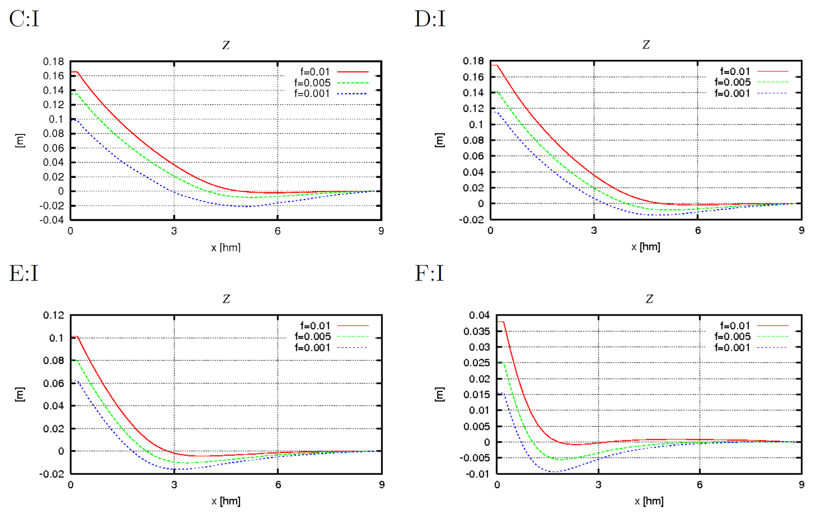
In a coastal zone characterized by a flat bottom with a constant slope and longitudinal homogeneity, the values of the averaged free surface elevation Z obtained from calculations should align with typical elevations associated with the presence of well-known phenomena such as set-up and set-down. Therefore, a primary significant test of the model was deemed to be the verification of calculation results conducted for bathymetric case I and various corresponding wave scenarios (C–F). Concurrently, a full range of bottom friction coefficient f values was employed in the calculations to assess its impact on the obtained values.The results of the calculations are illustrated in Figure 4.

For each wave scenario, based on the values of the averaged free surface elevation, it was possible to identify the location of the set-down zone (just before the wave breaking line) and the set-up zone (reaching its maximum near the shore). The value of set-down was close to zero with a bottom friction coefficient $f=0.01$ and increases as the value of this coefficient decreases. This pattern allows us to conclude that the obtained results are generally consistent with the classic findings of Longuet-Higgins [32], obtained under the assumption of no bottom friction, and with the results of other studies on this topic (see, for example, Hsu et al. [44]).

The Z values for scenarios C and D were similar, a consequence of the resemblance in wave height values for both cases. The strong dependency of the free surface elevation values on the function $H\left(x\right)$ was confirmed by the results obtained for wave scenarios E and F. In these instances, a reduction in Z values was observed, as well as a shift of the minimum values (set-down) toward the shore. Based on the calculations performed, no distinct influence of the wave approach direction to the shore on the values of free surface elevation was detected.

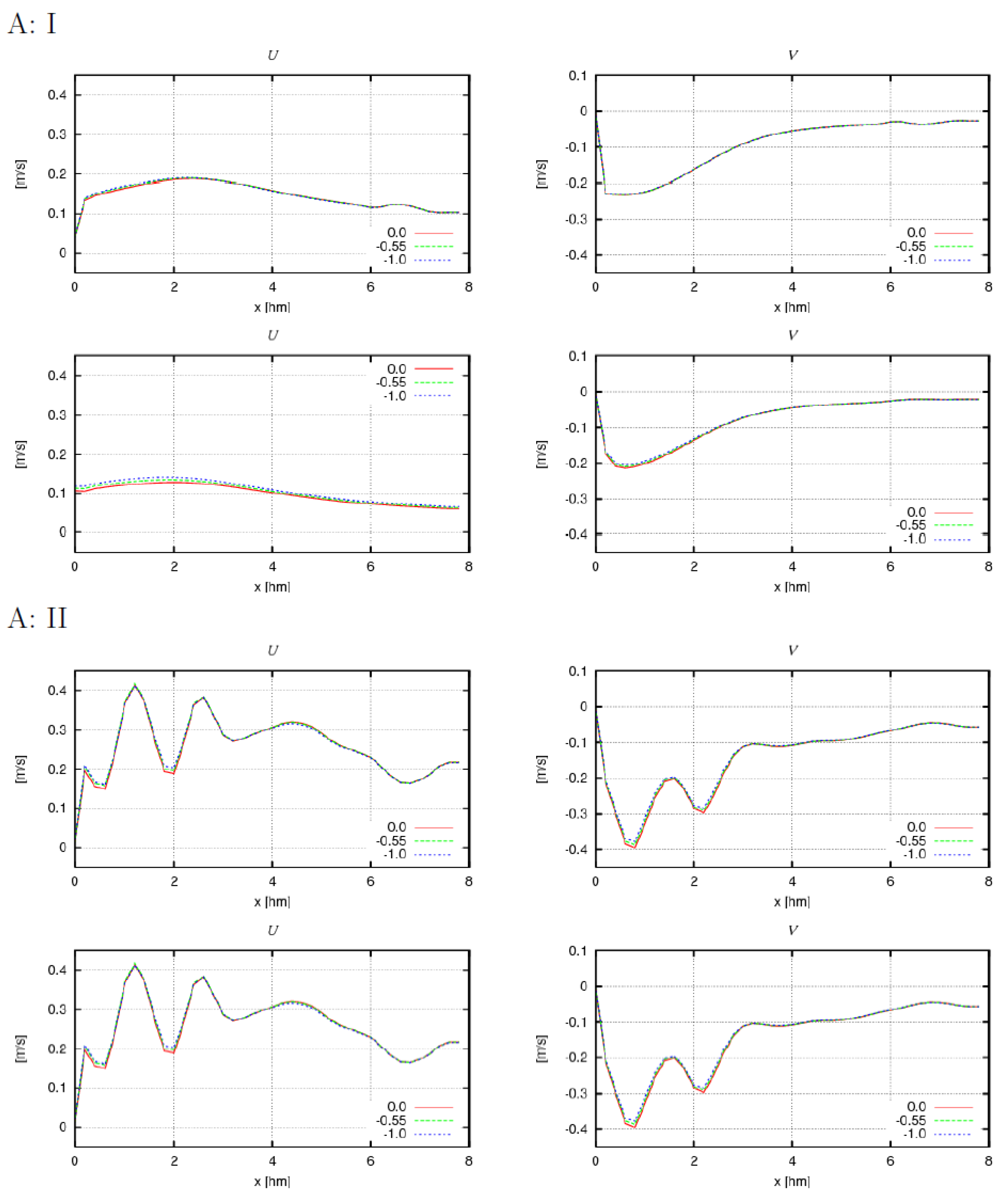
To determine the impact of the cross-shore bathymetric variability on velocity values, the results obtained for coastal zones I–II and wave data A and B are summarized below. The presented results, for both wave data A and B, were achieved using $f=0.01$. Given the certain similarities between wave fields A and B and the assignment of identical coefficient values (considering their significant impact on the outcomes), similar values for all presented magnitudes were obtained. The only observation worth noting is that the values obtained for case B are slightly higher. This is likely related to the less oblique wave approach to the shore.

The obtained values of free surface elevation (for conditions A and B) are consistent with the theoretical values and those measured under natural conditions (Figure 5).

Based on the results concerning flow velocity values for conditions A and B, it can be observed that they exhibit minimal vertical variability (see Figure 6 and Figure 7). This can be attributed to the specified value of the vertical turbulent viscosity coefficient and is fairly consistent with the velocity distributions measured in the coastal zone. In coastal zones I and II, the velocities U are positive while those for V are negative, which for one, relates to the assumed longitudinal homogeneity and for another, to the wave approach direction to the shore. Furthermore, the values obtained for these cases (I and II) based on calculations A and B do not significantly differ. From this, it may be inferred that the analytical solution for specific conditions can be successfully applied in areas with isobaths parallel to the shore.

5. Summary and Conclusions

A three-dimensional model of wave-induced currents was developed from the following equations:

$$\mathsf{\nabla }·\mathit{U}+{\partial }_{z}W=0,$$

(99a)

$${\partial }_t\mathit{U}+{\rho }^{-1}\mathsf{\nabla }·\mathit{R}=-g\mathsf{\nabla }Z+\mathsf{\Gamma }·\mathit{U},$$

(99b)

They were also developed from the following boundary conditions:

$$\begin{array}{ccc}\hfill W={\partial }_{t}Z,& \hfill & \hfill z=Z,\end{array}$$

(100a)

$$\begin{array}{ccc}\hfill W=-\mathit{U}·\mathsf{\nabla }D,& \hfill & \hfill z=-D,\end{array}$$

(100b)

$$\begin{array}{ccc}\hfill {\mathsf{\tau }}_b={\left.\left(\rho {\nu }_v{\partial }_z\mathit{U}\right)\right|}_{-D}=f\left({\mathit{U}}_b\right),& \hfill & \hfill z=-D,\end{array}$$

(100c)

$$\begin{array}{ccc}\hfill {\mathsf{\tau }}_s={\left.\left(\rho {\nu }_v{\partial }_z\mathit{U}\right)\right|}^0=-\frac{1}{2}\mathsf{\nabla }E,& \hfill & \hfill z=Z,\end{array}$$

(100d)

$$\begin{array}{c}\hfill {\partial }_{t}Z+\mathsf{\nabla }·\left(\mathit{Q}+\mathit{q}\right)=0,\mathrm{where}:\mathit{Q}=\underset{-D}{\overset{0^{-}}{\int }}\mathit{U}dz,\mathit{q}={\mathit{k}}^0{\left(\rho c\right)}^{-1}E,\end{array}$$

(100e)

$$\begin{array}{c}\hfill \rho {\partial }_t\left(\mathit{Q}+\mathit{q}\right)+\mathsf{\nabla }·\mathbf{S}=-\rho gD\mathsf{\nabla }Z+\rho \mathbf{G}·\mathit{Q}-{\mathsf{\tau }}_b.\end{array}$$

(100f)

The results obtained in this work are expected to be of importance for studies on ocean dynamics. They are particularly applicable to the hydrodynamics of wave-dominated coastal zones.

The major novel aspects elucidated by the study can be summarized as follows:

• Some new basic simplification rules appropriate for the problem considered were proposed;
• A new simplified relationship (tailored to the nature of the coastal zone) that describes the turbulent stress tensor was formulated and applied to equations describing wave–current interactions;
• Local (quasi-turbulent) wave-induced stresses were identified and treated as components of the three-dimensional radiation stress tensor;
• The distribution of the wave-induced momentum transport (radiation stress) as a function of the depth-independent variable was described;
• The presence of the virtual wave-induced stresses (the distributional part of the radiation stress tensor) at the averaged free surface was identified, and the stresses were quantified;
• A fully three-dimensional model describing the coastal zone hydrodynamics was developed;
• An approximate analytical solution for the special case of a coastal zone homogeneous in the longshore direction (with isobaths parallel to the shoreline) was proposed;
• An approximate analytical solution for the general case was proposed.

Further research should focus on the development of a numerical model that solves the equations presented.

References

- Longuet-Higgins, M.S. Longshore currents generated by obliquely incident sea waves: 1. J. Geophys. Res. 1970, 75, 6778–6789. [Google Scholar] [CrossRef]
- Longuet-Higgins, M.S. Longshore currents generated by obliquely incident sea waves: 2. J. Geophys. Res. 1970, 75, 6790–6801. [Google Scholar] [CrossRef]
- Dyhr-Nielsen, M.; Sorensen, T. Some sand transport phenomena on coast with bars. In Proceedings of the 12th International Conference on Coastal Engineering, ASCE, Washington, DC, USA, 13–18 September 1970; Volume 2, pp. 855–865. [Google Scholar]
- De Vriend, H.J.; Stive, M.J.F. Quasi-3d modelling of nearshore currents. Coast. Eng. 1987, 11, 565–601. [Google Scholar] [CrossRef]
- Sánchez-Arcilla, A.; Collado, F.; Lemos, M.; Rivero, F. Another quasi-3d model for surf-zone flows. In Proceedings of the 22th International Conference on Coastal Engineering, ASCE, Delft, The Netherlands, 2–6 July 1990; Volume 1, pp. 316–329. [Google Scholar]
- Garcez-Faria, A.F.; Thornton, E.B.; Stanton, T. A quasi-3d model of longshore currents. In Proceedings of the International Conference of Coastal Research in Terms of Large Scale Experiments (Coastal Dynamics ’95), ASCE, Gdansk, Poland, 4–8 September 1995; Volume 1, pp. 389–400. [Google Scholar]
- Nobuoka, H.; Mimura, N.; Kato, H. Three-dimensional nearshore currents model based on vertical distribution of radiation stress. In Proceedings of the 26th International Conference on Coastal Engineering, ASCE, Copenhagen, Denmark, 22–26 June 1998; Volume 1, pp. 829–842. [Google Scholar]
- Mellor, G.L. The three-dimensional current and surface wave equations. J. Phys. Oceanogr. 2003, 33, 1978–1989. [Google Scholar] [CrossRef]
- Mellor, G.L. Some consequences of the three-dimensional currents and surface wave equations. J. Phys. Oceanogr. 2005, 35, 2291–2298. [Google Scholar] [CrossRef]
- Mellor, G.L. The depth-dependent current and wave interaction equations: A revision. Phys. Oceanogr. 2008, 38, 2587–2596. [Google Scholar] [CrossRef]
- Kumar, N.; Voulgaris, G.; Warner, J.C. Implementation and modification of a three-dimensional radiation stress formulation for surf zone and rip-current applications. Coast. Eng. 2011, 58, 1097–1117. [Google Scholar] [CrossRef]
- Chou, Y.-J.; Holleman, R.C.; Fringer, O.B.; Stacey, M.T.; Monismith, S.G.; Koseff, J.R. Three-dimensional wave-coupled hydrodynamics modeling in South San Francisco Bay. Comput. Geosci. 2015, 85, 10–21. [Google Scholar] [CrossRef]
- Ranasinghe, R.S. Modelling of waves and wave-induced currents in the vicinity of submerged structures under regular waves using nonlinear wave-current models. Ocean Eng. 2022, 247, 110707. [Google Scholar] [CrossRef]
- Tang, S.; Yang, Y.; Zhu, L. Directing Shallow-Water Waves Using Fixed Varying Bathymetry Designed by Recurrent Neural Networks. Water 2023, 15, 2414. [Google Scholar] [CrossRef]
- Xia, H.; Xia, Z.; Zhu, L. Vertical variation in radiation stress and wave-induced current. Coast. Eng. 2004, 51, 309–321. [Google Scholar] [CrossRef]
- Kołodko, J.; Gic-Grusza, G. A note on the vertical distribution of momentum transport in water waves. Oceanol. Hydrobiol. Stud. 2015, 44, 563–568. [Google Scholar] [CrossRef]
- Chybicki, W. On Vertical Variations of Wave-Induced Radiation Stress Tensor. Arch. Hydro-Eng. Environ. Mech. 2008, 55, 83–93. [Google Scholar]
- Dolata, L.F.; Rosenthal, W. Wave setup and wave-induced currents in coastal zones. J. Geophys. Res. 1984, 89, 1973–1982. [Google Scholar] [CrossRef]
- Mellor, G.L. On theories dealing with the interaction of surface waves and ocean circulation. J. Geophys. Res. Oceans 2016, 121, 4474–4486. [Google Scholar] [CrossRef]
- Mellor, G.L. A combined derivation of the integrated and vertically-resolved, coupled wave-current equations. J. Phys. Oceanogr. 2015, 45, 1453–1463. [Google Scholar] [CrossRef]
- McWilliams, J.C.; Restrepo, J.M. The wave-driven ocean circulation. J. Phys. Oceanogr. 1999, 29, 2523–2540. [Google Scholar] [CrossRef]
- Mellor, G.L. On Surf Zone Fluid Dynamics. J. Phys. Oceanogr. 2021, 51, 37–46. [Google Scholar] [CrossRef]
- Svendsen, I.A.; Lorenz, R.S. Velocities in combined undertow and longshore currents. Coast. Eng. 1989, 13, 55–79. [Google Scholar] [CrossRef]
- Nobuoka, H.; Mimura, N. 3-D nearshore current model focusing on the effect of sloping bottom on radiation stresse. In Proceedings of the 28th International Conference on Coastal Engineering, ASCE, Cardiff, UK, 7–12 July 2002; Volume 1, pp. 836–848. [Google Scholar]
- Lee, J.L.; Wang, H. A quasi-3D surf zone model. In Proceedings of the 24th Conference on Coastal Engineering, Kobe, Japan, 23–28 October 1994; Volume 2, pp. 2267–2281. [Google Scholar]
- Smith, J.A. Wave-current interactions in finite depth. J. Phys. Oceanogr. 2006, 36, 1403–1419. [Google Scholar] [CrossRef]
- Cieślikiewicz, W.; Gudmestad, O.T. Stochastic characteristics of orbital velocities of random water waves. J. Fluid Mech. 1993, 255, 275–299. [Google Scholar] [CrossRef]
- Svendsen, I.A.; Putrevu, U. Surf-zone hydrodynamics. In Advances in Coastal and Ocean Engineering; Liu, P.L., Ed.; World Scientific: Singapore, 1996; pp. 1–78. [Google Scholar]
- Rivero, F.J.; Arcilla, A.S. On the vertical distribution of huwi. Coast. Eng. 1995, 25, 137–152. [Google Scholar] [CrossRef]
- Mocke, G. Structure and modeling of surf zone turbulence due to wave breaking. J. Geophys. Res. 2001, 106, 17039–17058. [Google Scholar] [CrossRef]
- Bradford, S.F. Numerical simulation of surf zone dynamics. J. Waterw. Port Coast. Ocean Eng. 2000, 126, 1–13. [Google Scholar] [CrossRef]
- Longuet-Higgins, M.S.; Stewart, R.W. Radiation stress in water waves; a physical discussion with applications. Deep-Sea Res. 1964, 11, 529–562. [Google Scholar]
- Stive, M.J.F.; Wind, H.G. A study of radiation stress and set-up in the nearshore region. Coast. Eng. 1982, 6, 1–25. [Google Scholar] [CrossRef]
- Stive, M.J.F.; Wind, H.G. Cross-shore mean flow in the surf zone. Coast. Eng. 1988, 19, 325–340. [Google Scholar] [CrossRef]
- Shi, F.; Svendsen, I.A.; Kirby, J.T.; Smith, J.K. A curvilinear version of a quasi-3d nearshore circulation model. Coast. Eng. 2003, 49, 99–124. [Google Scholar] [CrossRef]
- Battjes, J.A.; Sobey, R.J.; Stive, M.J.F. Nearshore circulation. In The Sea: Ocean Engineering Science, 9; Le Mehaute, B., Hanes, D.M., Eds.; John Wiley & Sons: Hoboken, NJ, USA, 1990; pp. 468–493. [Google Scholar]
- Elsner, J.W. Turbulencja Przepływów; Państwowe Wydawnictwo Naukowe PWN: Warszawa, Poland, 1987. (In Polish) [Google Scholar]
- Longuet-Higgins, M.S.; Stewart, R.W. Radiation stress and mass transport in gravity waves with application to “surf beats”. J. Fluid Mech. 1962, 13, 481–504. [Google Scholar] [CrossRef]
- Kinsman, B. Wind Waves: Their Generation and Propagation on the Ocean Surface; Prentice-Hall, Inc.: Upper Saddle River, NJ, USA, 1965. [Google Scholar]
- Crapper, G.D. Introduction to Water Waves; Elis Horwood Limited: Chichester, UK, 1984. [Google Scholar]
- Philips, O.M. The Dynamics of the Upper Ocean; Cambridge University Press: Cambridge, UK, 1977. [Google Scholar]
- Dudkowska, A.; Boruń, A.; Malicki, J.; Schönhofer, J.; Gic-Grusza, G. Rip currents in the non-tidal surf zone withsandbars: Numerical analysis versus field measurements. Oceanologia 2020, 62, 291–308. [Google Scholar] [CrossRef]
- Booij, N.; Holthuijsen, L.H.; Ris, R.C. A third-generation wave modelfor coastal regions. J. Geophys. Res. 1999, 104, 7649–7666. [Google Scholar] [CrossRef]
- Hsu, T.-H.; Hsu, J.R.-C.; Weng, W.-K.; Wang, S.-K.; Ou, S.-H. Wave setup and setdown generated by obliquely incident waves. Coast. Eng. 2006, 53, 865–877. [Google Scholar] [CrossRef]
Figure 1.
Visual representation of the three-dimensional mean velocity distribution in the coastal zone.
Figure 2.
Visual representation of the vertical distribution of the force generating the horizontal momentum transport.
Figure 3.
The current model input data: water depth. I—flat-bottom, constant-slope profile; II—multibar profile with isobaths parallel to the shoreline.
Figure 4.
Mean free surface elevation Z obtained from a general solution for wave parameters C–F and bathymetric data I. Calculations were performed for different values of bottom friction coefficient f.
Figure 5.
Mean free surface elevation Z obtained from a general solution for wave parameters A–B and bathymetric data I–II. Calculations were performed for different values of bottom friction coefficient f.
Figure 6.
Current velocity U (left) and V (right) for different values of (depth levels) obtained from calculations based on the general solution (upper figure) and the special solution (lower figure) corresponding to the wave parameters A and the bathymetric data I–II.
Figure 7.
Current velocity U (left) and V (right) for different values of (depth levels) obtained from calculations based on the general solution (upper figure) and the special solution (lower figure) corresponding to the wave parameters B and the bathymetric data I–II.