Life Cycle Assessment Methodology Applied to a Wastewater Treatment Plant

Abstract

Wastewater treatment plants are highly energy-intensive systems. This research uses Life Cycle Assessment (LCA) to determine the impacts generated during the operation of a wastewater treatment plant. Three different scenarios are analyzed: a baseline scenario that considers a conventional activated sludge treatment technology exploiting data from an existing plant located in central Italy, a second scenario that involves the implementation of MBR technology applied to the baseline scenario, and finally a third scenario that consists of the addition of an anaerobic digester that allows energy recovery from biogas production, followed by a photovoltaic plant capable of supplying the plant energy demand. Global warming potential, eutrophication, and acidification are the environmental categories considered most relevant to emissions. The results showed that the effluent had the highest impact in terms of CO₂ equivalent in all three situations due to the presence of N₂O. Since emissions from biological processes, transportation, and wastewater are almost similar in all three scenarios, it is preferable to focus on the environmental impacts associated with energy consumption. The third scenario involves careful resource management and the use of treatment technologies that allow for a reduction in the use of nonrenewable energy sources in favor of renewable ones.

1. Introduction

In a historical period such as the one we are living through nowadays, in which the consequences of industrial development, population growth, and more generally anthropization are increasingly evident and concerns about environmental sustainability are now an integral part of everyday life, it is necessary to implement environmental protection measures. Indeed, the economic, political, and industrial landscape is shifting towards the accomplishment of the principle of sustainable development, i.e., development that meets the needs of current generations without compromising the freedom of future generations to meet their own [1]. Therefore, efforts are being made to implement tools that are in line with energy–environmental sustainability.

Wastewater treatment plants can play an important role within this pathway, as they are energy-intensive systems, thus leading to significant environmental impacts [2]. Suffice it to say that about 4% of global energy is used to treat, pump, and distribute water [3]. It is necessary to improve the efficiency of these plants in order to get closer to the “zero pollution” concepts proposed in the European Green Deal set for 2050, as well as to comply with the Kyoto Protocol limits on emissions [4].

The Life Cycle Assessment procedure (LCA) is one of the analytical tools often used to define the complex relationship between production systems and the environment, and it is employed here to evaluate environmental assessment. This methodology enables the determination of emissions generated throughout the life cycle of a product or process, “from cradle to grave” allowing comparisons between scenarios and estimating which one has the lowest impacts [5].

Several studies have applied the LCA methodology to wastewater treatment plants to assess their impacts [6,7,8,9]. Allami et al. [10] used the LCA methodology to define the best plant configuration among three different scenarios: a traditional activated sludge plant with a sand filter, another with the use of a sand filter and nitrogen removal, and finally a plant with the implementation of MBR technology. The analysis showed that the configuration with MBR used less energy and consequently produced lower emissions than the other two configurations using sand filters. It is therefore important to define the flow pattern of the plant. Although the MBR is considered a highly energy-intensive system, it consumes less energy than sand filters.

A further configuration considers the use of an anaerobic digester, where the application of biogas instead of natural gas can reduce the negative impacts of fossil fuels by approximately three times. The result was studied by Tabesh et al. [11] through the application of the LCA methodology, which was able to provide an environmental impact analysis and simplify decision making in the wastewater treatment sector.

Also, Pasqualino et al. [12] used LCA to compare different plant solutions, reaching the conclusion that the implementation of the anaerobic digester can provide sufficient energy to power all the plant stages, thus reducing the environmental impact.

In the study by Zhang et al. [13], LCA methodology was used to determine the benefit of reusing tertiary effluent for industrial and domestic purposes, resulting in water savings. This type of benefit is considered equivalent to energy savings that would otherwise be used to produce the same amount of tap water. According to Zhang et al. [13], the average energy consumption for tap water production in the city of Xi’an is around 4440 kJ/m³, considering both the development of water resources and the application of water treatment.

Another case study in China was analyzed by Li et al. [14], where LCA was used to evaluate the environmental impacts in different phases of WWTP: construction, operation, sludge landfilling, and transportation of chemicals to the plant. Based on the study, the Kunshan wastewater treatment plant’s environmental impacts are mainly due to the operation and maintenance phases. In fact, under the hypothesis of 50 years of operation of the plant and of electricity production exclusively from a coal-fired power plant, the consumption of electricity by the plant provides the most significant contribution to the depletion of abiotic resources (91%), global warming (94.9%), photochemical oxidation (88.8%), and acidification (78.9%).

Amores et al. [15] compared three scenarios using LCA to perform an analysis of the different phases (water abstraction, drinking water treatment, intermediate pumping, distribution network, wastewater collection, and wastewater treatment) of the urban water cycle in Terragona, Spain: (1) current situation, (2) use of reclaimed water and desalination plants, and (3) reclaimed water to provide water during droughts. In all three scenarios, the main source of impact was the energy consumed through the collection and intermediate pumping of fresh water.

The following article presents the use of LCA methodology during the operational phases of a wastewater treatment plant. Data from an existing plant in central Italy were used as input for the study. Through the application of the LCA, it was possible to compare the base case of a conventional activated sludge plant with two different scenarios, which are part of the development strategy of the plant management, to be able to compare the impacts generated. The application of LCA to different scenarios and its environmental results depend on several boundaries. The reference scenario (scenario A), a typical sludge-activated treatment, will be compared to a second scenario where the MBR technology was added (scenario B), and to a third scenario where the implementation of scenario A is the introduction of the anaerobic digester in the sludge line with energy recovery together with a photovoltaic plant in order to satisfy the energy demand of the plant (scenario C) are used. No commercial software was used in this study, but a specific one was designed to best represent the study needs. According to the analysis of the three scenarios, the environmental categories of acidification and eutrophication remain unchanged because they are related to transportation, and the latter does not alter depending on the plant configuration used. The situation is different for the global warming potential, where there are significant differences according to energy consumption. The third scenario, in fact, which envisages the adoption of the anaerobic digester to partially feed the plant, has very low emissions, unlike the second scenario, which, using MBR technology, has considerable impacts, the greatest among the three scenarios analyzed.

2. Materials and Methods

The present study uses LCA to quantitatively determine the environmental input and output flows of energy and matter throughout the life of a WWTP. This methodology differs from environmental impact assessment (EIA) since the latter is based on actual impacts, quantified considering the alterations introduced into the environmental system, while the LCA study is based on the concept of potential impact. Through this tool, it is determined whether, under certain conditions, any emission or extraction can be transformed into a contribution to different impact categories [16].

Life Cycle Assessment has several applications and makes it possible to compare products with the same function, compare the environmental impact of a product with a referenced standard, identify the process that results in the greatest environmental impact over the life cycle of a system or a product, design new production processes or new products in general, and evaluate different scenario comparisons and thus, is a planning support tool for decision-makers or stakeholders [2].

According to ISO 14040:1997 [17] (International Standard Organisation, 1997) and ISO 14044:2006 [18] (International Standard Organisation, 2006), LCA is a procedure consisting of four main steps:

• Goal and scope phase, composed of the definition of the system boundaries and scope system functions, functional units, allocation procedures, impact types, required data, assumptions or simplifications, and finally, the quality of the data [19];
• Inventory analysis, known as Life Cycle Inventory (LCI) in which the data needed for the study system are reported [19]. In this phase, for example, the quantities of raw material requirements or energy sources associated with each stage of the life cycle of a product or process are reported [20];
• Impact assessment phase, defined as Life Cycle Impact Assessment (LCIA): Once the data have been collected, they must then be converted into impact measures to assess the environmental effects of the system under consideration [21]. After the equivalence factors definition, the final result will be environmental profiles consisting of a series of impact scores for each category [16]. The different existing impact categories include global warming, ozone depletion, human toxicity, ecotoxicity, photo-oxidation, acidification, eutrophication, odors, noise, radiation, accidents, and disasters. Several authors discuss the above impact categories, assessing what the emissions are for each category, excluding odors, noise, radiation, accidents, and ecotoxicity [21,22]. Further studies have found that energy consumption is one of the most impactful factors within sewage treatment plants [23,24,25,26]. Furthermore, some literature studies [11,14,27,28,29,30] analyze, starting from impact categories, different environmental effects at different stages of construction, operation, and demolition;
• Data interpretation, defined by ISO 14044 [18], with the aim of performing a critical evaluation of the entire LCA study.

2.1. Goal and Scope Definition

The goal of this model is to demonstrate how LCA can be used as a tool for technological or management choices by comparing the impacts generated by two or more different configurations of wastewater treatment plants. In the reported case study, a traditional activated sludge plant is used to represent the first scenario under analysis, while the second scenario considers the implementation of MBR (Membrane BioReactor) technology removing the secondary settler in order to have better performance in effluent clarification. Finally, a third scenario considers the implementation of an anaerobic digester within the traditional wastewater treatment plant. This system uses biogas energy to partially power the plant, while a photovoltaic system provides the remaining energy required to create a self-sufficient plant.

2.2. Life Cycle Impact Assessment (LCIA)

The reported study considers the following impact categories as the most affected by sewage treatment plants: global warming potential (GWP), potential acidification (PA), and potential eutrophication (PE). Within each impact category, an equivalence factor is defined to express the potential environmental impact of the considered substance relative to a weight unit of the reference substance. The conversion factors given in the following paragraphs were extrapolated from the Ecoinvent database, within which the CML (Centrum voor Milieukunde, Leiden, The Netherlands) 2001 software was used as a reference. Once the equivalence factors have been defined for each environmental sector, the impact is calculated as the product between the output produced in terms of emissions and the related conversion factor.

2.3. Functional Unit (F.U.)

The functional unit is a measurable and clearly determined quantity (ISO 14040:2006), which is essential for comparing different scenarios. In this study, 1 m³/d of influent was used as a functional unit, since it has been considered in several studies with satisfactory results [22,27,31].

2.4. System Boundaries

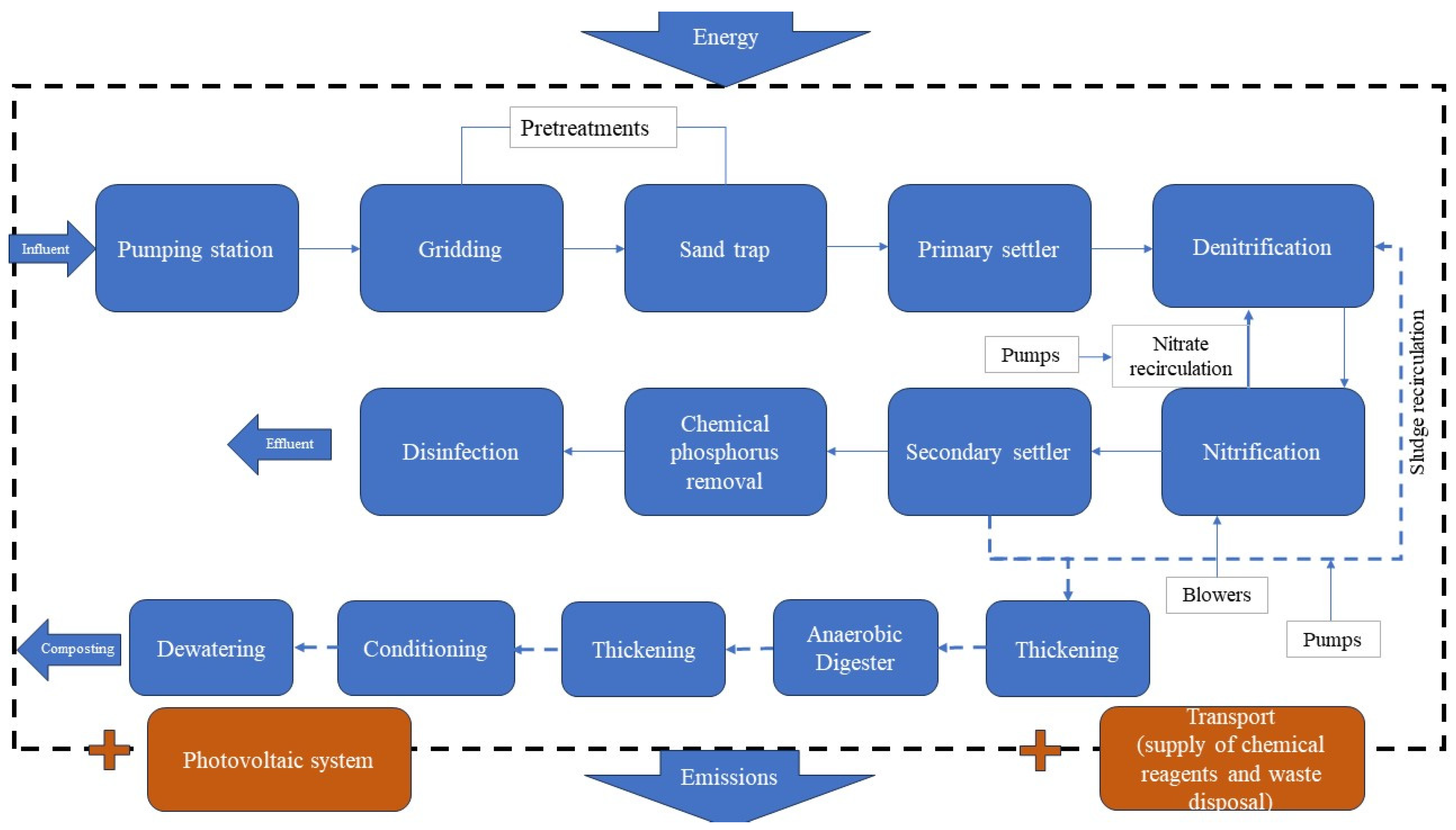
The system boundaries for the three case studies are shown in Figure 1, Figure 2 and Figure 3. Within the system, the incoming energy flows necessary for the operation of the electromechanical components of the various sections, the transport of materials into and out of the plant, and finally the pollutant emissions produced from these processes are considered. The treatment of solid sludge leaving the plant as well as the treatment of further different wastes from the various sections of the plant do not fall within the boundaries of the system. The cradle-to-gate approach is then just for the main stream of wastewater. Sludge is briefly considered in the paper just for a rough evaluation of the different possible systems of disposal in terms of GWP impacts. The flow diagram of scenario A with its system boundaries is shown in Figure 1.

One of the most advanced technologies that can be used in wastewater treatment plants is bioreactive membranes (MBRs), which have been largely studied [11,16,21,27,31,32,33,34,35]. MBR allows the enhancement of effluent quality.

The MBR system makes use of a side stream ultrafiltration module. Some components, such as the secondary settler tank, are eliminated if compared to the traditional activated sludge case. Flow diagram of scenario B is shown in Figure 2.

In the third scenario, the conventional activated sludge process is combined with an anaerobic digester, allowing greater sludge stabilization if compared with scenario A, reducing the mass of solid organic material and pathogens in the sludge itself [36]. The most important aspect is that the anaerobic process produces biogas with characteristics suitable to be used as a biofuel to generate energy [37]. In this scenario, a photovoltaic system was also added to try to satisfy the plant’s remaining energy requirements, which the digester cannot supply. Flow diagram of scenario C is shown in Figure 3.

2.5. Life Cycle Inventory (LCI)

The primary data used in the LCA application were collected from a wastewater treatment plant in central Italy (

Table 1. Input data from wastewater treatment plant located in central Italy.

Parameters	Symbol	Value	Unit of Measurement
Number of inhabitant equivalent	P	75,000	Inhab. equivalent
Per capita net water supply	D	400	L/inhab*d
Sewer inflow coefficient	Φ	0.8	adim
Average flow rate	QA	24,000	m3/d

,

Table 2. Concentrations of incoming pollutants.

Parameters	Value	Unit of Measurement
Influent concentration BOD5	104	g/m3
Influent concentration COD	397	g/m3
Influent concentration TSS	284	g/m3
Influent concentration TKN	37	g/m3
Influent concentration PTOT	10	g/m3

and

Table 3. Concentrations of pollutants in the effluent.

Parameters	Value	Unit of Measurement
Effluent concentration BOD5	25	g/m3
Effluent concentration COD	62	g/m3
Effluent concentration TSS	2	g/m3
Effluent concentration TKN	1.45	g/m3
Effluent concentration PTOT	0.8	g/m3

).

The study was carried out by subdividing the plant according to the different occurring treatment phases. For each phase, the energy associated with the operation of the single section was calculated using the technical specification of the electromechanical components present:

Energy [kWh/d] = P [kW/d] * t [h] * n [adimensional]

(1)

where P is the machinery power, t represents the hours of machinery work, and finally n is the number of machineries used. Once the total required energy is defined, the associated CO₂ emission is determined using the emission factor EF_EP referred to the national energy production equal to 380 gCO₂/kWh (Ecoinvent v 3.8):

CO₂ [g/d] = Energy [kWh/d] * EF_EP [gCO₂/kWh]

(2)

In biological processes, direct CO₂ emissions should be considered due to the bacteria methabolism: during bacterial growth, in fact, chemical reactions are responsible for the production of CO₂, which can be evaluated stoichiometrically:

C₅H₇O₂N + 5O₂ → 5CO₂ + 2H₂O + NH₃

(3)

EF [gCO₂/gSSV] = [(44 * 5) gCO₂/mol]/[113 gSSV/mol] = 1.947 gCO₂/gSSV

(4)

where EF is the conversion factor defined through the carbon dioxide molecular weight multiplied by the number of moles and divided for the organic substance molecular weight. By means of the conversion factor determined stoichiometrically, the CO₂ associated with biological processes is defined as follows:

CO₂ [g/d] = EF [gCO₂/gSSV] * Q_A [m³/d] * (COD_I[g/m³]-COD_E[g/m³])

(5)

In which Q is the average flow rate (Table 1) and COD_I and COD_E are, respectively, the influent concentration and the effluent concentration of COD (Table 2 and Table 3).

IPCC guidelines [38] and several authors [39] consider that the biogenic production of CO₂ should not be included in the amounts of GWP, and some chemicals, like fossil carbon-based substances, should be included within a range between 4–14%. In the present study, 9% of the biogenic CO₂ production was taken into account. N₂O is also produced in the plant for the protein content present in wastewater flow. Due to its high greenhouse potential, which is 298 times greater than that of CO₂, it has a significant impact on the environment.

The direct N₂O emissions is calculated as follows according to IPCC Chapter 6 [40], whose terms are defined in

Table 4. Parameters of Equation (6) and their typical values for direct N₂O emissions [41].

Parameters	Symbol	Default	Range	Unit of Measurement
Number of inhabitant equivalent	P	Specific	Specific	Inhab
Utilization factor of the plant	U	Specific	Specific	Adimensional
Industrial and commercial protein production factor	FIND-COM	1.25	1–1.5	Adimensional
Emission factor (from IPCC)	EFplant	3.2	2–8	g N2O/inhab*year

:

N₂O [kg/year] = P * U * F_IND-COM * EF_plant

(6)

About the utilization factor, it is equal to one in case the plant is in operation all year round, such as in this study. In addition to direct production, there is also indirect N₂O emission in the effluent [40]:

N₂O_Eff [kg/year] = N_Eff * EF_Eff * (44/28)

(7)

where N_Eff is the nitrogen output load, EF_Eff is the N₂O emission factor for outlet flow, and the factor (44/28) is a conversion from kg of N₂O-N to kg of N₂O. The nitrogen output load is calculated as follows [41], whose terms are defined in

Table 5. Parameters of Equation (8) and their typical values for indirect N₂O emissions.

Parameters	Simbol	Default	Range	Unit of Measurement
Number of inhabitant equivalent	P	Specific	Specific	inhab
Per capita protein consumption	Protein	Specific	Specific	kg_proteins/inhab*year
Protein production factor	FIND-COM	1.25	1–1.5	Adimensional
Protein consumption factor	FNON-COM	1.3	1–1.5	Adimensional
Emission factor for outlet flow	EFEff	0.005	0.0005–0.25	kgN2O/kgN
Nitrogen fraction in proteins	FNPR	0.16	0.15–0.17	kgN/kg_Proteins
Nitrogen removed with sludge	NR	13.4% of TKN in input		kg/year

:

N_Eff [kg/year] = (P * Protein * F_NPR * F_NON-COM * F_IND-COM) − N_R

(8)

Once the amount of N₂O produced has been calculated and transformed in g/d, it is then converted to CO₂ via the equivalence factor (Ecoinvent CML, 2001).

3. Results and Discussion

3.1. Scenario A

Table 6. Energy consumption [kWh/d per F.U.] related to the number of electromechanical components in the different sections of the plant—scenario A.

Sections	Number of Electromechanical Components	kWh/d Per F.U.
Pumping station	1	0.055
Pretreatments	8	0.026
Primary settler	2	0.0045
Biological	7	0.21
Secondary settler	3	0.0028
Chemical phosphorus removal	2	0.0019
Disinfection	2	0.0010
Thickening	4	0.0012
Conditioning	6	0.0037
Dewatering	1	0.019
Total	34	0.33

and the related Figure 4 show the total energy of the various sections according to the electromechanical components present (the total kWh/d is referred to as the functional unit):

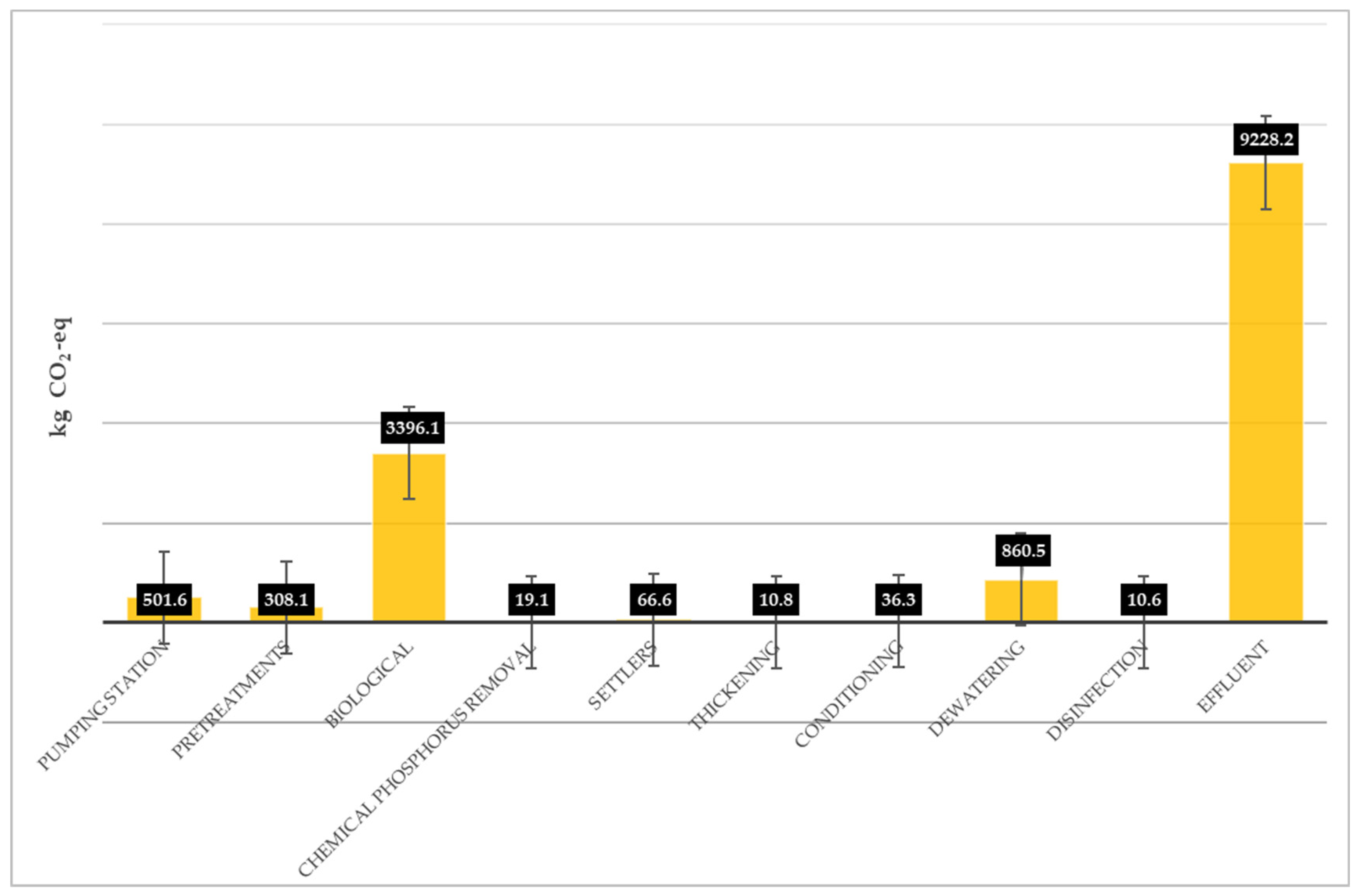
Once the required energy for each section of the plant has been defined, the related CO₂ emissions are determined through Equation (2) and reported in

Table 7. CO₂ emissions [kg/d per F.U.] due to energy consumption, transportation, and direct emissions—scenario A.

Sections	kg/d Per F.U.
Pumping station	0.021
Pretreatments	0.013
Primary settler	0.0017
Biological	0.13
Chemical phosphorus removal	0.00080
Secondary settler	0.0011
Disinfection	0.00044
Thickening	0.00045
Conditioning	0.0015
Dewatering	0.035
Effluent	0.38
Total	0.591

and Figure 5.

The data reported in Table 7 and shown in Figure 5 demonstrate that the biological reactor contributes to 22% of the total CO₂ emissions for its energy consumption, and the largest contribution derives from the effluent with its N₂O content [42].

In addition to energy-related CO₂ emissions, the transport of waste materials to treatment or disposal, as well as the delivery of chemical supplies, all contribute to additional emissions that must be considered. The operating transports are reported in

Table 8. Transport emissions [g/d per F.U.] for chemical reagents and waste disposal.

Sections	NOX	CO	NH3	SO2	N2O	CO2	Unit of Measurement
Pretreatments	1.0 × 10−2	3.3 × 10−3	3.2 × 10−5	1.2 × 10−5	1.0 × 10−4	2.7 × 100	g/d per F.U.
Chemical phosphorus removal	2.6 × 10−4	8.5 × 10−5	8.3 × 10−7	3.1 × 10−7	3.4 × 10−6	7.1 × 10−2	g/d per F.U.
Disinfection	2.5 × 10−4	8.0 × 10−5	7.8 × 10−7	2.9 × 10−7	3.1 × 10−6	6.7 × 10−2	g/d per F.U.
Conditioning	3.9 × 10−4	1.2 × 10−4	1.2 × 10−6	4.6 × 10−7	4.9 × 10−6	1.0 × 10−1	g/d per F.U.
Dewatering	1.0 × 10−1	3.1 × 10−2	3.0 × 10−4	1.2 × 10−4	1.2 × 10−4	2.6 × 101	g/d per F.U.

.

Figure 6 shows which sectors of the plant have the greatest environmental impact in terms of GWP. The effluent greatly exceeds the values of the other sections due to the presence of N₂O. The biological reactor is surely one of the most impactful sections of the system, since it requires a large quantity of energy and, in addition to the energy required for operating, there is additional CO₂ production as a result of reactions by micro-organisms, which is assumed equal to 9% of the biogenic activity, as previously reported.

Within the potential acidification, pollutants such as NO_X, SO₂, and NH₃ emitted by vehicle exhausts are considered. Thus, acidification has impact contributions at the plant stages in which road transport is considered. It reaches a peak in the dewatering section and in the pretreatments due to the transportation to further treat or dispose of dewatered sludge and screenings, respectively. The values obtained in terms of kg SO₂ equivalent are 1.6 kg SO₂ equivalent/d for the dewatering section and 0.2 kg SO₂ equivalent/d for the screenings. They represent the contribution to the PA impact from the plant operating phase. The effluent has a very high eutrophication potential, caused by the release of residual phosphates eventually not removed during treatment. Regarding the PE impact, the effluent has the highest contribution equal to 67.1 kg PO₄ equivalent/d. This high value is linked to the presence of N₂O, which contributes to the PE impact. Smaller contributions are also present in the biological section (0.2 kg PO₄ equivalent/d) and dewatering (0.3 kg PO₄ equivalent/d). Both contributions are due to the residual phosphorus present in the wastewater mainstream and in the extracted sludges.

3.2. Scenario B

As mentioned above, the second scenario considers the implementation of MBR technology in the plant.

Table 9. Energy consumption [kWh/d per F.U.] related to the number of electromechanical components in the different sections of the plant—scenario B.

Sections	Number of Electromechanical Components	kWh/d Per F.U.
Pumping station	1	0.055
Pretreatments	8	0.026
Primary settler	2	0.0045
Biological	7	0.19
MBR	3	0.22
Chemical phosphorus removal	2	0.0019
Disinfection	2	0.0010
Thickening	4	0.0012
Conditioning	6	0.0037
Dewatering	1	0.019
Total	39	0.51

and the related graph in Figure 7 show the energy in kWh/d per functional unit associated with each compartment and based on the number of electromechanical components used.

The energy-related CO₂ emissions are determined through Equation (2).

Table 10. CO₂ emissions [kg/d per F.U.] due to energy consumption, transportation, and direct emissions—scenario B.

Sections	kg/d Per F.U.
Pumping station	0.021
Pretreatments	0.013
Primary settler	0.0017
Biological	0.12
MBR	0.08
Chemical phosphorus removal	0.00080
Disinfection	0.00044
Thickening	0.00045
Conditioning	0.0015
Dewatering	0.035
Effluent	0.38
Total	0.66

shows the carbon dioxide emissions related to energy consumption, transportation, and biological processes in scenario B. The same data are reported in Figure 8.

The results for transport impacts (PA, PE, and GWP) are the same as those reported for scenario A (Table 8), since the assumption is that the implementation of the MBR technology does not involve further material or larger waste transports.

The addition of MBR technology reduces the biological reactor’s energy consumption compared to scenario A (3396.1 kg CO₂ eq.—A → 31772.2 kg CO₂ eq.—B) due to the removal of some electromechanical components, such as the energy-intensive recirculation pumps. However, the traditional activated sludge plant requires more energy when the MBR is used in place of the secondary settler (Figure 9). Similarly to scenario A, the environmental category of GWP is also the most impactful, as well as the contribution of the effluent is larger than the other items due to the presence of the pollutant N₂O (Figure 9) [42].

3.3. Scenario C

In scenario C, an anaerobic digester is added to the sludge line. The anaerobic digestion process enables the biological stabilization of sewage sludge and the production of biogas, which is composed of CH₄ (60%) and CO₂ (40%), with traces of further substances (such as H₂S, N₂, and H₂). With regard to the treatment of secondary sludge, biogas production rate is around 28m³/(10³ inhab*d). Biogas has a wide range of applications, including the heating of the digesters themselves as well as the generation of mechanical energy and/or electricity. In

Table 11. Energy from biogas [kWh/d per F.U.].

Parameters	Value	Unit of Measurement
Biogas production per habitant	0.028	m3/inhab*d
Total biogas production	1400	m3/d
CH4 in biogas	60	%
Total CH4 production	840	m3/d
Conversion factor (CF)	10.7	kWh/m3
Energy from biogas	0.37	kWh/d per F.U.

are reported all the data necessary to calculate the energy obtained from biogas, and in

Table 12. Energy necessary for digester operation [kWh/d per F.U.].

Parameters	Value	Unit of Measurement
Dewatered sludge	5400	kg/d
Final sludge temperature	35	°C
Sludge inlet temperature	10	°C
Heat required for digester	157.5	J/d
Specific heat sludge	4200	J/(kg*°C)
Conversion factor	2.8 × 10−8	kWh/J
Energy required for digester operation	6.5 × 10−3	kWh/d per F.U.

is reported the energy required for the digestion operation, both in kWh/d per functional unit. Equations (9) and (10) show the formulas used to calculate, respectively, the energy obtained from the biogas and required to operate the digester:

Energy obtained from biogas [kWh/d per F.U.] = CH₄_production [m³/d] * CF [kWh/m³]

(9)

where the production of CH₄ and CF (conversion factor) are reported in Table 13. Regarding the calculation of methane production, this is calculated by taking 60% of the biogas production from the total number of inhabitants to be served.

An estimate of the amount of heat required to heat the sludge can be made using the following approach:

Q [J/d] = specific heat sludge [J/kg°C] * (Final sludge temperature [°C]—Sludge inlet temperature [°C]) * sludge quantity [kg/d]

(10)

The product between the heat required for the digester and the conversion factor in Table 12 gives the energy required for digester operation.

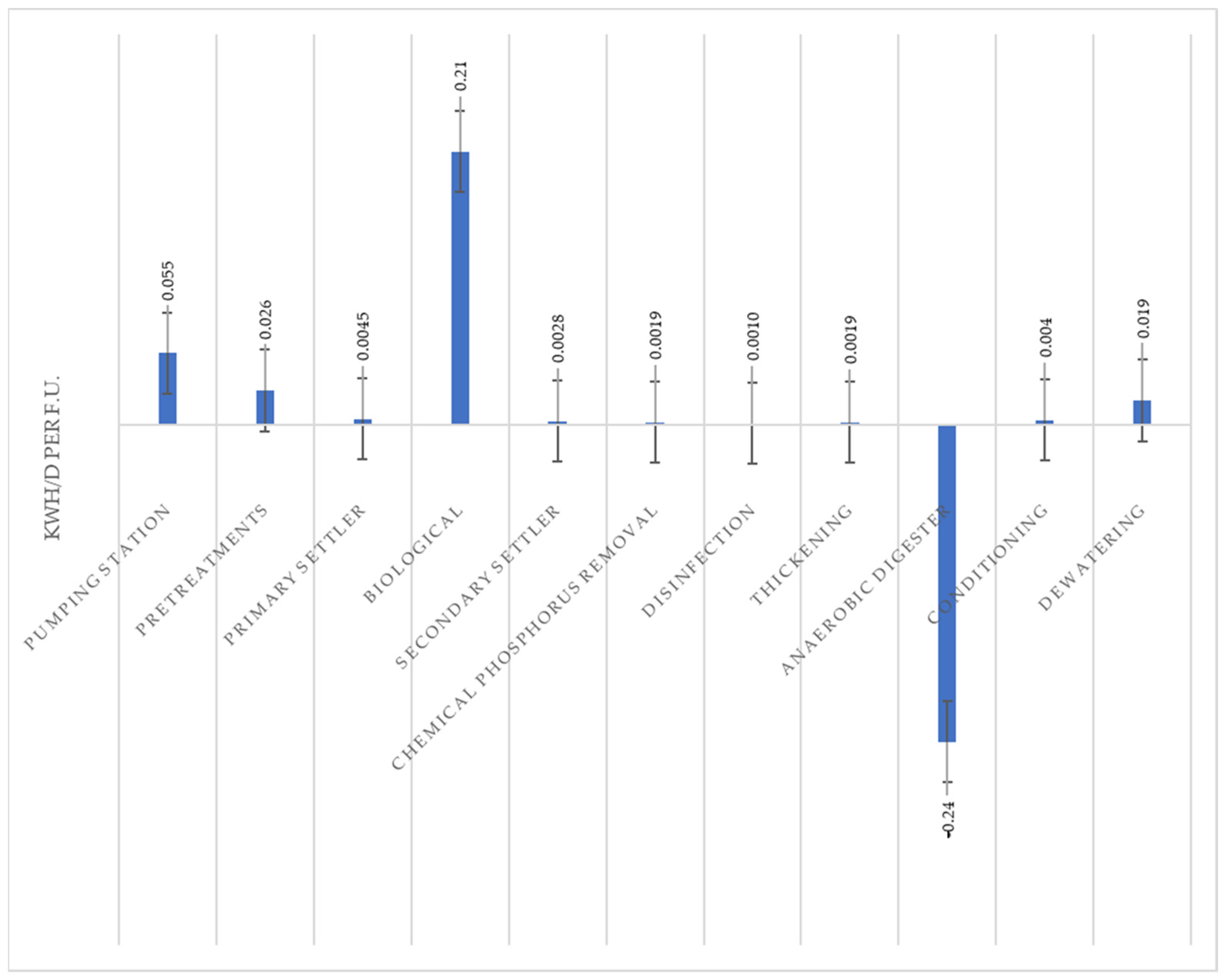
The energy used within the plant for each section is shown in Figure 10. The negative value in reference to the anaerobic digester represents the energy produced by the biogas and used to feed a part of the energy demand of the plant itself (Figure 10).

Figure 11 shows the values of CO₂ emissions in the third scenario. A distinction must be made between two types of CO₂: approximately 40% of the CO₂ in biogas is considered biogenic, i.e., of biological origin and therefore not impacting, as opposed to CO₂ from the use of fossil fuels. For this reason, the only contribution of CO₂ in terms of environmental impact is from the combustion of methane. From the chemical reaction, it is obtained stoichiometrically that 2.75 kg CO₂ is formed from 1 kg CH₄. Considering the net energy shown in Figure 10, given the difference between the energy obtained from the biogas and the energy required to operate the digester, and considering an efficiency of 65% that takes into account the yield coefficient, any losses, and energy for the flare and for heating, we obtain an available energy of 0.24 kWh/day. In order to calculate the avoided impact, the CO₂ emission value is first determined by considering the conversion factor relating to the use of energy from fossil fuels, and then it is compared with the CO₂ emission following the use of energy from biogas:

• In the first case, a value of 92.5 g CO₂ per F.U. is obtained, calculated as follows:

  CO₂ [g/d per F.U.] = EF_EP*E_AD

  (11)

  where EF_EP is the emission factor equal to 380 gCO₂/kWh (IPCC) as already mentioned in Paragraph 2.5 and EAD is the energy related to the anaerobic digestor equal to 0.24 kWh/d per F.U.;
• While the second is calculated from the quantity in kg resulting from the stoichiometry of the chemical reaction, i.e., 1,214,000 gCO₂, which, when compared to the functional unit, is equal to the following:

  CO₂ [g/d per F.U.] = (1,214,000 [gCO₂])/Q_A[m³/d] = 50.6 gCO₂/d per F.U.

  (12)

To support this last calculation obtained stoichiometrically, a conversion factor from the IPCC 2006 of (195 gCO₂/kWh) was used to calculate CO₂ emissions using energy from biogas (Equation (9)), obtaining a value of 47 gCO₂ per F.U. comparable with the result of Equation (12).

The avoided impact is determined as the difference between the CO₂ emission value calculated from biogas energy and the amount of CO₂ produced through fossil energy. The value obtained is calculated using Equation (13):

CO₂ [g/d per F.U.] = 92.5 [gCO₂/d per F.U. − 50.6 [gCO₂/d per F.U.] = 41.9 gCO₂/d per F.U.

(13)

In order to have an operating plant that can be considered almost completely self-sufficient, a photovoltaic plant can be added to supply the remaining part of the energy required by the plant. The residual needed energy is as follows:

Energy_residual [kWh/d per F.U.] = Energy_plant − Energy_AD = 0.33 [kWh/d per F.U.] − 0.24 [kWh/d per F.U.] = 0.082 [kWh/d per F.U.]

(14)

The photovoltaic panels chosen with the highest efficiency (i.e., ratio of solar energy converted to electricity) of around 20%, are monocrystalline panels. The PVGIS 5.2 (Photovoltaic Geographical Information System) from the EU Science Hub is a shareware software that was used for sizing the photovoltaic system. The location chosen to perform the calculation is Rieti (central Italy). Given the need to supply energy to the plant throughout the year, it was decided to refer to the month with the lowest irradiation, December. According to [43], the average sunshine equivalent hours per day in Rieti in December are 1.39 h. The data from the cited study express the monthly average daily global solar radiation on a horizontal plane with a spatial resolution of about 1 km × 1 km. These maps are estimated from the satellite images of cloud cover acquired by the European agency EUMETSAT; they are published on ENEA’s Climate Archive website, where monthly average values are also given for about 1600 Italian locations. The maps used for the calculation are for the 2006–2020 average. Based on this, peak kW is calculated as follows:

kW_p = [Energy_plant [kWh/d]/(equivalent hours of sunshine [h])]*(1/ρ) [adimensional]

(15)

where the coefficient ρ represents the balance of the system, which is a factor that expresses as a percentage the energy losses that occur in the system due to various factors, such as the coupling between the various PV modules, connections to the converter(s), losses in the switchgear, conductors, etc., and which in this case was assumed to be 0.8. A system loss of 20% is considered within the PVGIS program (Table 13). The result obtained is shown in Figure 12 and in

Table 14. Simulation outputs related to Figure 12.

Simulation Outputs
Slope angle [°]	35
Azimuth angle [°]	0
Yearly PV energy production [kWh]	2,341,794.21
Yearly in-plane irradiation [kWh/m2]	1823.76
Year-to-year variability [kWh]	117,659.33
Changes in output due to:
• Angle of incidence [%]	−2.72
• Spectral effects [%]	1.13
• Temperature and low irradiance [%]	−7.24
Total loss [%]	−27

.

Table 13. Provided inputs related to Figure 12.

Provided Inputs
Location [Lat/Lon]	42,416–12,885
Horizon	Calculated
Database used	PVGIS–SARAH2
PV technology	Crystalline silicon
PV installed [kWp]	1759
System loss [%]	20

Table 13. Provided inputs related to Figure 12.

Provided Inputs
Location [Lat/Lon]	42,416–12,885
Horizon	Calculated
Database used	PVGIS–SARAH2
PV technology	Crystalline silicon
PV installed [kWp]	1759
System loss [%]	20

To ensure the complete coverage of the energy required by the PV system even at night or in the absence of solar irradiation, it is necessary to consider sizing batteries for energy storage. According to [43], in December the average number of consecutive days of bad weather in Rieti is 10 days. The analysis carried out shows that the lowest battery capacity sufficient to ensure the continuity of electricity supply is about 18 MWh.

As far as the space occupied by the plant is concerned, according to the study [44] assuming 350 W, this results in a power density of 1 MW per hectare. The result of the analysis carried out using PVGIS was a plant with a capacity of approximately 2 MW (

Table 15. Provided inputs related to Figure 13.

Provided Inputs
Location [Lat/Lon]	42,416–12,885
Horizon	Calculated
Database used	PVGIS–SARAH2
PV installed [Wp]	1,759,000
Battery capacity [Wh]	17,500,000
Discharge cutoff limit [%]	40
Consumption per day [Wh]	1,960,000
Slope angle [°]	35
Azimuth angle [°]	0

and

Table 16. Simulation outputs related to Figure 13.

Simulation Outputs
Percentage days with full battery [%]	84.75
Percentage days with empty battery [%]	0.03
Average energy not captured [Wh]	4,745,862.64
Average energy missing [Wh]	281,797.43

). Thus, the required amount of land is just under 2 hectares.

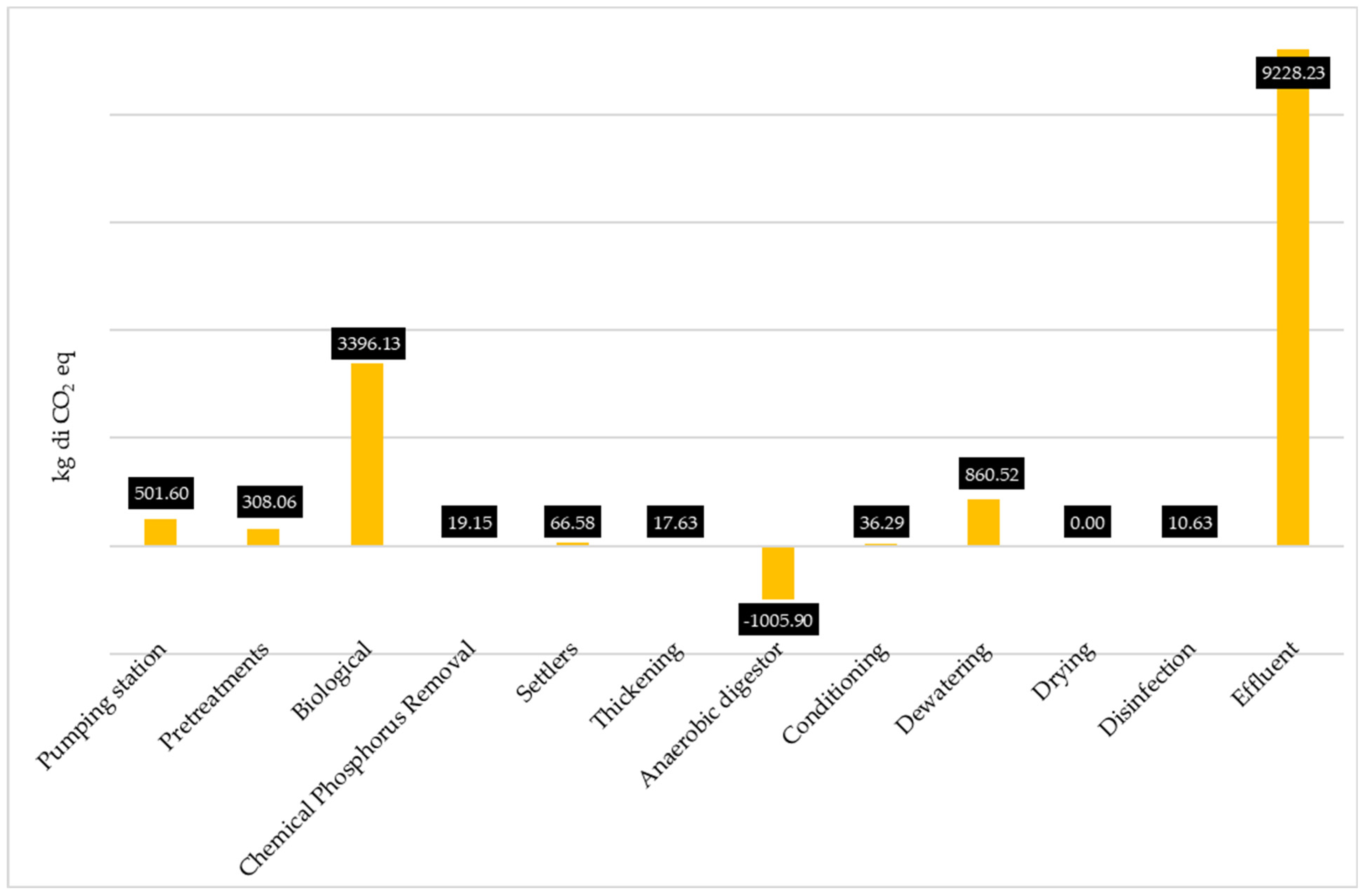
The anaerobic digester reduces the amount of CO₂ released into the atmosphere, as seen by the graph of climate change’s negative impact (Figure 14). The emission of kg CO₂ equivalent from the bioreactor and effluent remains unchanged. Impacts related to potential acidification (PA) and potential eutrophication (PE) also remain unchanged compared to scenario A.

3.4. Comparison between Scenarios A, B, and C

Table 17. Study results and comparable values in the existing literature related to GWP [kgCO₂ equivalent/d], PA [kg SO₂ equivalent/d], and PE [kg PO⁻₄ equivalent/d]—scenario A, B, and C.

Literature	GWP [kgCO2 eq/d]	PA [kg SO2 eq/d]	PE [kg PO−4 eq/d]
Present work—Scenario A	6.02 × 10−1	7.6 × 10−5	2.82 × 10−3
(Tsangas et al. [19])	5.73 × 10−1	3.64 × 10−3	1.40 × 10−3
(Li et al. [5])	6.60 × 10−1	6.34 × 10−3	4.12 × 10−2
(Banti et al. [22])	2.68 × 101	1.15 × 10−2	4.77 × 10−3
Present work—Scenario B	6.66 × 10−1	7.6 × 10−5	2.82 × 10−3
(Ioannou—Ttofa et al. [29])	4.65 × 101	\	\
(Banti et al. [22])	4.96 × 101	1.98 × 10−3	8.60 × 10−4
Present work—Scenario C	5.53 × 10−1	7.6 × 10−5	2.82 × 10−3
(Pasciucco et al. [45])	8.755 × 10−1	2.05 × 10−3	1.55 × 10−2
(Pasqualino et al. [12])	1.19 × 10−1	1.69 × 10−3	1.37 × 10−3

shows the comparison between the three scenarios conducted in this study and the data in the existing literature. Regarding GWP, the obtained results are in accordance with the literature studies; nevertheless, they show lower values for the remaining two categories, PA and PE. In scenario B, the study conducted by Ioannou-Ttofa et al. [29] reports that 97% of the contribution of kg CO₂ equivalent is due to the energy consumption related to the lift pump, the blowers in the pre-aeration tank, and the blowers and backwash pump in the MBR module. The functional unit used corresponds to the one in the present study. Banti et al. [22] show different results to the previous ones, probably due to the different analysis methodologies used. The values of these studies are shown in Table 17. In scenario C, Pasqualino et al. [12] (Table 17) use the same functional unit and system boundaries used in the LCA conducted in this study. Pasciucco et al. [45] (Table 13) consider three different water treatment plants located in central Italy, thus having a geographical location corresponding to that of the plant under analysis. The plant used for comparison with this scenario is WWTP3, which is the only one to use an anaerobic digester. Since the LCIA results are presented in both high and low seasons (HSs and LSs), an average between the two values is considered.

The last stage of the LCA methodology is the interpretation of the results (ISO 14044:2006), in which the most incisive impacts revealed during the study are highlighted. After data input and the construction of an LCA, the different impacts were identified according to the three scenarios analyzed: the first related to a conventional water treatment plant, the second with the implementation of an MBR and finally the third with an anaerobic digester used for the stabilization of the sludges within the conventional plant. The study was based on the functional unit of 1 m³ of influent. The assessment of the impact of the environmental categories considered, i.e., greenhouse effect, acidification, and eutrophication, showed that in all three cases the effluent has the greatest impact in terms of CO₂ equivalent due to the presence of N₂O in the flow. As it is known, this substance has a high conversion factor (298 times greater than that of CO₂ as reported by CML 2001). Direct emissions of N₂O also occur as a result of micro-organism reactions inside the biological reactor, in which there is also the greatest energy consumption due to the presence of highly energy-intensive electromechanical components.

The potential eutrophication category is characterized by two main aspects: effluent discharge and transport. The discharge-related impact is due to the presence of residual P_TOT in the effluent.

Road transport makes the most significant contribution to potential acidification. In fact, emissions related to transport discharges include chemicals such as NO_X, SO₂, and NH₃, which are involved in the acidification phenomenon. As seen in the case of eutrophication, the greatest transport-related load occurs at dewatering, which takes into account the transport of dewatered sludge to the two disposal centers.

Analyzing the results obtained in the three scenarios and comparing them with each other, several considerations emerge as follows:

• Emissions for the GWP category related to biological processes, transport, and effluent do not vary significantly between the considered solutions;
• Among the three scenarios, the acidification and eutrophication categories maintain unchanged values. This is rather obvious because these environmental impacts do not depend on the type of technological solution adopted.

Since emissions from biological processes, transport, and effluent remain practically unchanged in the three scenarios, it is preferable to focus on the environmental loads associated with energy consumption only.

As Figure 15 clearly shows, daily CO₂ emissions are significantly lower in scenario C than in the other two solutions. This reduction is attributable to both lower energy consumption of the equipment in use and to the partial use of energy from renewable sources, such as biogas. In the cases of scenarios A and B, on the other hand, the plant is powered entirely through the national electricity grid.

The adoption of technology under scenario C results in a daily avoided impact of 3935.16 kg of equivalent CO₂ compared to scenario B and 2209.77 kg of equivalent CO₂ compared to scenario A. Projecting these savings over a one-year timeframe results in 1,436,334.758 kg of equivalent CO₂ and 806,567.4078 kg of equivalent CO₂ of avoided impacts, respectively. Figure 15 underlines the long-term effectiveness of the technology proposed by scenario C for minimizing the environmental impact of greenhouse gas emissions.

Substances like pharmaceuticals and toxic compounds have not been considered because they were not present (just traces of pharmaceuticals) in the main flow incoming to the studied plant.

3.5. Sludge Disposal and Management in the Three Scenarios

Sludge is one of the main by-products leaving the plant, therefore it deserves to be analyzed deeply in a specific further LCA study. To ensure the completeness of the study, a short description of the impacts caused by the most used technologies for the sludge disposal is reported.

The most common sludge disposal methods are landfilling, incineration, composting, and land use. Composting is generally carried out by mixing a portion of sludge from WWTP with solid waste, so it was not considered in the study due to the lack of information about the solid waste portion. The analysis was then carried out qualitatively (based on the literature) on the three main technologies that can be used: landfilling, incineration, and land use. The reported values obtained from other authors should be added to the impacts obtained, in particular for the GWP evaluation.

According to the values presented in

Table 18. Comparison between different sludge disposal (landfilling, incineration, and land use) according to [46].

Landfilling	Incineration	Land Use
kg CO2 eq./t DS	kg CO2 eq./t DS	kg CO2 eq./t DS
4322	3124	489

, the worst impact is found when unstabilized sludges are carried to the landfill disposal system due to methane production and for biological activity, incineration has a rather high impact if there is not energy recovery, while land use seems to have the lowest impact in terms of GWP and could then be coupled with effective WWTP management. So, in scenarios A and B, because the sludges are not stabilized, the use of landfill as a final disposal system should have a significant impact on the GWP value. A lower impact could be found in scenario C, where the sludges go through a stabilization process that significantly reduces methane production and biological activities overall. The stabilization process does not influence the GWP expectations for the incineration, while for land use as final disposal, the impact should be greater for the biological activity on the carbonaceous substrate present in the sludges.

4. Conclusions

The European Community’s new guidelines represent a significant step towards the promotion of sustainable and environmentally conscious practices. In the “Green Paper on Integrated Product Policy” COM 2001/68/EC, the European Union officially recognizes the validity and importance of the Life Cycle Assessment (LCA) tool. This endorsement underlines the commitment to a more holistic approach to assessing the environmental impact of products and services.

The new directives not only recognize the importance of LCA, but actively push member countries to implement this tool in service production and processes. The primary objective is to reduce not only atmospheric emissions, but also water and soil pollution while promoting the adoption of innovative and sustainable technologies to limit the use of non-renewable sources.

In the context of this study, the LCA analysis proved to be a particularly suitable tool for evaluating and comparing three distinct scenarios related to wastewater treatment. This methodology makes it possible to assess the emissions produced within pre-determined system boundaries, thus providing a complete picture of the environmental implications of each technology considered.

The comparison of wastewater treatment technologies plays a crucial role in this context, as the sustainable management of water resources is of paramount importance in addressing today’s environmental challenges. Through LCA analysis, the environmental impact of each option can be accurately assessed, enabling an informed and sustainability-oriented choice.

Analyzing the presented scenarios, it is possible to affirm that scenario B, while it is expected to give good removal efficiencies with the use of MBR technology, has high impacts due to high energy consumption to power the used technology. The treatment technology under scenario C involves careful resource management and the introduction of treatment technologies that allow for a decrease in the consumption of non-renewable energy sources, in favor of renewable ones. This makes it possible to use LCA as a decision maker support in the design of new treatment plants. A further step can interest the impact associated with the practical realization of a wastewater plant, where the design choice involving materials and technologies can be improved for the sustainability point of view by means of an LCA analysis.

The use of LCA applied to the management of a WWTP can then be considered a powerful tool to make real-time ratings on the efficiency of the technologies used in the plant or to make sustainable choices on the design of the different treatments to be used for water purification. Even if the sludge treatment and disposal are considered, the LCA approach can be an important help for decision makers, as shown by the fact that a complete process, including digestion followed by a land use disposal, can be more sustainable than other technologies.

This article is going to be used as decision maker support in the analyzed WWTP revamping process. The use of LCA was necessary for the great attention given to DNSH (Do No Significant Harm) in Europe. The LCA methodology, used in this study as an analysis tool for assessing the impacts associated with a WWTP, can be used to enlarge the future research. LCA can be applied to sludge treatment and disposal. LCA application can be used to correctly address disposal choices based on the different impacts linked to composting, landfilling, incineration, and other technologies as briefly shown in this work. A further study of great interest, already implemented and in the final phase, is the application of LCA to the construction steps of a WWTP, with a focus on the plant’s capacity and the used materials.

References

- Ruggerio, C.A. Sustainability and Sustainable Development: A Review of Principles and Definitions. Sci. Total Environ. 2021, 786, 147481. [Google Scholar] [CrossRef] [PubMed]
- Patel, K.; Singh, S.K. A Life Cycle Approach to Environmental Assessment of Wastewater and Sludge Treatment Processes. Water Environ. J. 2022, 36, 412–424. [Google Scholar] [CrossRef]
- IEA—International Energy Agency. World Energy Outlook 2016—Excerpt—Water-Energy Nexus; IEA: Paris, France, 2016. [Google Scholar]
- European Commission. The European Green Deal; European Union: Brussels, Belgium, 2020. [Google Scholar]
- Li, Y.; Xu, Y.; Fu, Z.; Li, W.; Zheng, L.; Li, M. Assessment of Energy Use and Environmental Impacts of Wastewater Treatment Plants in the Entire Life Cycle: A System Meta-Analysis. Environ. Res. 2021, 198, 110458. [Google Scholar] [CrossRef] [PubMed]
- Sappa, G.; Iacurto, S.; Ponzi, A.; Tatti, F.; Torretta, V.; Viotti, P. The LCA Methodology for Ceramic Tiles Production by Addition of MSWI BA. Resources 2019, 8, 93. [Google Scholar] [CrossRef]
- Mancini, G.; Luciano, A.; Bolzonella, D.; Fatone, F.; Viotti, P.; Fino, D. A Water-Waste-Energy Nexus Approach to Bridge the Sustainability Gap in Landfill-Based Waste Management Regions. Renew. Sustain. Energy Rev. 2021, 137, 110441. [Google Scholar] [CrossRef]
- Viotti, P.; Tatti, F.; Rossi, A.; Luciano, A.; Marzeddu, S.; Mancini, G.; Boni, M.R. An Eco-Balanced and Integrated Approach for a More-Sustainable MSW Management. Waste Biomass Valorization 2020, 11, 5139–5150. [Google Scholar] [CrossRef]
- Batuecas, E.; Tommasi, T.; Battista, F.; Negro, V.; Sonetti, G.; Viotti, P.; Fino, D.; Mancini, G. Life Cycle Assessment of Waste Disposal from Olive Oil Production: Anaerobic Digestion and Conventional Disposal on Soil. J. Environ. Manag. 2019, 237, 94–102. [Google Scholar] [CrossRef]
- Allami, D.M.; Sorour, M.T.; Moustafa, M.; Elreedy, A.; Fayed, M. Life Cycle Assessment of a Domestic Wastewater Treatment Plant Simulated with Alternative Operational Designs. Sustainability 2023, 15, 9033. [Google Scholar] [CrossRef]
- Tabesh, M.; Feizee Masooleh, M.; Roghani, B.; Motevallian, S.S. Life-Cycle Assessment (LCA) of Wastewater Treatment Plants: A Case Study of Tehran, Iran. Int. J. Civ. Eng. 2019, 17, 1155–1169. [Google Scholar] [CrossRef]
- Pasqualino, J.C.; Meneses, M.; Abella, M.; Castells, F. LCA as a Decision Support Tool for the Environmental Improvement of the Operation of a Municipal Wastewater Treatment Plant. Environ. Sci. Technol. 2009, 43, 3300–3307. [Google Scholar] [CrossRef]
- Zhang, Q.H.; Wang, X.C.; Xiong, J.Q.; Chen, R.; Cao, B. Application of Life Cycle Assessment for an Evaluation of Wastewater Treatment and Reuse Project—Case Study of Xi’an, China. Bioresour. Technol. 2010, 101, 1421–1425. [Google Scholar] [CrossRef] [PubMed]
- Li, Y.; Luo, X.; Huang, X.; Wang, D.; Zhang, W. Life Cycle Assessment of a Municipal Wastewater Treatment Plant: A Case Study in Suzhou, China. J. Clean. Prod. 2013, 57, 221–227. [Google Scholar] [CrossRef]
- Amores, M.J.; Meneses, M.; Pasqualino, J.; Antón, A.; Castells, F. Environmental Assessment of Urban Water Cycle on Mediterranean Conditions by LCA Approach. J. Clean. Prod. 2013, 43, 84–92. [Google Scholar] [CrossRef]
- Gallego-Schmid, A.; Tarpani, R.R.Z. Life Cycle Assessment of Wastewater Treatment in Developing Countries: A Review. Water Res. 2019, 153, 63–79. [Google Scholar] [CrossRef] [PubMed]
- ISO 14040:1997; Environmental Management-Life Cycle Assessment-Principles and Framework. ISO: Geneva, Switzerland, 1997.
- ISO 14044:2006; Environmental Management-Life Cycle Assessment-Requirements and Guidelines Management Environnemental-Analyse Du Cycle de Vie-Exigences et Lignes Directrices ITeh Standard Preview. ISO: Geneva, Switzerland, 2006.
- Tsangas, M.; Papamichael, I.; Banti, D.; Samaras, P.; Zorpas, A.A. LCA of Municipal Wastewater Treatment. Chemosphere 2023, 341, 139952. [Google Scholar] [CrossRef] [PubMed]
- Corominas, L.; Byrne, D.M.; Guest, J.S.; Hospido, A.; Roux, P.; Shaw, A.; Short, M.D. The Application of Life Cycle Assessment (LCA) to Wastewater Treatment: A Best Practice Guide and Critical Review. Water Res. 2020, 184, 116058. [Google Scholar] [CrossRef] [PubMed]
- Buyukkamaci, N. Life Cycle Assessment Applications in Wastewater Treatment. In Ecological Technologies for Industrial Wastewater Management: Petrochemicals, Metals, Semi-Conductors, and Paper Industries; Apple Academic Press: Palm Bay, FL, USA, 2015; pp. 263–268. ISBN 9781771882866. [Google Scholar]
- Banti, D.C.; Tsangas, M.; Samaras, P.; Zorpas, A. LCA of a Membrane Bioreactor Compared to Activated Sludge System for Municipal Wastewater Treatment. Membranes 2020, 10, 421. [Google Scholar] [CrossRef] [PubMed]
- Adibimanesh, B.; Polesek-Karczewska, S.; Bagherzadeh, F.; Szczuko, P.; Shafighfard, T. Energy Consumption Optimization in Wastewater Treatment Plants: Machine Learning for Monitoring Incineration of Sewage Sludge. Sustain. Energy Technol. Assess. 2023, 56, 103040. [Google Scholar] [CrossRef]
- Aghabalaei, V.; Nayeb, H.; Mardani, S.; Tabeshnia, M.; Baghdadi, M. Minimizing Greenhouse Gases Emissions and Energy Consumption from Wastewater Treatment Plants via Rational Design and Engineering Strategies: A Case Study in Mashhad, Iran. Energy Rep. 2023, 9, 2310–2320. [Google Scholar] [CrossRef]
- Ferrentino, R.; Langone, M.; Fiori, L.; Andreottola, G. Full-Scale Sewage Sludge Reduction Technologies: A Review with a Focus on Energy Consumption. Water 2023, 15, 615. [Google Scholar] [CrossRef]
- Pesqueira, J.F.J.R.; Pereira, M.F.R.; Silva, A.M.T. Environmental Impact Assessment of Advanced Urban Wastewater Treatment Technologies for the Removal of Priority Substances and Contaminants of Emerging Concern: A Review. J. Clean. Prod. 2020, 261, 121078. [Google Scholar] [CrossRef]
- McNamara, G.; Fitzsimons, L.; Horrigan, M.; Phelan, T.; Delaure, Y.; Corcoran, B.; Doherty, E.; Clifford, E. Life Cycle Assessment of Wastewater Treatment Plants in Ireland. J. Sustain. Dev. Energy Water Environ. Syst. 2016, 4, 216–233. [Google Scholar] [CrossRef]
- Machado, A.P.; Urbano, L.; Brito, A.G.; Janknecht, P.; Salas, J.J.; Nogueira, R. Life Cycle Assessment of Wastewater Treatment Options for Small and Decentralized Communities. Water Sci. Technol. 2007, 56, 15–22. [Google Scholar] [CrossRef] [PubMed]
- Ioannou-Ttofa, L.; Foteinis, S.; Chatzisymeon, E.; Fatta-Kassinos, D. The Environmental Footprint of a Membrane Bioreactor Treatment Process through Life Cycle Analysis. Sci. Total Environ. 2016, 568, 306–318. [Google Scholar] [CrossRef] [PubMed]
- Fang, L.L.; Valverde-Pérez, B.; Damgaard, A.; Plósz, B.G.; Rygaard, M. Life Cycle Assessment as Development and Decision Support Tool for Wastewater Resource Recovery Technology. Water Res. 2016, 88, 538–549. [Google Scholar] [CrossRef]
- Piao, W.; Kim, Y.; Kim, H.; Kim, M.; Kim, C. Life Cycle Assessment and Economic Efficiency Analysis of Integrated Management of Wastewater Treatment Plants. J. Clean. Prod. 2016, 113, 325–337. [Google Scholar] [CrossRef]
- Hai, F.I.; Yamamoto, K.; Lee, C.-H. Membrane Biological Reactors: Theory, Modeling, Design, Management and Applications to Wastewater Reuse; IWA Publishing: London, UK, 2019; ISBN 9781780400655. [Google Scholar]
- Mahmood, S.; Rahman Hemdi, A.; Zameri, M.; Saman, M.; Yusof, N.M. Sustainability Assessment of Membrane System for Wastewater Treatment: A Review and Further Research. In Proceedings of the 20th CIRP International Conference on Life Cycle Engineering, Singapore, 17–19 April 2013. [Google Scholar]
- Raghuvanshi, S.; Bhakar, V.; Sowmya, C.; Sangwan, K.S. Waste Water Treatment Plant Life Cycle Assessment: Treatment Process to Reuse of Water. Procedia CIRP 2017, 61, 761–766. [Google Scholar] [CrossRef]
- Santucci, V.G.; Baldassarre, G.; Mirolli, M. Intrinsic Motivation Mechanisms for Competence Acquisition. In Proceedings of the 2012 IEEE International Conference on Development and Learning and Epigenetic Robotics (ICDL), San Diego, CA, USA, 7–9 November 2012. [Google Scholar]
- Parkin, G.F.; Owen, W.F. Fundamentals of Anaerobic Digestion of Wastewater Sludges. J. Environ. Eng. 1986, 112, 867–920. [Google Scholar] [CrossRef]
- Osorio, F.; Torres, J.C. Biogas Purification from Anaerobic Digestion in a Wastewater Treatment Plant for Biofuel Production. Renew. Energy 2009, 34, 2164–2171. [Google Scholar] [CrossRef]
- Bartram, D.; Short, M.D.; Ebie, Y.; Farkaš, J.; Gueguen, C.; Peters, G.M.; Zanzottera, N.M.; Karthik, M. Volume 5: Waste—Chapter 6 Wastewater Treatment and Discharge. In Refinement to the 2006 IPCC Guidelines for National Greenhouse Gas Inventories; IPCC: Geneva, Switzerland, 2019; pp. 6.1–6.28. [Google Scholar]
- Yoshida, H.; Mønster, J.; Scheutz, C. Plant-Integrated Measurement of Greenhouse Gas Emissions from a Municipal Wastewater Treatment Plant. Water Res. 2014, 61, 108–118. [Google Scholar] [CrossRef]
- Doorn, M.; Treatment, W.; Guidelines, I.; Irving, W.; Greenhouse, N.; Inventories, G. Chapter 6 Wastewater Treatment and Discharge. In 2006 IPCC Guidelines for National Greenhouse Gas Inventories; IPCC: Geneva, Switzerland, 2006. [Google Scholar]
- Boiocchi, R.; Viotti, P.; Lancione, D.; Stracqualursi, N.; Torretta, V.; Ragazzi, M.; Ionescu, G.; Rada Elena, C. A Study on the Carbon Footprint Contributions from a Large Wastewater Treatment Plant. Energy Rep. 2023, 9, 274–286. [Google Scholar] [CrossRef]
- Çankaya, S.; Pekey, B. Evaluating the Environmental and Economic Performance of Biological and Advanced Biological Wastewater Treatment Plants by Life Cycle Assessment and Life Cycle Costing. Environ. Monit. Assess. 2024, 196, 373. [Google Scholar] [CrossRef] [PubMed]
- Petrarca, S.; Cogliani, E.; Spinelli, F. La Radiazione Solare Globale Al Suolo in Italia; ENEA: Stockholm, Sweden, 2000. [Google Scholar]
- MITE. Linee Guida in Materia di Impianti Agrivoltaici; Ministero Della Transizione Ecologica—Dipartimento per L’energia: Roma, Italy, 2022; 39p. [Google Scholar]
- Pasciucco, F.; Pecorini, I.; Iannelli, R. A Comparative LCA of Three WWTPs in a Tourist Area: Effects of Seasonal Loading Rate Variations. Sci. Total Environ. 2023, 863, 160841. [Google Scholar] [CrossRef] [PubMed]
- Zhao, G.; Liu, W.; Xu, J.; Huang, X.; Lin, X.; Huang, J.; Li, G. Greenhouse Gas Emission Mitigation of Large-Scale Wastewater Treatment Plants (WWTPs): Optimization of Sludge Treatment and Disposal. Pol. J. Environ. Stud. 2021, 30, 955–964. [Google Scholar] [CrossRef] [PubMed]
Figure 1.
Activated sludge plant scheme—scenario A.
Figure 2.
Activated sludge plant scheme with MBR—scenario B.
Figure 3.
Activated sludge plant scheme with anaerobic digester and photovoltaic system—scenario C.
Figure 4.
Energy consumption [%] related to the number of electromechanical components in the different sections of the plant—scenario A.
Figure 5.
CO2 emissions [%] related to energy consumption, transportation, and biological reactions—scenario A.
Figure 6.
Global warming potential (GWP) [kgCO2 equivalent/d]—scenario A.
Figure 7.
Energy consumption [%]—scenario B.
Figure 8.
CO2 emissions [%] related to energy consumption, transportation, and biological reactions—scenario B.
Figure 9.
Global warming potential (GWP) [kgCO2 equivalent/d]—scenario B.
Figure 10.
Energy consumption [kWh/d per F.U.]—scenario C.
Figure 11.
CO2 Emissions related to energy consumption, transportation and biological reactions [%]—scenario C.
Figure 12.
Simulation outputs—monthly energy output from fix-angle PV system.
Figure 13.
Simulation outputs—battery performance for off-grid PV system (In green are the days when the battery is always full, and in red when it is empty. As can be seen from the graph, since there are no histograms shown in red, the battery is never empty).
Figure 14.
Global warming potential (GWP) [kgCO2 equivalent/d]—scenario C.
Figure 15.
Comparison of GWP in the three different scenarios on a daily basis (related to energy consumption) [kg CO2 eq].