Research on Annual Runoff Prediction Model Based on Adaptive Particle Swarm Optimization–Long Short-Term Memory with Coupled Variational Mode Decomposition and Spectral Clustering Reconstruction

Abstract

Accurate medium- and long-term runoff prediction models play crucial guiding roles in regional water resources planning and management. However, due to the significant variation in and limited amount of annual runoff sequence samples, it is difficult for the conventional machine learning models to capture its features, resulting in inadequate prediction accuracy. In response to the difficulties in leveraging the advantages of machine learning models and limited prediction accuracy in annual runoff forecasting, firstly, the variational mode decomposition (VMD) method is adopted to decompose the annual runoff series into multiple intrinsic mode function (IMF) components and residual sequences, and the spectral clustering (SC) algorithm is applied to classify and reconstruct each IMF. Secondly, an annual runoff prediction model based on the adaptive particle swarm optimization–long short-term memory network (APSO-LSTM) model is constructed. Finally, with the basis of the APSO-LSTM model, the decomposed and clustered IMFs are predicted separately, and the predicted results are integrated to obtain the ultimate annual runoff forecast results. By decomposing and clustering the annual runoff series, the non-stationarity and complexity of the series have been reduced effectively, and the endpoint effect of modal decomposition has been effectively suppressed. Ultimately, the expected improvement in the prediction accuracy of the annual runoff series based on machine learning models is achieved. Four hydrological stations along the upper reaches of the Fen River in Shanxi Province, China, are studied utilizing the method proposed in this paper, and the results are compared with those obtained from other methods. The results show that the method proposed in this article is significantly superior to other methods. Compared with the APSO-LSTM model and the APSO-LSTM model based on processed annual runoff sequences by single VMD or Wavelet Packet Decomposition (WPD), the method proposed in this paper reduces the RMSE by 40.95–80.28%, 25.26–57.04%, and 15.49–40.14%, and the MAE by 24.46–80.53%, 16.50–59.30%, and 16.58–41.80%, in annual runoff prediction, respectively. The research has important reference significance for annual runoff prediction and hydrological prediction in areas with data scarcity.

1. Introduction

In recent years, the frequent occurrence of extreme climate events has exerted a profound influence on the global water cycle [1]. Extreme precipitation [2], extreme drought [3], and extreme flooding [4] pose a great threat to human lives, property, and safety. An accurate runoff forecast plays a vital role in water resource management. By predicting the runoff for the next year, it can help decision makers better plan the utilization and distribution of water resources, thereby coping with possible extreme climate events such as droughts or floods, preventing and mitigating the corresponding disasters. Therefore, an increasing number of scholars [5,6] have conducted detailed studies on the methods related to runoff prediction. However, due to the extremely complex mechanism of the non-linear and non-stationary nature of runoff series [7], it is still an untoward task to forecast medium- and long-term runoff accurately.

Currently, the widely employed models for runoff forecasting include physically based hydrological models and data-driven hydrological models [8]. The hydrological models deriving from a physical process generally combine the processes of meteorological elements, and utilize the traditional runoff generation as well as confluence theory to achieve the runoff prediction. The drawbacks of the methods are quite apparent, such as the difficulty in acquiring meteorological data and the presence of numerous empirical parameters that need to be determined in traditional hydrological theories [9]. In contrast, there is no need for the hydrological models based on data-driven, with machine learning, model ideas to require the explicit hydrological physical process, instead, just simply combine precipitation, evapotranspiration, and runoff data to achieve runoff prediction. The hydrological models based on data-driven model ideas can be further divided into two types, namely, those combined with thoughts of mathematical statistics [10] and the machine learning model ideas [11]. Among them, the performances of machine learning models represented by the LSTM model [12], support vector machine (SVM) model [13], and extreme gradient boosting (XGB) model [14] have consistently exceeded the hydrological models based on physical processes in medium- and long-term runoff forecasting. Therefore, this type of method has gained favor among numerous scholars.

To further improve the runoff prediction ability built upon machine learning models, the current studies mainly focus on two aspects, on the one hand, optimizing and improving various parameters and mechanisms within machine learning models, starting from the internal mechanisms. Examples are employing optimization algorithms like particle swarm optimization to fine-tune the sensitive parameters of machine learning models [15], adding appropriate attention mechanisms [8,16], and incorporating multiple time scales into machine learning models [17]. On the other hand, starting from reducing the complexity of data by integrating the “decomposition–prediction–reconstruction” strategy in the field of time series prediction [18,19], complex sequences are partitioned into multiple intrinsic mode function (IMF) components with simple characteristics and residual sequences established on certain mathematical rules. Subsequently, all of the IMFs can be predicted and reconstructed to obtain the final prediction results. The “decomposition–prediction–reconstruction” strategy can further explore the data characteristics of runoff series, thereby effectively improving forecast accuracy [7,20]. Nevertheless, the related research findings indicated that [21,22] the application of decomposition methods introduced a boundary effect to the sequences, limiting the further improvement in prediction accuracy to some extent. Aiming at this issue, periodic extension and quadratic decomposition methods have been proposed and applied [23,24,25], achieving relatively favorable results to a certain extent. However, in regard to annual runoff forecasting, the full potential of the two methods remains underutilized. The challenge lies in capturing the periodic traits of annual runoff series, primarily due to the inherent limitation in the length of series. Meanwhile, the direct extending may result in data distortion after extension. Conversely, making use of the quadratic decomposition method may exacerbate the endpoint problem. Therefore, determining the appropriate preprocessing methods for limited-length, complex, and non-stationary original annual runoff series to effectively extract their features before forecasting becomes pivotal in further enhancing prediction accuracy based on machine learning models. As the research deepens, it is found that by combining clustering algorithms, the finite length time series can be decomposed into IMF components with simple features; at the same time, the endpoint effect problem accompanying the decomposition can be reduced, which aligns well with the requirements of addressing the problem outlined in this article.

On account of this background, the clustering algorithm is employed to classify and reconstruct the decomposed annual runoff IMFs in this research, and a new annual runoff prediction model, termed VMDSC-APSO-LSTM, is constructed based on the basic prediction model APSO-LSTM. On one side, the use of clustering algorithms to process the annual runoff IMFs can avoid the length requirement of runoff sequences by applying periodic extension methods. On the other side, the number of reconstructed annual runoff IMFs is reduced, which is beneficial for mitigating the boundary effects induced by decomposition algorithms.

In summary, to improve the prediction accuracy of annual runoff series, based on the APSO-LSTM model, taking advantage of the variational mode decomposition (VMD) method, and aiming to reduce the endpoint effects, a comprehensive annual runoff prediction model, VMDSC-APSO-LSTM, is proposed in this study, which couples the spectral clustering (SC) algorithm and VMD method. Taking four hydrological stations in the upper reaches of the Fenhe River in China as research objects, the annual runoff prediction results built upon VMDSC-APSO-LSTM are compared and analyzed with the other three models to examine the effectiveness and applicability of the proposed method.

Considering the aforementioned discussion, the novelty of this study can be summarized in three parts. Firstly, a method for extracting complex time series features by coupling the SC algorithm and VMD method is proposed. Secondly, a comprehensive annual runoff prediction model, VMDSC-APSO-LSTM, with the help of the SC algorithm and VMD method is put forward. Finally, the effectiveness and superiority of the proposed method is confirmed via a case study. In addition, the research findings can be applied to annual runoff forecasts for other regions and even to forecasting tasks in other fields with the time series, which have the characteristics of significant spatial heterogeneity and limited sequence length.

2. Methodology

2.1. VMD Model

The VMD model is an adaptive, completely non-recursive approach to sequence decomposition proposed by Dragomiretskiy et al. [26]. This method can effectively reduce the phenomenon of “modal confusion” in empirical modal-type algorithms, which demonstrates the superior performance in non-stationary and non-linear complex signal sequences [27]. Therefore, in this study, the method is utilized to decompose the annual runoff series and extract key information from the complex series. The primary principles of the model are as follows:

• Establish a variational problem: The marginal spectrum of each modal function a_k(t) is solved by applying the Hilbert transform; subsequently, the exponential term of each modal center frequency bk is incorporated to complete the modulation of the fundamental band of a_k(t). Finally, the bandwidth of each mode is determined by using the Gaussian smoothing method, and a variational problem with constraints is formulated as follows:

$$\left\{\begin{array}{c}\underset{\left\{a_k\right\},\{b_k\mid }{min}T=\sum _k{‖{\partial }_t[(\delta (t)+\frac{j}{\pi t})*a_k(t)]e^{-j{b}_{k^t}}‖}_2^2,k=\mathrm{1,2},\cdots ,L\\ \mathrm{s}.\mathrm{t}.\sum _k{a}_k=f\left(t\right)\end{array}\right.$$

(1)

where T represents the objective function of the variational problem. a_k denotes the k-th modal function. b_k signifies the center frequency of the k-th modal function. δ(t) belongs to the Dirac distribution. $(\delta (t)+\frac{j}{\pi t})$ means a single spectrum, and f(t) is the original runoff sequence.

2.

Solve the variational problem: The aforementioned constrained problem is converted to an unconstrained problem by employing penalty factor α and Lagrange multiplier λ:

$$L\left(\left\{a_k\right\},\left\{b_k\right\},\lambda \right)=\alpha {\sum }_k{‖{\partial }_t[(\delta (t)+\frac{j}{\pi t})\mathrm{*}{a}_k(t)]e^{-j{b}_{k}t}‖}_2^2+\Vert f\left(t\right)-{\sum }_k{a}_k\left(t\right){\Vert }_2^2$$

$$+\langle \lambda ,f\left(t\right)-{\sum }_k{a}_k\left(t\right)\rangle$$

(2)

The Parseval theorem is a fundamental theorem in signal processing and a Fourier analysis. According to Parseval’s theorem in a Fourier transform, it can be found that the energy of the signal is equivalent in both the time and frequency domains. Therefore, the problem in the time domain can be solved in the frequency domain. For a signal f(t) and its Fourier transform F(ω), the Parseval theorem can be expressed as

$${\int }_{-\mathrm{\infty }}^{\mathrm{\infty }}{\left|f\left(t\right)\right|}^{2}dt=\frac{1}{2\pi }{\int }_{-\mathrm{\infty }}^{\mathrm{\infty }}{\left|F\left(\omega \right)\right|}^{2}d\omega$$

(3)

By using the Parseval theorem, the spectral characteristics of a signal can be observed from a frequency domain perspective. In short, such transformations enable the previously insignificant features of runoff sequences to be displayed in the complex field in a spectral manner, making it easier for further mining in deep learning.

The modal function ${\widehat{a}}_k^{n+1}$, center frequency ${\widehat{b}}_k^{n+1}$, and Lagrange multiplier ${\widehat{\lambda }}^{n+1}$ in Equation (2) are iteratively updated through the alternating-direction multiplier method, and the iterative formulae are as follows:

$$\left\{\begin{array}{l}{\widehat{a}}_k^{n+1}=\frac{\widehat{f}\left(b\right)-\sum _{i>k}{\widehat{a}}_i^n\left(b\right)+\frac{{\widehat{\lambda }}^n\left(b\right)}{2}}{1+2\alpha {\left(b-b_k^n\right)}^2}\\ {\widehat{b}}_k^{n+1}=\frac{{\int }_0^{\infty }b{\left|{\widehat{a}}_k^{n+1}\left(b\right)\right|}^{2}db}{{\int }_0^{\infty }{\left|{\widehat{a}}_k^{n+1}\left(b\right)\right|}^{2}db}\\ {\widehat{\lambda }}^{n+1}={\widehat{\lambda }}^n\left(b\right)+\tau \left(\widehat{f}\left(b\right)-{\displaystyle \sum _k}{\widehat{a}}_k^{n+1}\left(b\right)\right)\end{array}\right.$$

(4)

where $\widehat{ }$ is the frequency domain form corresponding to the Fourier transform of the signal. τ denotes the noise tolerance. n stands for the number of iterations.

The expression for the iteration termination condition is the following:

$$\frac{\sum _{k=1}^k{‖{\widehat{a}}_k^{n+1}-{\widehat{a}}_k^n‖}_2^2}{{‖{\widehat{a}}_k^n‖}_2^2}<\epsilon$$

(5)

in which ε represents the convergence tolerance error, which is set to 10⁻⁷ in this study.

2.2. Spectral Clustering (SC) Model

Although the VMD model is a non-recursive decomposition method, the truncation of the signal and the use of the Hilbert transform can lead to certain boundary effects [21]. For the sake of suppressing the error accumulation resulting from this effect in the prediction process, it is proposed in this study to classify each IMF after decomposition by the clustering model, and then integrate the IMFs in groups in order to reduce the prediction numbers of endpoints for the prediction model, thereby minimizing the error accumulation. Considering the large number of data points in each IMF, the mean and variance are selected as the eigenvalues of each IMF in the clustering model to form the point set.

The common clustering algorithms can be mainly classified into six categories, namely, the prototype clustering, density clustering, hierarchical clustering, grid clustering, model clustering, and spectral clustering. Among them, the SC is a method of clustering without requiring the clustering object to have a convex sphere or other specific shape. Considering the unknown nature of each IMF sample after modal decomposition, the SC algorithm is adopted to classify the IMFs in this paper.

The SC is a clustering algorithm evolved from the graph theory. The main idea of SC is to treat all data as points in space initially, where these points can be connected to each other by edges. The edge weight value between two points that are farther away is lower, whereas it is higher for closer points. Subsequently, by slicing the graph composed of all data points, make the sum of edge weights between different subgraphs after slicing as low as possible, while making the sum of edge weights within subgraphs as high as possible, and thereby the data point clustering can be achieved. The principle of SC is as follows:

First of all, suppose the weight between two points is ω_ij; then, for any point, the corresponding degree d_i can be defined as the weights’ sum of all edges connected to it, which can be expressed as

$$d_i=\sum _{j=1}^n{\omega }_{ij}$$

(6)

Define the subset of point set V as A. The sum of the degrees for all vertices in subset A is denoted by vol(A):

$$vol\left(\mathit{A}\right)=\sum _{i\in A}{d}_i$$

(7)

The degree matrix D can be constructed according to the definition of each point. Only the main diagonal has values in the matrix D. The expression of matrix D is

$$\mathit{D}=\left(\begin{array}{ccc}\begin{array}{cc}{d}_1& \end{array}& & \\ \begin{array}{cc}& d_2\end{array}& & \\ \begin{array}{cc}\begin{array}{c}\\ \end{array}& \begin{array}{c}\\ \end{array}\end{array}& \begin{array}{c}\ddots \\ \end{array}& \begin{array}{c}\\ d_n\end{array}\end{array}\right)$$

(8)

Secondly, through calculating the similarity matrix S formed by these points, the adjacency matrix W can be obtained. The exact calculation methods of the similarity matrix S and adjacency matrix W will not be extensively discussed here, and the detailed procedure can be found in Reference [28]. Consequently, the Laplacian matrix L can be calculated with the following expression:

$$\mathit{L}=\mathit{D}-\mathit{W}$$

(9)

Finally, the indicator vector h_j is introduced and the NCut is performed, in which h_j is an n-dimensional vector, which can be calculated by transforming it into an optimization problem:

$${\mathit{h}}_j=\left\{\begin{array}{l}0,v_i\notin {\mathit{A}}_{\mathit{j}}\\ \frac{1}{\sqrt{vol\left({\mathit{A}}_{\mathit{j}}\right)}},v_i\in {\mathit{A}}_{\mathit{j}}\end{array}\right.$$

(10)

$$\left\{\begin{array}{l}NCut\left({\mathit{A}}_1,{\mathit{A}}_2,\dots ,{\mathit{A}}_{\mathit{k}}\right)={\displaystyle \sum _{i=1}^k}{\mathit{h}}_{\mathit{i}}^{\mathit{T}}\mathit{L}{\mathit{h}}_{\mathit{i}}={\displaystyle \sum _{i=1}^k}{\left({\mathit{H}}^{\mathit{T}}\mathit{L}\mathit{H}\right)}_{ii}\\ \underset{H}{\underbrace{\mathit{arg}min}}={\displaystyle \sum _{i=1}^k}{\left({\mathit{H}}^{\mathit{T}}\mathit{L}\mathit{H}\right)}_{ii}\\ s.t.{\mathit{H}}^{\mathit{T}}DH=I\end{array}\right.$$

(11)

where v_i represents the points in the point set V. I is the unit diagonal matrix. H denotes the optimal indicator vector.

The k-means clustering algorithm is chosen as the base algorithm for SC. The k-means clustering is performed on the points in vector H to obtain the final result of SC.

2.3. APSO-LSTM Model

The LSTM model is a recurrent neural network (RNN) that is suitable for capturing important event dependencies with large intervals in sequential data. The model overcomes the issues of gradient vanishing and exploding in the hidden layer variables of RNN. The implicit state of LSTM includes the implicit layer variables and the memory cells. The memory cells of LSTM are illustrated in Figure 1. In this study, a Dropout layer is set in the LSTM model to reduce the model’s excessive dependence on training data and decrease the risk of model overfitting.

Related studies [29,30,31] have shown that utilizing heuristic optimization algorithms to optimize the parameters of the LSTM model can effectively improve their accuracy in runoff prediction. The particle swarm optimization (PSO) is a population intelligence optimization algorithm inspired by the study of bird flocking behavior. The basic idea of the PSO algorithm revolves around finding the optimal solution through collaboration and information sharing among individuals in a population. The main process is to find the optimal solution by iteration after generating a series of random particles (random solutions). In each iteration, the particle updates their positions by constantly approaching the local and global optima. After obtaining the local and global optima, the particle updates the velocities and positions by Equations (12) and (13):

$$v_i\left(t+1\right)=\omega v_i\left(t\right)+c_1\times r_1\times \left(b_{pi}-x_i\left(t\right)\right)+c_2\times r_2\times \left(b_{gi}-x_i\left(t\right)\right)$$

(12)

$$x_i\left(t+1\right)=x_i\left(t\right)+v_i\left(t+1\right)$$

(13)

where i represents the number of particles, i = 1, 2, …, N. v_i(t) means the velocity of the ith particle at time t. v_i(t + 1) denotes the velocity of the ith particle at time t + 1. c₁ and c₂ are learning factors. r₁ and r₂ symbolize random numbers between 0 and 1. b_pi and b_gi signify the local and global optima, respectively. x_i(t) is the position of the ith particle at time t. x_i(t + 1) connotes the position of the ith particle at time t + 1. Typically, the maximum velocity of v_i(t) is expressed as v_max. When the velocity reaches its maximum value, v_i(t) = v_max.

To better obtain optimization results and prevent them from falling into local optima, some scholars have made improvements to the PSO algorithm [32,33]. For example, an inertia factor ω, which belongs to (0, 1), is introduced to construct an adaptive weighted particle swarm optimization algorithm (APSO). Generally, as the weight value increases, the global optimization ability strengthens while the local optimization ability diminishes. Conversely, as the weight value decreases, the global optimization ability weakens, and the local optimization ability strengthens. For optimal minimization function problems, the update of ω primarily follows the subsequent strategy:

$$\omega =\left\{\begin{array}{c}{\omega }_{min}+\left({\omega }_{max}-{\omega }_{min}\right)\frac{f-f_{min}}{\overline{f}-f_{min}}, f\le \overline{f}\\ f_{max}, f>\overline{f}\end{array}\right.$$

(14)

where ω_min stands for the minimum value of weight, which is set to 0.4. ω_max denotes the maximum value of weight, and the value is 0.9. f is the fitness value of each particle. $\overline{f}$ represents the average fitness value of all particles. f_max is the maximum value of particle fitness. f_min indicates the minimum value of particle weight.

Due to the sensitivity of certain parameters in the LSTM model during actual training, the APSO algorithm is utilized for the optimization of sensitive parameters in LSTM, and the range of each optimization parameter is shown in

Table 1. Preferred Range of Parameters.

Name of Parameters	Meaning of Parameters	Type of Parameters	Range of Values
Learning rate	Initial learning rate	float	[0.001, 0.1]
LSTM layer	Number of LSTM neurons	int	[20, 200]
Max epochs	Maximum number of iterations	int	[20, 200]

.

The APSO algorithm can effectively avoid the objective function falling into a local optimal solution, premature maturity, and convergence during the optimization process. Using the mean square error (MSE) between predicted and measured values as the objective function, an APSO-LSTM annual runoff prediction model is constructed. The process is outlined in Figure 2, and the main steps are as follows:

• Initialization of model parameters: The initial matrix of each optimization parameter in the LSTM algorithm is constructed, and the initial values of other insensitive parameters, population size, population dimension, learning factor, etc., in the APSO algorithm are determined.
• The particle populations X (learning rate, LSTM layer, max epochs) are randomly generated, and the initial velocity and initial position of the particles are defined.
• The values of LSTM parameters are assigned. The model networks under different parameters are trained, and each training process is recorded.
• According to the fitness function, the optimal particle fitness value is selected by calculating and comparing the fitness value of each particle. The velocity and position of the particle itself are updated according to Equations (12) and (13), respectively.
• When the selected maximum number of iterations has been reached, the minimum value of MSE at this time is picked as the optimization result of the objective function. The optimal particle population location is the output. The obtained parameters are assigned to the LSTM model. The trained optimization model is adopted to predict the runoff volume, and then the prediction results can be achieved.

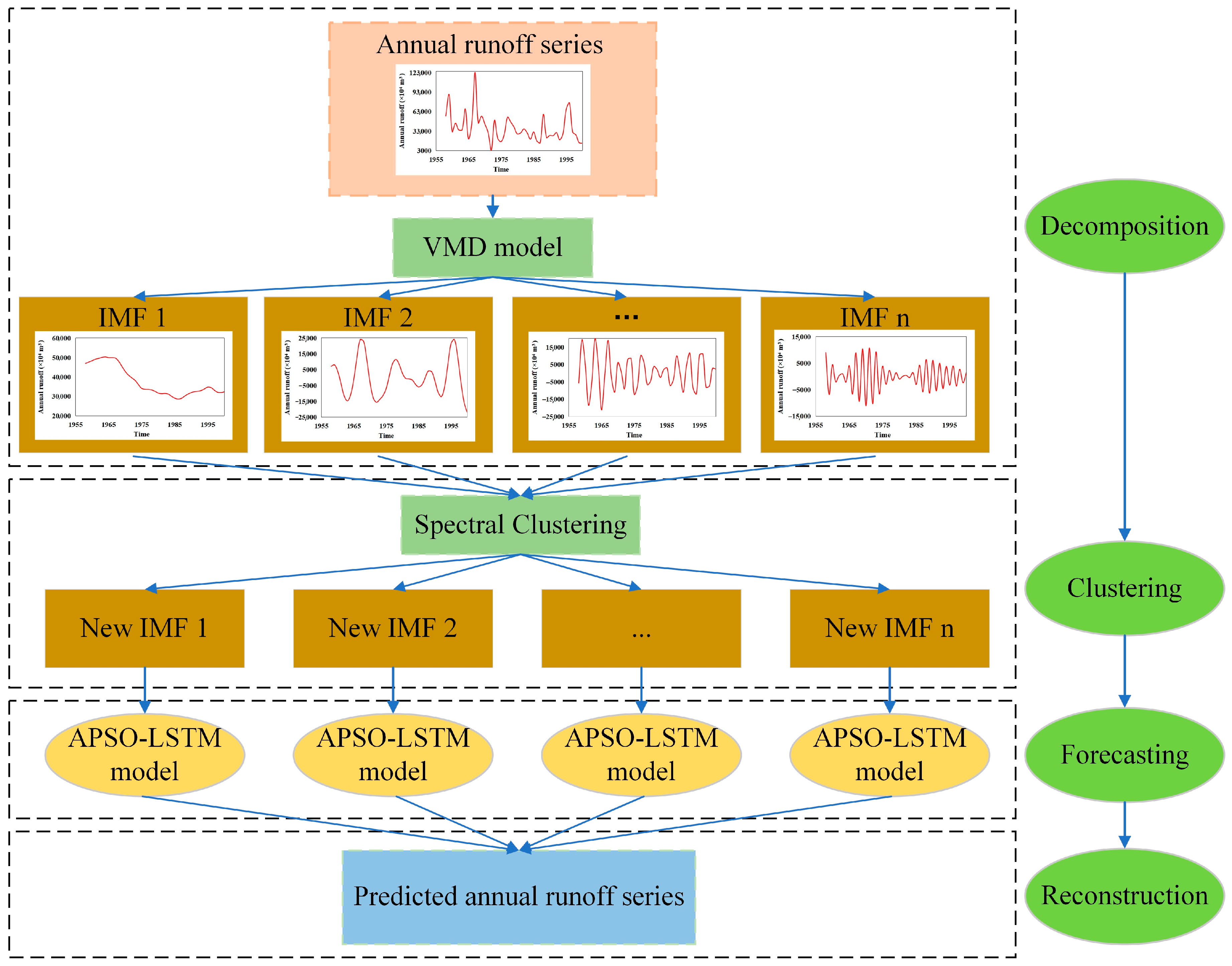
2.4. VMDSC-APSO-LSTM Model

Integrating the advantages of various basic methods mentioned above with the purpose of solving the significant boundary effect question of VMD in a small sample sequence, a new annual runoff prediction model based on decomposition and clustering is proposed in this paper, namely, the VMDSC-APSO-LSTM model. The VMDSC-APSO-LSTM model leverages VMD to extract key feature information from the runoff sequence, aggregates the initial IMFs by SC, and forecasts and integrates the IMFs through APSO-LSTM. The structure of the VMDSC-APSO-LSTM model is depicted in Figure 3.

3. Evaluation of the Model

For a comparative analysis of the accuracy for the proposed model, VMDSC-APSO-LSTM, in this study, three additional models, APSO-LSTM, VMD-APSO-LSTM, and WPD-APSO-LSTM, are added for comparison, and the models are assigned with numbers S4, S1, S2, and S3, respectively, as outlined in

Table 2. Implication of each model.

Serial Number	Model	Implication
S1	APSO-LSTM	Optimization of long short-term memory network model by adaptive particle swarm optimization
S2	VMD-APSO-LSTM	Optimization of long short-term memory network model by adaptive particle swarm optimization based on variational mode decomposition and reconstruction
S3	WPD-APSO-LSTM	Optimization of long short-term memory network model by adaptive particle swarm optimization based on wavelet decomposition and reconstruction
S4	VMDSC-APSO-LSTM	Optimization of long short-term memory network model by adaptive particle swarm optimization based on variational mode decomposition and spectral clustering.

. Among them, the APSO-LSTM model is an improved machine learning model leveraging optimization algorithms, serving as the foundational model in this study. The VMD-APSO-LSTM model is the focus of improvement in this work, with the enhanced model being the VMDSC-APSO-LSTM model proposed in this research. To further examine the effectiveness of the proposed VMDSC-APSO-LSTM model in solving boundary effects, the WPD-APSO-LSTM model is introduced as a control.

The Nash efficiency coefficient (NSE), root mean square error (RMSE), and mean absolute error (MAE) are selected as evaluation indicators for the models, while each evaluation indicator is calculated as follows:

$$\mathrm{N}\mathrm{S}\mathrm{E}=1-\frac{\sum _{t=1}^n{\left(Q_0\left(t\right)-Q_p\left(t\right)\right)}^2}{\sum _{t=1}^n{\left(Q_0\left(t\right)-{\overline{Q}}_o\right)}^2}$$

(15)

$$\mathrm{R}\mathrm{M}\mathrm{S}\mathrm{E}=\sqrt{\frac{1}{n}{\sum }_{t=1}^n{\left(Q_0\left(t\right)-Q_p\left(t\right)\right)}^2}$$

(16)

$$\mathrm{M}\mathrm{A}\mathrm{E}=\frac{1}{n}{\sum }_{t=1}^n\left|Q_0\left(t\right)-Q_p\left(t\right)\right|$$

(17)

where Q₀(t) is the measured annual runoff volume, m³. Q_p(t) denotes the predicted annual runoff volume, m³. n represents the number of years in the test period.

4. Application and Analysis

4.1. Study Area and Data

Fenhe River, the second largest tributary of the Yellow River, China, is depicted in Figure 4. The four hydrological stations located in the upper reaches of the Fenhe River basin, namely, Zhaishang Station, Lancun Station, Fenhe Reservoir Station, and Shangjingyou Station, are utilized as the subjects of study. The collected annual runoff series measured at each hydrological station from 1958 to 2000 are divided into a training set and testing set, with the training set from 1958 to 1994 and the testing set from 1995 to 2000. To prevent the leakage of training set information, the training set is further divided into a new training set and validation set [34]. The new training set is from 1958 to 1988, and the validation set is from 1989 to 1994.

4.2. Decomposition of Annual Runoff Series

It is shown from related work [35] that the sensitive parameters of the VMD model are mainly the number of the decomposition layers K and the penalty factor α. When K is chosen appropriately, the components decomposed by the VMD method can reflect the frequency components contained in the original signal. If the selection of K is not proper, the under-decomposition or over-decomposition phenomenon will occur. Regarding the parameter α, as the corresponding value increases, the decomposition convergence speed of the VMD model tends to initially accelerate and then decelerate. However, the value of α is not a standard proportional or inverse relationship with the running speed of the model. At the same time, a higher value of α reduces the likelihood of a modal confounding occurrence in the results of VMD decomposition.

To sum up, it is necessary for this study to first determine the value of α. The manual tuning method is used to ensure that the value of α is increased by a certain gradient, when the number of decomposition layers is constant. The last α value is determined as the optimal penalty factor while the average absolute error between the reconstructed data and the original data appears to increase. The optimal α value of each station is shown in

Table 3. Table of values for penalty coefficient $\alpha$.

Station	Zhaishang Station	Lancun Station	Fenhe Reservoir Station	Shangjingyou Station
$\alpha$	200	300	900	800

.

The main methods for determining the number of decomposition layers K are the empirical value method and the center frequency method [36]. The center frequency method is adopted in this study and the process to determine the number of decomposition layers at each station is shown in Figure 5.

From Figure 5, it can be seen that as the number of decomposition layers increases, the center frequencies of each IMF are gradually closer to each other. For the Zhaishang Station, when the number of decomposition layers is set to 5, the center frequency of IMF5 is 0.4634; as the number of decomposition layers turns to 6, the center frequency of IMF6 equals to 0.4720. The center frequency of the IMF increases less than 0.01, which indicates that when the runoff sequence of Zhaishang Station is decomposed to the fifth layer, the feature information contained in the sequence can be basically extracted, and if the number of decomposition layers is increased continuously, the phenomenon of “modal mixing” may appear. Therefore, for the sequence of Zhaishang Station, five is selected as the number of decomposition layers. Similarly, by analyzing the runoff series of other stations, it is found that the runoff sequence of each station is optimized when the number of decomposition layers is five.

Combining the parameters determined above, the annual runoff series for the four stations are decomposed, respectively, and the results are depicted in Figure 6.

4.3. Clustering Grouping of IMFs

In this research, the adjacency matrix in the SC algorithm is calculated by employing the Gaussian kernel function radial basis function (RBF). For the standard deviation of RBF, the integer value of the average standard deviation of the clustering points is used. After multiple adjustment experiments, the number of categories for clustering is consistently determined to be three. When each parameter is determined, the decomposition results of each station are analyzed by SC, setting the IMF mean as the horizontal coordinate and the variance as the vertical coordinate. The results are illustrated in Figure 7.

It is seen from Figure 7a that, for the Zhaishang Station, IMF1 and IMF3 are the first category, IMF2 and IMF4 are the second category, and IMF5 is the third category. With regard to the Lancun station, IMF1 and IMF2 belong to the first category, IMF3 and IMF4 are the second category, and IMF5 enters into the third category, as shown in Figure 7b. When the Fenhe Reservoir Station is referred, IMF1 occupies the first category, IMF2 and IMF4 take up the second category, and IMF3 and IMF5 are the third category, as shown in Figure 7c. With respect to the Shangjinyou Station, IMF1 becomes the first category, IMF2 and IMF4 turn into the second category, and IMF3 and IMF5 are the third category, as shown in Figure 7d. Combining the IMFs belonging to the same category results in new IMFs, which will be utilized in the subsequent prediction process. By clustering and grouping the IMFs, on the one hand, it is ensured that the impact brought by the endpoint effect is minimized on the basis of all the information extraction by VMD; on the other hand, the number of IMFs declines, and the computational scale of the prediction model is decreased, which in turn shortens the overall prediction duration.

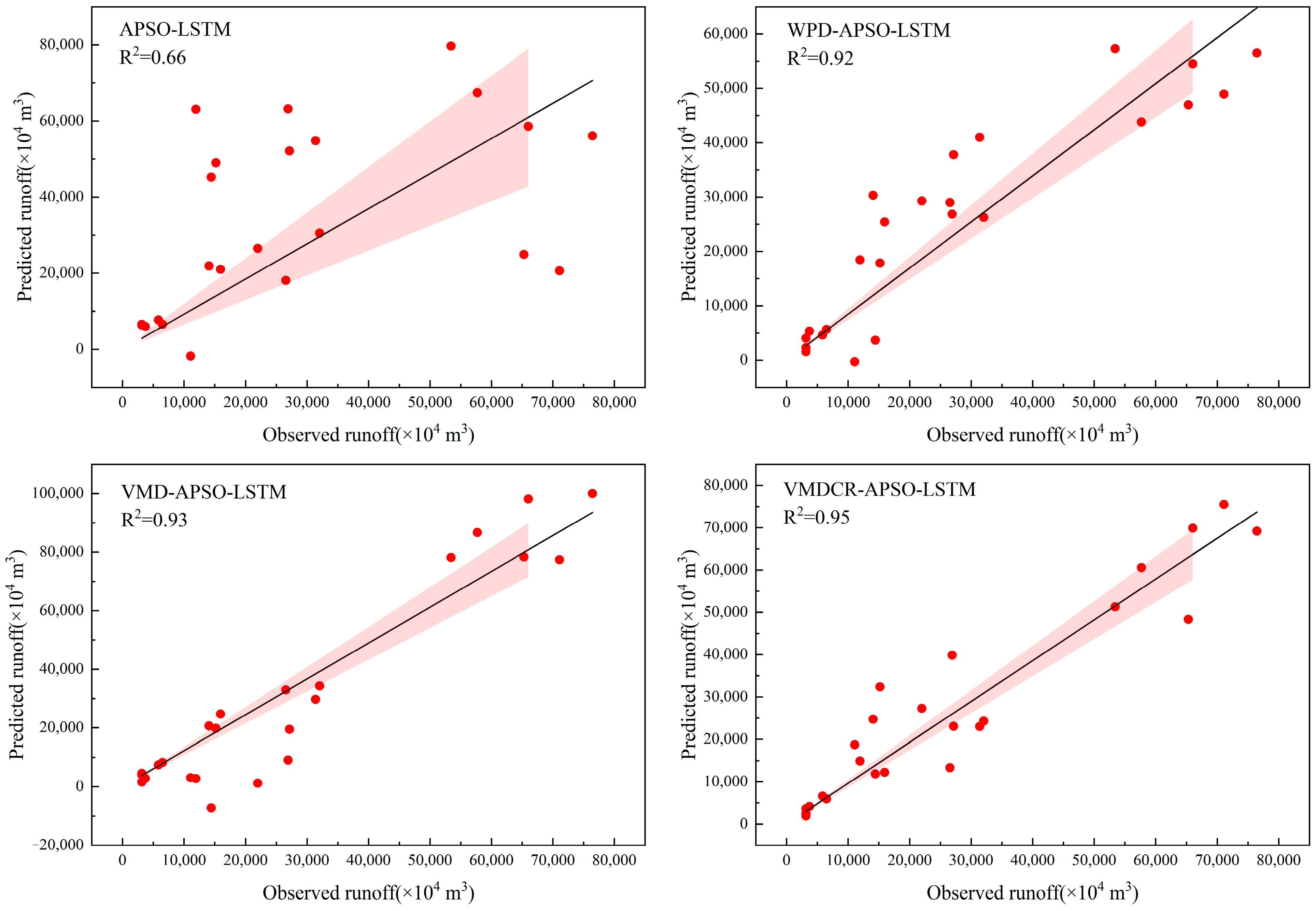
4.4. Prediction Results and Discussion

The prediction results of each model for different hydrological stations are illustrated in Figure 8. From Figure 8, it can be noticed that the S1 (APSO-LSTM) model can basically capture the future trend of runoff, but performs poorly in predicting the runoff variation process. Compared with S1, the S2 (VMD-APSO-LSTM) model has significantly improved the prediction effect on the runoff change process, and can more accurately reflect the trend of the runoff process during the test period. It is indicated that introducing the decomposition method to process the runoff sequences can obtain better linear data, thereby reducing the difficulty of model prediction and improving the prediction accuracy. However, it should be pointed out that, due to the small sample size of the annual runoff series, the endpoint effect of the S2 model results in significant deviations in predicted results for the two ends of the test period, namely, 1995 and 2000, for each station. As for the S3 (WPD-APSO-LSTM) model, although it can also accurately reflect the trend of runoff process changes during the testing period, and the overall prediction results at the boundaries are better than that of S2, it still exhibits significant flaws. For example, the boundary prediction of the Lancun Station in 2000 is negative, as shown in Figure 8b. Comparing the calculation results of the above three models, the S4 (VMDSC-APSO-LSTM) model proposed in this study not only grasps the trend of the runoff process more precisely, but also performs well at the boundaries of the test period, especially at Zhaishang Station, Lancun Station, and Fenhe Reservoir Station, where the forecasting results are completely superior to those of S3.

In order to further clarify the performance of each model at different stations, the fitting effects between the predicted and measured values of the model during the test period at each station are analyzed, and the evaluation indexes of each model are calculated. The results are shown in Figure 9 and

Table 4. Performance indicators of each model.

Station	Indicators	S1	S2	S3	S4
Zhaishang Station	NSE	−0.07	0.39	0.75	0.87
	RMSE	24,948.33	18,887.16	11,962.67	8722.91
	MAE	23,470.33	15,216.65	10,851.92	7229.79
Lancun Station	NSE	−1.49	0.47	0.75	0.90
	RMSE	35,011.80	16,075.52	11,043.59	6905.67
	MAE	30,257.54	14,475.16	8550.40	5891.22
Fenhe Reservoir Station	NSE	0.18	0.49	0.60	0.72
	RMSE	17,748.42	14,024.10	12,402.17	10,481.04
	MAE	12,186.56	11,023.81	11,035.34	9205.33
Shangjingyou Station	NSE	−2.54	-0.01	0.24	0.73
	RMSE	2618.11	1395.83	1212.89	726.03
	MAE	2348.73	1360.30	1167.03	679.19

, respectively. It can be seen from Figure 9 that the S4 model has the highest degree of scatter compactness, with the adjusted R² = 0.95, followed closely by S2, S3, and S1 models, with the corresponding adjusted R² of 0.93, 0.92, and 0.66, respectively. The above results indicate that the S4 model proposed in this article demonstrates the most outstanding performance overall in the annual runoff prediction for the four stations.

A further observation of Table 4 shows that the overall performance of the four models in this study is ranked as S4 > S3 > S2 > S1. Specifically, compared to S3, the S4 model reduces RMSE by 15.49–40.14%, and MAE by 16.58–41.80%. Compared to S2, the S4 model brings down RMSE and MAE by 25.26–57.04% and 16.50–59.30%, respectively. The above results illustrate that the S4 model, which combines VMD and SC algorithms, is more suitable for annual runoff prediction with relatively few runoff samples. It can effectively improve the significant endpoint effect of the S2 model when the length of the annual runoff series is small, and the improved effect is even better than that of the prediction model using S3. In addition, compared with the basic model S1, the reduction in RMSE and MAE of the S4 model are cut down by a greater extent, ranging from 40.95–80.28% and 24.46–80.53%, respectively. It is indicated that the synergistic effect of decomposition, clustering, and the LSTM model can weaken the inadequacy of the individual LSTM model, minimize the complexity of annual runoff series, and ameliorate the forecasting accuracy. Observing the NSE values of each model in Table 4, it is evident that the NSE values of each station based on the S4 model are all greater than 0.70, especially at Zhaishang Station and Lancun Station, with the NSE values of 0.87 and 0.90, respectively. According to the standard for hydrological information and hydrological forecasting [37], the accuracy levels of the four stations predicted by the S4 model have reached level B (good, NSE ≥ 0.70).

In summary, in the prediction of annual runoff, the VMDSC-APSO-LSTM model proposed in this paper outperforms the other comparative models. This can be attributed to several factors: (1) The VMD method can better capture the essential features of the annual runoff series, such as the trend and period, by decomposing the non-stationary annual runoff series with spatial heterogeneity into multiple modal components. (2) Integrating the VMD and SC algorithm enables the recombination of the decomposed modal components, thus minimizing the number of decomposition layers. The reduction in layers decreases the loop iteration of the program, boosting the computational speed of the combined model, which helps mitigate the adverse effects of endpoint effects caused by modal components. It can be seen that a prediction model combining the decomposition method, the clustering method, the heuristic optimization algorithm, and the deep learning technology can achieve a more satisfactory prediction effect in the annual runoff prediction.

5. Conclusions

Based on the characteristics of a small sample size of annual runoff series and a serious endpoint effect during decomposition, starting from the theoretical VMD, and with the aim of suppressing the endpoint effects, an annual runoff prediction model called VMDSC-APSO-LSTM is proposed in this paper, which couples VMD and SC methods on the basis of an improved machine learning algorithm. The model combines two efficient signal-processing methods, VMD and SC. By decomposing and clustering the annual runoff series, it can capture the key feature information of the annual runoff series more accurately and finally improve the prediction accuracy. The proposed model and three comparative models are applied to the annual runoff prediction of four hydrological stations in the upper reaches of Fenhe Basin. The results show that the VMDSC-APSO-LSTM model proposed in this paper is significantly better than other comparative models in terms of accuracy. Based on the model proposed in this paper, the methodological barriers encountered in predicting runoff with limited sample data have been effectively addressed to a certain extent, providing valuable insights for annual runoff prediction and other short-term hydrological element prediction.

References

1. Wang, Y.; Xu, H.; Li, Y.; Liu, L.; Hu, Z.; Xiao, C.; Yang, T. Climate change impacts on runoff in the Fujiang River Basin based on CMIP6 and SWAT model. Water 2022, 14, 3614. [Google Scholar] [CrossRef]
2. Zhang, W.; Furtado, K.; Zhou, T.; Wu, P.; Chen, X. Constraining extreme precipitation projections using past precipitation variability. Nat. Commun. 2022, 13, 6319. [Google Scholar] [CrossRef] [PubMed]
3. Bolorinos, J.; Rajagopal, R.; Ajami, N.K. Do water savings persist? Using survival models to plan for long-term responses to extreme drought. Environ. Res. Lett. 2022, 17, 094032. [Google Scholar] [CrossRef]
4. Taniguchi, K.; Kotone, K.; Shibuo, Y. Simulation-based assessment of inundation risk potential considering the nonstationarity of extreme flood events under climate change. J. Hydrol. 2022, 613, 128434. [Google Scholar] [CrossRef]
5. Cho, K.; Kim, Y. Improving streamflow prediction in the WRF-Hydro model with LSTM networks. J. Hydrol. 2022, 605, 127297. [Google Scholar] [CrossRef]
6. Song, C.M. Data construction methodology for convolution neural network based daily runoff prediction and assessment of its applicability. J. Hydrol. 2022, 605, 127324. [Google Scholar] [CrossRef]
7. Zhao, X.; Lv, H.; Lv, S.; Sang, Y.; Wei, Y.; Zhu, X. Enhancing robustness of monthly streamflow forecasting model using gated recurrent unit based on improved grey wolf optimizer. J. Hydrol. 2021, 601, 126607. [Google Scholar] [CrossRef]
8. Han, D.; Liu, P.; Xie, K.; Li, H.; Xia, Q.; Cheng, Q.; Wang, Y.; Yang, Z.; Zhang, Y.; Xia, J. An attention-based LSTM model for long-term runoff forecasting and factor recognition. Environ. Res. Lett. 2023, 18, 024004. [Google Scholar] [CrossRef]
9. Shi, W.; Wang, N.; Wang, M.; Li, D. Revised runoff curve number for runoff prediction in the Loess Plateau of China. Hydrol. Process. 2021, 35, e14390. [Google Scholar] [CrossRef]
10. Yan, B.; Mu, R.; Guo, J.; Liu, Y.; Tang, J.; Wang, H. Flood risk analysis of reservoirs based on full-series ARIMA model under climate change. J. Hydrol. 2022, 610, 127979. [Google Scholar] [CrossRef]
11. Zhang, J.; Yan, H. A long short-term components neural network model with data augmentation for daily runoff forecasting. J. Hydrol. 2023, 617, 128853. [Google Scholar] [CrossRef]
12. Wang, X.; Wang, Y.; Yuan, P.; Wang, L.; Cheng, D. An adaptive daily runoff forecast model using VMD-LSTM-PSO hybrid approach. Hydrol. Sci. J. 2021, 66, 1488–1502. [Google Scholar] [CrossRef]
13. Li, F.-F.; Cao, H.; Hao, C.-F.; Qiu, J. Daily streamflow forecasting based on flow pattern recognition. Water Resour. Manag. 2021, 35, 4601–4620. [Google Scholar] [CrossRef]
14. Li, Y.; Wang, D.; Wei, J.; Li, B.; Xu, B.; Xu, Y.; Huang, H. A medium and long-term runoff forecast method based on massive meteorological data and machine learning algorithms. Water 2021, 13, 1308. [Google Scholar] [CrossRef]
15. Adaryani, F.R.; Mousavi, S.J.; Jafari, F. Short-term rainfall forecasting using machine learning-based approaches of PSO-SVR, LSTM and CNN. J. Hydrol. 2022, 614, 128463. [Google Scholar] [CrossRef]
16. Wang, Y.; Wang, W.; Xu, D.; Zhao, Y.; Zang, H. A compound approach for ten-day run of prediction by coupling wavelet denoising, attention mechanism, and LSTM based on GPU parallel acceleration technology. Earth Sci. Inform. 2024, 17, 1281–1299. [Google Scholar] [CrossRef]
17. Gauch, M.; Kratzert, F.; Klotz, D.; Nearing, G.; Lin, J.; Hochreiter, S. Rainfall-runoff prediction at multiple timescales with a single Long Short-Term Memory network. Hydrol. Earth Syst. Sci. 2021, 25, 2045–2062. [Google Scholar] [CrossRef]
18. He, X.; Luo, J.; Li, P.; Zuo, G.; Xie, J. A hybrid model based on variational mode decomposition and gradient boosting regression tree for monthly runoff forecasting. Water Resour. Manag. 2020, 34, 865–884. [Google Scholar] [CrossRef]
19. Wang, W.; Wang, B.; Chau, K.W.; Xu, D. Monthly runoff time series interval prediction based on WOA-VMD-LSTM using non-parametric kernel density estimation. Earth Sci. Inform. 2023, 16, 2373–2389. [Google Scholar] [CrossRef]
20. Demir, I.; Xiang, Z.; Demiray, B.; Sit, M. WaterBench-Iowa: A large-scale benchmark dataset for data-driven streamflow forecasting. Earth Syst. Sci. Data 2022, 14, 5605–5616. [Google Scholar] [CrossRef]
21. Liu, W.; Cao, S.; Chen, Y. Applications of variational mode decomposition in seismic time-frequency analysis. Geophysics 2016, 81, V365–V378. [Google Scholar] [CrossRef]
22. Xu, Z.; Mo, L.; Zhou, J.; Fang, W.; Qin, H. Stepwise decomposition-integration-prediction framework for runoff forecasting considering boundary correction. Sci. Total Environ. 2022, 851, 158342. [Google Scholar] [CrossRef] [PubMed]
23. Chen, S.; Ren, M.; Sun, W. Combining two-stage decomposition based machine learning methods for annual runoff forecasting. J. Hydrol. 2021, 603, 126945. [Google Scholar] [CrossRef]
24. Shahram, H.; Hossein, Z.; Andrea, C.; Saeid, L. Offshore wind power forecasting based on WPD and optimised deep learning methods. Renew. Energy 2023, 218, 119241. [Google Scholar]
25. Wei, H.; Wang, Y.; Liu, J.; Cao, Y. Monthly Runoff Prediction by Combined Models Based on Secondary Decomposition at the Wulong Hydrological Station in the Yangtze River Basin. Water 2023, 15, 3717. [Google Scholar] [CrossRef]
26. Dragomiretskiy, K.; Zosso, D. Variational mode decomposition. IEEE Trans. Signal Process. 2014, 62, 531–544. [Google Scholar] [CrossRef]
27. Abdoos, A.A. A new intelligent method based on combination of VMD and ELM for short term wind power forecasting. Neurocomputing 2016, 203, 111–120. [Google Scholar] [CrossRef]
28. Von Luxburg, U. A tutorial on spectral clustering. Stat. Comput. 2007, 17, 395–416. [Google Scholar] [CrossRef]
29. Qiao, G.; Yang, M.; Zeng, X. Monthly-scale runoff forecast model based on PSO-SVR. J. Phys. Conf. Ser. 2022, 2189, 012016. [Google Scholar] [CrossRef]
30. Gobashy, M.; Abdelazeem, M. Metaheuristics inversion of self-potential anomalies. In Self-Potential Method: Theoretical Modeling and Applications in Geosciences; Springer: Cham, Switzerland, 2021; pp. 35–103. [Google Scholar]
31. Tamilmani, G.; Varma, C.P.; Devi, V.B.; Babu, G.R. Medical image segmentation using grey wolf-based u-net with bi-directional convolutional LSTM. Int. J. Pattern Recognit. Artif. Intell. 2024, 38, 2354025. [Google Scholar] [CrossRef]
32. Fakhar, M.S.; Kashif, S.A.R.; Liaquat, S.; Rasool, A.; Padmanaban, S.; Iqbal, M.A.; Baig, M.A.; Khan, B. Implementation of APSO and improved APSO on non-cascaded and cascaded short term hydrothermal scheduling. IEEE Access 2021, 9, 77784–77797. [Google Scholar] [CrossRef]
33. Wen, L.; Song, Q. ELCC-based capacity value estimation of combined wind-storage system using IPSO algorithm. Energy 2023, 263, 125784. [Google Scholar] [CrossRef]
34. Fang, W.; Huang, S.; Ren, K.; Huang, Q.; Huang, G.; Cheng, G.; Li, K. Examining the applicability of different sampling techniques in the development of decomposition-based streamflow forecasting models. J. Hydrol. 2019, 568, 534–550. [Google Scholar] [CrossRef]
35. Hao, Y.; Lu, J.; Peng, G.; Wang, M.; Li, J.; Wei, G. F10.7 Daily forecast using LSTM combined with VMD method. Space Weather 2024, 22, e2023SW003552. [Google Scholar] [CrossRef]
36. Gendeel, M.; Yuxian, Z.; Aoqi, H. Performance comparison of ANNs model with VMD for short-term wind speed forecasting. IET Renew. Power Gener. 2018, 12, 1424–1430. [Google Scholar] [CrossRef]
37. GB/T22482-2008; Ministry of Water Resources. Hydrology Information Forecast Specification. China Standards Press: Beijing, China, 2009. (In Chinese)
Figure 1. The internal operation structure of LSTM.
Water 16 01179 g001
Figure 2. Operation flow chart of APSO-LSTM model.
Water 16 01179 g002
Figure 3. Structure framework diagram of VMDSC-APSO-LSTM model.
Water 16 01179 g003
Figure 4. Location of study area and hydrological stations.
Water 16 01179 g004
Figure 5. The results of center frequencies for each IMF at different decomposition layers.
Water 16 01179 g005
Figure 6. Results of the variational mode decomposition at each station.
Water 16 01179 g006
Figure 7. Clustering results of IMFs.
Water 16 01179 g007
Figure 8. Annual runoff prediction results for each station.
Water 16 01179 g008
Figure 9. Scatter plot for prediction results of each model.
Water 16 01179 g009