
Stability Analysis of Cofferdam with Double-Wall Steel Sheet Piles under Wave Action from Storm Surges
by
 , ,
, ,
Yan Zhu
1,
Jingchao Bi
1,
Haofeng Xing
2,3,*,
Ming Peng
2,3,
Yu Huang
2,3,
Kaifang Wang
1 and
Xinyu Pan
1 1
Shanghai Research Center of Ocean and Shipbuilding Engineering, China Shipbuilding NDRI Engineering Co., Ltd., Shanghai 200090, China
2
Key Laboratory of Geotechnical and Underground Engineering of Ministry of Education, Department of Geotechnical Engineering, Tongji University, Shanghai 200092, China
3
Department of Geotechnical Engineering, College of Civil Engineering, Tongji University, Shanghai 200092, China
*
Author to whom correspondence should be addressed.
Water 2024, 16(8), 1181; https://doi.org/10.3390/w16081181
Submission received: 26 March 2024
/
Revised: 14 April 2024
/
Accepted: 17 April 2024
/
Published: 20 April 2024
(This article belongs to the Special Issue Wave–Structure Interaction in Coastal and Ocean Engineering)
Abstract
:Double-wall steel sheet piles (DSSPs) are widely used in large-span cofferdams for docks due to their good performance against wave action during storm surges. This paper describes a study of the dynamic behavior of a DSSP cofferdam under wave action through flume tests and a numerical simulation that combined computational fluid dynamics (CFD) and the finite element method. The influences of the water level and wave height on the DSSP cofferdam were investigated experimentally and numerically. Tall waves in shallow water broke upon and impacted the seaside pile with large dynamic wave pressure, dramatically increasing the stress and displacement of the seaside pile. The overlap of the traveling and reflected waves increased the excess pore water pressure near the seaside pile due to taller overlapped waves and higher wave frequency. The DSSP cofferdam failed under the combined actions of the dynamic wave pressure and erosion of the landside seabed. The leakage and overflow of the breaking waves resulted in significant erosion of the landside seabed and greatly weakened the support of the seabed. The dynamic wave pressure then pushed the DSSP cofferdam until it failed. The simulation with the combined methods of CFD and FEM resulted in trends that were similar to those of the test measurements. Compared to the quasi-static method and pseudo-dynamic method, the results of the simulation via the present method were much closer to the test results because the simulation included the effects of breaking waves. The reinforced measure worked well to prevent the DSSP cofferdam in a sandy seabed foundation from continuous failures of deformation–leakage–erosion–tilting. However, it failed in a clay interlayer seabed foundation due to the large settlement.
1. Introduction
Storm surge, which is one of the most destructive coastal hazards, incurs the most human life and property losses in coastal zones (Gonnert and Gerkensmeier [1]; Wahl et al. [2]; Streicher et al. [3]; Toyoda et al. [4]). Double-wall steel sheet piles (DSSPs), composed of two rows of steel sheet piles separated by soil infill and connected by steel tie rods, are widely used as retaining structures to protect large-span cofferdams for docks from water and waves (Gui and Han [5]). DSSPs have good performance against wave action during storm surges. For instance, during the 2011 Tohoku earthquake tsunami, the coastal embankments in Fukushima, Japan were severely damaged and even completely flooded in many areas. Surprisingly, a segment of the cofferdam made with DSSPs remained stable overall (Furuichi et al. [6]). The cofferdam did not bend or tilt obviously. Only erosion of the sand infill between the two rows of piles was observed. This case raises questions about the DSSP: Why did the DSSP withstand such a very large dynamic load? How did the components of the DSSP, namely, steel sheet piles, soil infill, and steel tie rods, behave during the wave action? What would the failure mode have been if the waves had occurred at a higher water level and been taller during the storm surge?
There are many more available studies on single-wall steel sheet piles (SSSPs) than DSSPs (Cheng et al. [7]; Wang et al. [8]; Yi et al. [9]). Kimura et al. [10] developed an H-joint steel pipe sheet pile technology and examined this technology through field construction tests, full-scale bending tests, and centrifuge tests. Mawer and Byfield [11] investigated the reduced modulus action in a U-section steel sheet pile retaining wall through experimental tests with miniature piles and numerical simulations of full-scale piles. Inazumi et al. [12] evaluated the water cut-off performance of H-jointed steel pipe sheet piles with H-H joints that were attached to water-swellable materials under various conditions. Wang et al. [13] used 3-D finite element method (FEM) techniques to investigate the reduced modulus action in a case study of a foundation pit supported by U-section steel sheet piles in the Yangtze River. Osthoff and Grabe [14] presented a method to simulate the penetration of steel sheet piles while considering the deformation behavior of slender profiles with relatively low bending and torsional stiffness using the coupled Euler–Lagrange (CEL) approach. Kang et al. [15] experimentally and numerically studied a vertical truncated dumbbell-shaped cylinder in a cofferdam for a bridge by comparing only wave–wave interactions vs. wave–wave and wave–current interactions. Despite some relevant information in the SSSP studies in the above literature, more detailed efforts are necessary to study DSSPs since the differences between DSSPs and SSSPs are very large.
In exploring double-wall sheet steel piling (DSSP) structures, notable contributions span from Ohori et al. [16], with their statistical model for double-wall sheet pile constructions, to more recent examinations of their dynamic behaviors under various environmental conditions. Khan et al. [17] delved into the performance of double-wall sheet pile cofferdams on clay through centrifuge model testing. A significant onsite evaluation was carried out by Hou et al. [18] at a major dock project in Shanghai, assessing the deformation characteristics of a large-span DSSP cofferdam. Investigations into DSSP efficacy against tsunami impacts were undertaken by Furuichi et al. [6] and Mitobe et al. [19], who demonstrated superior resistance of double-walled configurations in flume tests. Zhu et al. [20] applied the Bayesian approach to enhance the reliability assessment of DSSPs, integrating both statistical and field data effectively. The innovative combination of perpendicular partition and double-wall sheet piles for levee reinforcement was analyzed by Fujiwara et al. [21] through shaking table experiments and 2-D simulations, assessing earthquake response. Xue et al. [22] conducted stability analysis for cofferdams of pile wall frame structures by engineering tests and 3-D FEM numerical simulations and proposed a design method based on the limit equilibrium method. Despite widespread application, the detailed mechanical behaviors and failure mechanisms of DSSPs, particularly under storm surge conditions, have remained underexplored.
This study introduces a hybrid approach combining experimental and computational models to dissect the dynamic responses of DSSPs to wave actions. Initial phases focused on designing and configuring experimental setups, including model cofferdams and testing protocols. Subsequent analyses covered seabed erosion, structural deformations, and failures, with numerical simulations providing deeper insights into the DSSPs’ behavior during wave interactions, corroborated by experimental findings. The outcome offers fresh perspectives on DSSP performance and their protective efficacy against wave-induced forces.
2. Experimental Details
2.1. Test Apparatus
The model test was performed in the wave flume system at Tongji University, as shown in Figure 1. The length, width, and depth of the flume were 42 m, 0.8 m, and 1.25 m, respectively. The gradient of the flume bottom was zero. The bottom, head, and tail of the flume were concrete structures, and the middle section was a steel structure with transparent glass on both sides for making observations. The wave-generating system was located at the head of the wave flume, as shown in Figure 1b. Water waves were generated by pushing the steel board (Figure 1c) back and forth. The wave generator could simulate regular waves, elliptical cosine waves, solitary waves, and superimposed breaking waves. The range for wave heights was 0.02–0.3 m. The generated wave period was in the range of 0.5–5 s. The wave-generating machine, manufactured by Siemens in Munich, Germany, was controlled by a dual-core 2.6 GHz compatible computer (Figure 1d). The wave height was monitored and validated by a wave height sensor and data collection system (Figure 1d). Vertical energy dissipation nets were arranged at both sides of the flume to reduce the reflection effect.
2.2. Test Model and Materials
The test was modeled after the cofferdam at the Changxing dock, as shown Figure 2. The cofferdam was built with double rows of steel sheet piles on both sides. The height of the steel sheet pile was 18 m, which was 9 m above the seabed. The two rows of piles were connected with steel tie rods on the top, and the space between the two rows of piles was filled with medium-coarse sand to maintain the entire structure.
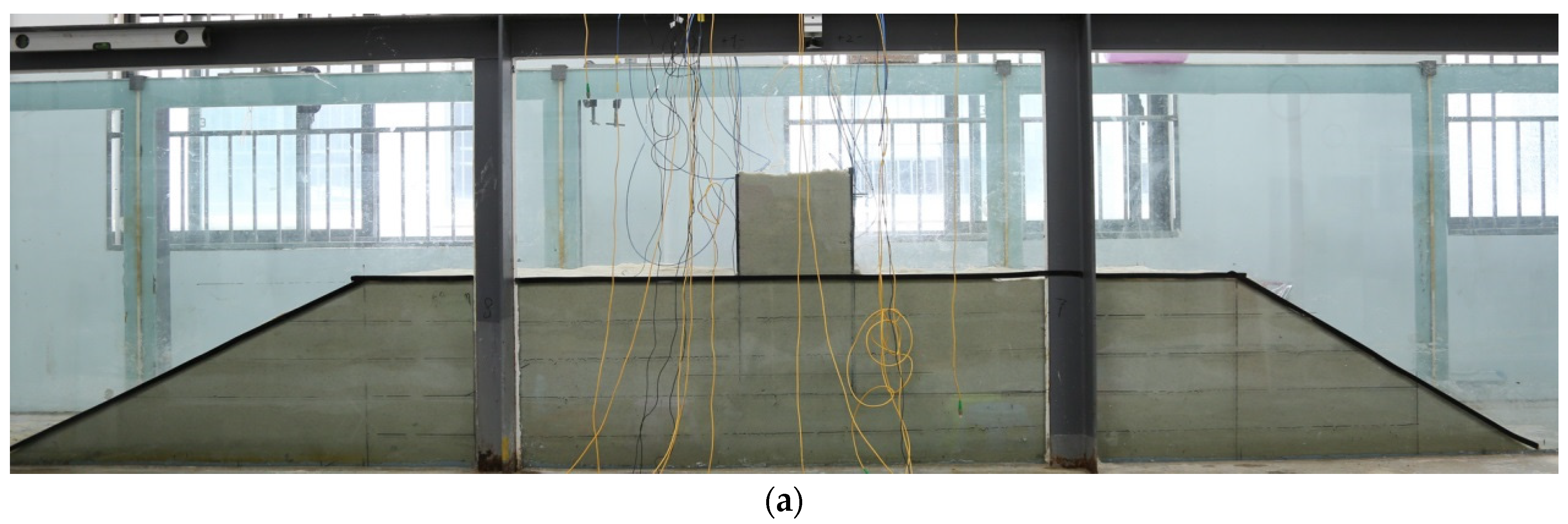
The model cofferdam was built with a geometric similarity ratio of 1:30, as shown in Figure 3 and Figure 4. The similarity ratios of time and density were 1:5.48 and 1:1, respectively. The other similarity ratios can be derived accordingly. The seabed was in the shape of a trapezoid with a height of 50 cm, top width of 230 cm, and a bottom width of 403.2 cm. Positioned centrally on this seabed, the model featured two rows of steel sheet piles, each 60 cm high, surpassing the seabed by 30 cm. These rows were bridged by four steel tie rods spaced 22 cm apart, with pile thickness and tie rod diameter set at 1.5 mm and 5.2 mm, aligning with the established similarity ratio. The inter-pile space and seabed utilized 0.35 mm quartz sand as fill material, with sand properties detailed in Table 1.
2.3. Monitoring System and Construction of the Model Cofferdam
The layout of the monitors is shown in Figure 3. Ten pressure gauges, manufactured by Nanzee Sensing in Suzhou, China, (quasi-distributed fiber FBG, demodulator sampling frequency 2000 Hz) were set to monitor the horizontal earth pressure close to the piles, with six inside and four outside the cofferdam. Six piezometers, manufactured by Nanzee Sensing in Suzhou, China, (KPE-200KPB, the measuring range is 200 kPa, sampling frequency 100 kHz) were set to monitor the water pressure beneath the seabed. Ten optical fiber strain gauges were set on the offshore sides of both piles to monitor the stress of the piles. Four high-speed cameras were set with side view, top view, front view (landside), and back view (offshore side).
The cofferdam model was built with the following steps:
- (1)
- The seabed and cofferdam outline were marked on a glass wall, followed by the layered construction of the seabed using quartz sand, each layer 10 cm thick. Piezometers were buried in the seabed according to the locations shown in Figure 3.
- (2)
- The two rows of steel sheet piles were installed with soil pressure sensors and optic fiber sensors (see Figure 3b) in the reserved notch, ensuring a depth inside the seabed of 30 cm. Two U-shaped rubber sealing strips were installed between the piles and the glass wall to prevent boundary seepage.
- (3)
- Four steel tie rods connecting two rows of steel sheet piles were installed (see Figure 3c). The optic fiber stress sensors were set on the middle of two tie rods to measure the tensile stress.
- (4)
- The space between the two rows of steel sheet piles was filled with quartz sand of the designed density until the cofferdam height reached 60 cm.
- (5)
- Five high-speed cameras were installed with full side view (the full seabed), local side view (the full cofferdam), top view, offshore side view, and landside view. The monitoring equipment was commissioned.
2.4. Test Procedure
- (1)
- The offshore side was filled to water depth (D) of 65 cm in 15 min followed by waiting for 30 min until the seepage flow reached a steady state with a steady phreatic line.
- (2)
- A sine wave was generated with wave height (HW) of 4 cm and period of 2 s for 15 min. Then, the wave-generating machine was turned off for 2–5 min until the water level basically became steady. This stage was called Stage 1.
- (3)
- Water was added to keep D of 65 cm and replace water lost due to seepage and wave overflow. A sine wave was generated with HW of 8 cm and period of 2 s for 12.5 min. Then, the wave-generating machine was turned off for 2–5 min until the water level basically became steady. This stage was called Stage 2.
- (4)
- Water was added to keep D at 65 cm. A sine wave with HW of 12 cm and period of 2 s was generated for 10 min. Then, the wave-generating machine was turned off for 7 min until the water level basically became steady. This stage was called Stage 3.
- (5)
- Water was added to the offshore side with D of 73 cm in 6 min followed by waiting for 1–2 min until the water level became steady. A sine wave was generated with HW of 4 cm and the period of 2 s in 10 min. Then, the wave-generating machine was turned off for 2–5 min until the water level basically became steady. This stage was called Stage 4.
- (6)
- Water was added to maintain a D of 73 cm. Water waves with HW of 8 cm and period of 2 s were generated until the cofferdam failed. This stage was called Stage 5.
3. Test Results and Analysis
3.1. Stage 0 (before the Wave-Generating Stage, D = 0~65 cm)
The moment of starting to add water was set as time 0 s. Water infiltrated the seabed from the upstream slope, and the phreatic line in the seabed rose accordingly. Upon the water level surpassing the seabed’s apex, infiltration ensued atop the seabed, accelerating as it converged with the pre-existing phreatic line originating from the upstream slope, thereby intensifying the rate of seepage (refer to Figure 6 at 11′06″). The pace of seepage decelerated once the phreatic line ascended to the base of the seaside pile. It took more than 8 min for the phreatic line to arrive at the toe of the landside slope. The phreatic line rose steadily, and water seeped out of the downstream slope.
Shortly after the phreatic line reached the landside slope, local sliding occurred. The sliding moved upward along the slope with the continuous rising of the phreatic line (see 18′04″ in Figure 5), making the downstream slope gentler. Combined with the deposition at the adjacent downstream area of the slope toe, a new stable downstream slope with an angle of 15° formed (see 43′33″ in Figure 6), which was much smaller than the original slope angle of 30°. The loss of soil was mainly caused by three factors: the weakening of the shear strength due to saturation, seepage force, and gravitational force.
Figure 7 shows the stresses on both sheet piles (OP1–OP5 and LP1–LP5) and the two middle tie rods (PR1–PR2) measured by the optic fiber sensors and the pore water pressure (P1–P4). In the figure, ‘+’ represents tensile stress and ‘−’ represents compressive stress. The stresses of OP2, OP3, and OP4 decreased at Point A when water arrived at the seabed. The infiltration from the seabed caused the pore water pressure to increase rapidly (Figure 7d), leading to decrease in the stresses of OP2, OP3, and OP4. However, OP1 and OP5 did not change much because they were not in the area influenced by water pressure. The stresses on the landside pile did not change much because the sand infill between the two piles supported the major forces. The stresses on the tie rods decreased slightly after Point A because of the deformation of the seaside pile.
The pore water pressures in the first 10 min were zero since the seepage from the upstream slope of the seabed was rather slow. P1, P2, and P3 increased rapidly after water arrived at the seabed because of the shorter seepage path from the top of the seabed close to the seaside pile. The pore water pressures became steady when the water level reached 65 cm. P3 was the largest since it was located lower than the other two. P4 started to rise at 23 min since it was located at the landside, which indicated that the DSSP was waterproof.
3.2. Stage 1 (D = 65 cm, HW = 4 cm)
Stage 1 with a water level of 65 cm and wave height of 4 cm started at 47′16″ (Figure 8). The wave did not break due to a relatively large water depth of 15 cm. The seabed exhibited fluctuations on the offshore side, which slowly moved toward the cofferdam. Overtopping occurred casually on the top of the cofferdam due to the overlapping of the traveling and reflecting waves, incurring a small groove on the top of the cofferdam near the offshore side pile. The slope on the landside underwent gradual erosion and local sliding due to the dynamic wave that caused the phreatic line to rise (see 55′20″ in Figure 8b). Stage 1 ended at 61′45″. Generally, the wave in Stage 1 did not cause an obvious impact on either the cofferdam or the foundation.
Under the action of the dynamic water pressure, the stress of OP5 in the seaside pile decreased rapidly, as shown in Figure 7a. The stress of OP4 decreased slightly, but the stress of OP3 increased, which denoted the inflection point of the seaside pile located between OP3 and OP4. The stress of the landside pile did not change obviously, except at LP3. Point LP3, which was located closest to the seabed (3 cm above), supported the largest force compared to the other four points, as shown in Figure 7b. The stress of the tie rods decreased sharply after 50 min because the landward deformation of the pile decreased the pre-tension (Figure 7c).
The wave incurred a rise in the pore water pressure in P1, P3, and P4 (Figure 7d), which was much larger than the static pore water pressure, indicating excess pore water pressure. Despite the same heights of P1 and P2, the excess pore water pressure in P1 was much larger than that in P2. The reason was that P1 was much closer to the pile, where the wave frequency is much larger due to the overlap of the traveling and reflected waves.
3.3. Stage 2 (D = 65 cm, HW = 8 cm)
Stage 2 (water level of 65 cm and wave height of 8 cm) started at 63′. The higher wave moved the seabed soils forward and gradually formed a gentle slope. The elevation of the seabed adjacent to the pile rose, making the waves climb higher with larger overtopping volume. In addition, the suction caused by the reflected wave produced a pit beneath the pile (see 68′25″ in Figure 9). The pit decreased due to the continuing transportation of sand from the seaside. A bulge formed 10 cm from the pile, making the water depth here (i.e., 9 cm) much shallower. The wave broke in the shallow water region and caused large dynamic pressure toward the steel sheet pile, deforming the pile periodically toward the landside. The overtopping wave became larger and enlarged the groove on the top of the cofferdam. Moreover, the overtopping wave reached and eroded the landside seabed, forming a trench inside it. The erosion and the rising of the phreatic line made the downstream slope slide at the shoulder (see 73′08″ in Figure 9).
The stresses of OP1 and OP5 in the seaside pile decreased from the start of Stage 2 (Point C) due to the lasting deformation caused by the larger wave (Figure 7a). The stresses of OP2, OP3, and OP4 underwent two phases: fluctuating phase (from Point C to Point D, or from 63 min to 68 min) and rapidly increasing phase (from Point D to Point E, or from 68 min to 78 min). In the first phase, the seabed near the seaside pile was generally flat, and the water was deep enough to make the wave become a standing wave (as shown in Figure 7a,b). However, after Point D (68 min), the deposition close to the pile made the water much shallower. Thus, the wave became a breaking wave instead of a standing wave. The dynamic wave pressure was much larger than that before Point D, leading to larger deformation and stress of the pile.
The large deformation of the seaside pile transformed the force to the landside pile through two paths: the sand infill and the tie rods. The force from the tie rods increased the stresses in LP1 and LP2, while the force from the sand infill decreased the stresses on LP3, LP4, and LP5 (Figure 7b). The stresses in the tie rods fluctuated between Points C and D but increased between Points D and E due to the larger breaking wave action (Figure 7c), similar to those in OP3, OP4, and OP5 in the seaside pile.
The larger wave in Stage 2 increased the pore water pressure and surpassed the largest value in Stage 1 (Figure 7d). The pore water pressures in P1, P2, and P3 showed two peaks in the two phases. The pore water pressure in the second phase was even larger, indicating that the excessive pore water pressure was produced not only by the periodic water pressure but also by the dynamic wave pressure, especially the breaking wave. The water pressure in P4 was not significantly influenced by the breaking wave due to the waterproof DSSP (Points D and E in Figure 7d).
3.4. Stage 3 (D = 65 cm, HW = 12 cm)
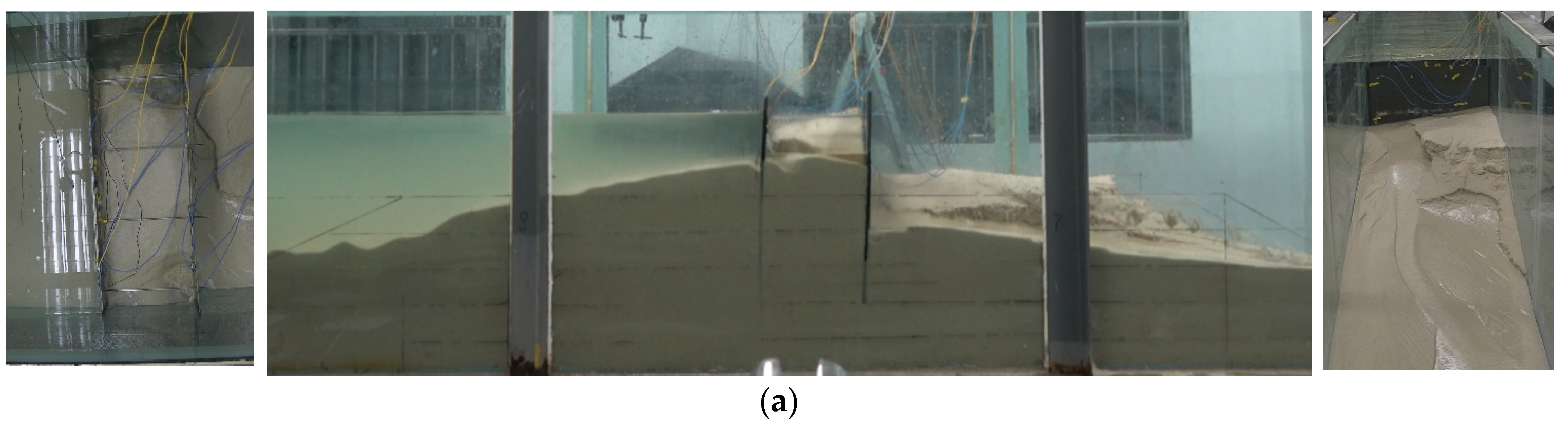
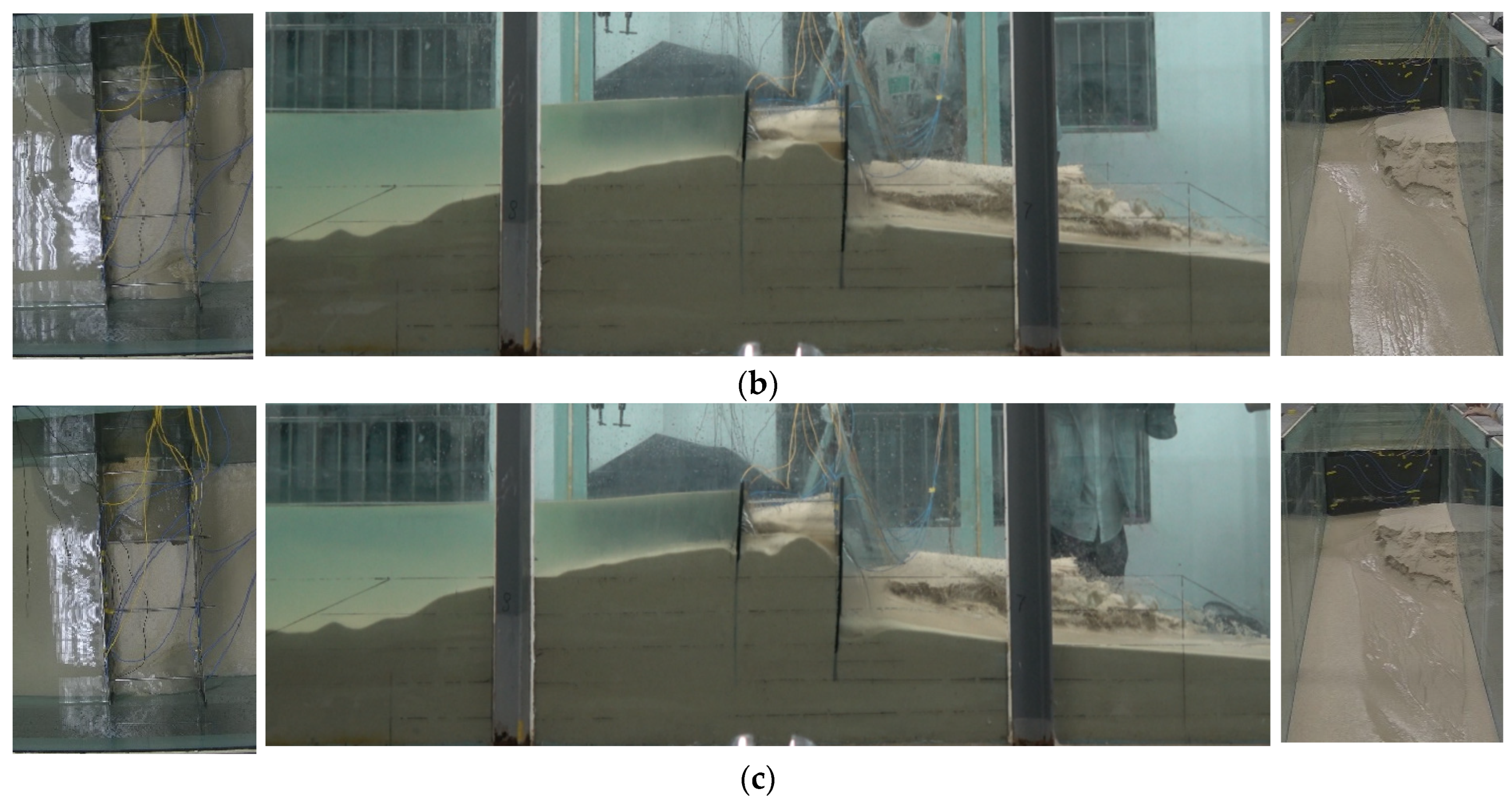
Stage 3 (water level of 65 cm and wave height of 12 cm) started at 77′25″. The highly energetic wave caused more serious erosion on the seabed on the offshore side and deposition on the seabed adjacent to the pile (see Figure 10a,b). A stable slope formed on the offshore side of the seabed with a maximal elevation of 60 cm adjacent to the pile, making the water level rather shallow at 5 cm (see Figure 10c). The dynamic pressure caused by the breaking wave was weakened by the friction action between the water wave and the seabed slope.
The overflow in Stage 3 was very large, making a puddle on the top of the cofferdam. The deformation of the steel sheet pile toward the landside resulted in cracks between the piles and the glass walls on both sides. Water leaked through the cracks and eroded the landside seabed. The leakage of water increased, and the sand between the two piles was washed out, forming a pit with a maximal depth of 17 cm adjacent to the landside pile. The continuing leakage of water eroded the seabed into a gentle slope with an angle of 10°.
The 12 cm high breaking wave made the stresses in OP2, OP3, and OP4 increase significantly (Points E and F in Figure 7a). The stress at OP5 slightly decreased due to the restriction of the soil, especially the increase in the soil thickness due to deposition, which indicated that an inflection point was located between OP4 and OP5.
The erosion of the landside seabed (Figure 10b) largely increased the landward deformation of the landside pile. However, the seaside pile constrained the deformation through the tie rods. In this case, the stress at LP4 increased, but the stresses at LP1 and LP2 decreased. The stress at LP3 did not change obviously, indicating that the erosion of the landside seabed made the reflection point move to the position adjacent to LP3. The stresses in the tie rods (PR1 and PR2) fluctuated and slightly increased due to the complex interaction between the two rows of piles. In addition, the erosion of the sand infill between the two rows of piles made the stresses in PR1 and PR2 asymmetrical (Figure 7c).
The pore water pressure increased at the start of Stage 3 (Point E in Figure 7d) due to the action of the breaking wave and then decreased gradually due to dissipation of the pore water pressure. The pore water pressure of P1 decreased at the fastest rate because of the reduction in the water level due to wave overflow and leakage.
3.5. Stage 4 (D = 73 cm, HW = 4 cm)
The water level increased to 73 cm in Stage 4. The wave with a height of 4 cm was produced at 100′00′’. The wave action had no impact on the offshore side seabed and the deformation of the two steel sheet piles. The wave leakage eroded the sand between the two piles and widened and deepened the trench on the landside. The cofferdam deformed gradually toward the landside during the erosion of soil on the landside (Figure 11).
The pore water pressure before wave generation (the period between Points F and G in Figure 7) was less than that in the former stages because of water lost due to overflow and leakage. Water was supplemented to the level of 73 cm, and the wave with a 4 cm height was generated. The pore water pressure at P1, P2, and P3 increased with the water level and fluctuated during wave action. However, the water pressure at P4 did not change because of the steady water level in the landside seabed caused by overflow and leakage.
3.6. Stage 5 (D = 73 cm, HW = 8 cm)
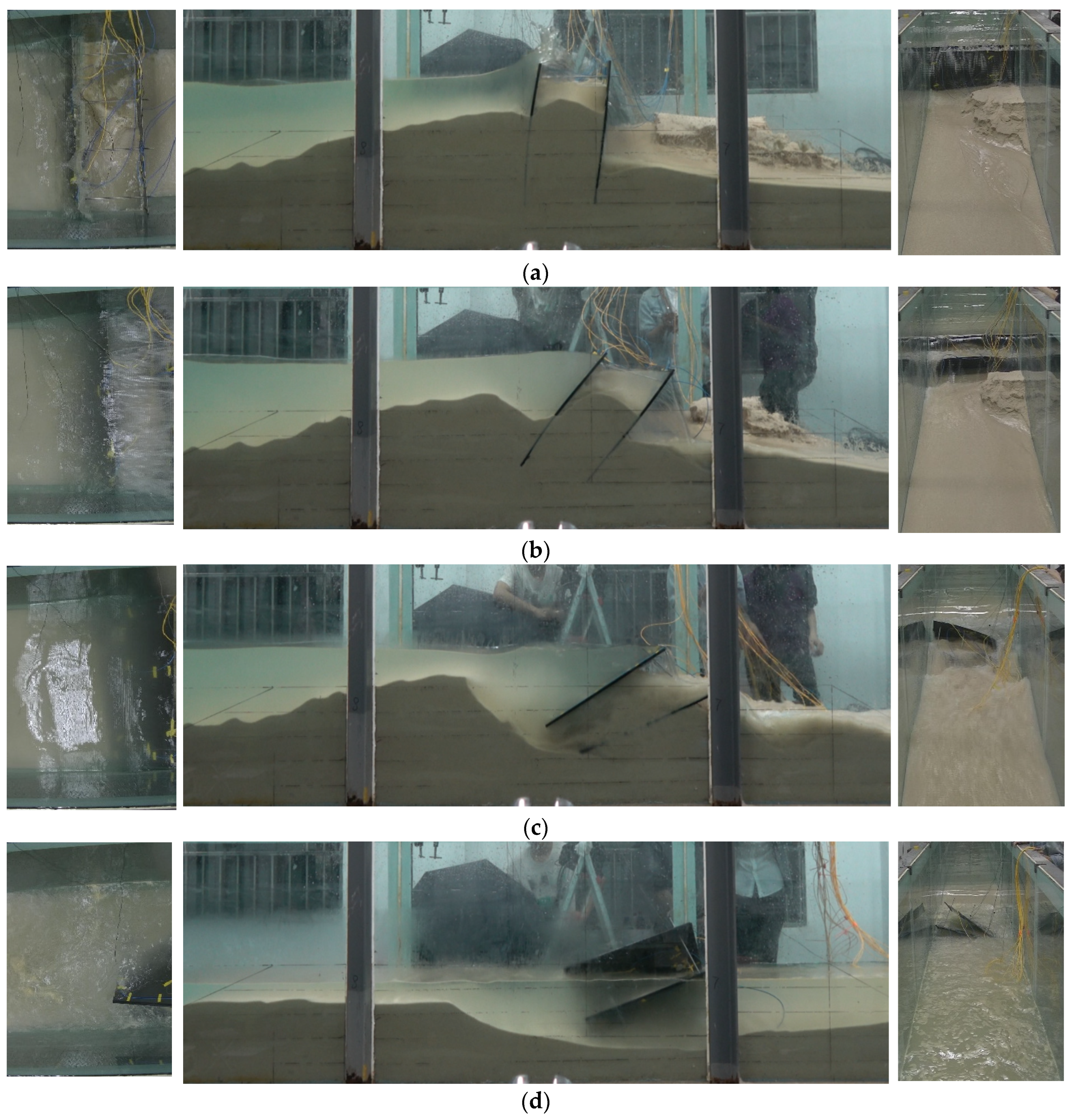
Stage 5 started at 114′45″ when the wave height increased to 8 cm. The dynamic wave pressure pushed the cofferdam to deform significantly (see 115′03″ in Figure 12). The deformation was mainly due to the continuing action of wave pressure and erosion of sand at the toe of the landside pile. The cofferdam tilted and rotated, causing more water to overflow the crest and leak through the gap between the piles and the glass wall (see 115′58″ in Figure 12). The tilting of the offshore side pile caused the formation of an adjacent pit and obvious erosion. The erosion then washed out the foot of the piles.
Despite the failure of the cofferdam, as shown at 115′58″ in Figure 12, the seabed on the offshore side maintained a height of 53 cm. The residual sand on the landside supported the steel sheet pile structure and maintained a water level of 65 cm, which showed that the DSSP could significantly delay the failure of the cofferdam and provide more time for warning and evacuation. The sand beneath the pile structure was then washed away, and the pile structure fell down. After that, the seabed on the offshore side was completely eroded.
The DSSP cofferdam failed soon after an 8 cm high wave was generated, and the stresses in the two rows of piles and the tie rods and the pore water pressure underwent very large fluctuations and decreased to zero until the structure completely failed (Figure 7). It should be noted that structural failures in cofferdams, such as cracks, breaks, and significant deformations caused by material fatigue and overload, as well as substantial deformations due to foundation settlement or slippage, are all considered critical failure points of the cofferdam structure. Moreover, if the sealing system of a cofferdam fails to effectively prevent water leakage, regardless of the absence of overt physical deformations, it is considered a functional failure of the cofferdam.
3.7. Deformation during Failure of the DSSP Cofferdam
Figure 13 shows the deformation of the DSSP cofferdam and seabed during failure. The seaside seabed underwent erosion in the seaward half and deposition in the landward half, as shown in the left part of Figure 13. In particular, deposition close to the seaside pile made the wave break with large dynamic pressure. The sand infill was eroded due to the large leakage through the gap between the pile and glass wall, which resulted from deformation caused by the impact of waves. The soil in the landside seabed was eroded first by leakage when the water level was smaller (65 mm) and then by overflow when the water level (73 cm) and wave height (8 mm) were larger.
The deformation of the DSSP structure was highly dependent on the erosion of the soil in the landside seabed and the sand infill between the two piles [23]. The erosion of the sand infill made the seaside pile deform in the landward direction and greatly reduced the constraints of the tie rods between the two piles. Moreover, the soil erosion in the landside seabed reduced the insertion depth and tilted the landside pile. Therefore, the DSSP cofferdam underwent a cascading failure of ‘deformation–leakage–landside soil erosion–landside pile tilt–more overflow erosion–collapse’.
4. Numerical Simulation of the Dynamic Behavior of the DSSP in the Presence of Waves
4.1. Methodology
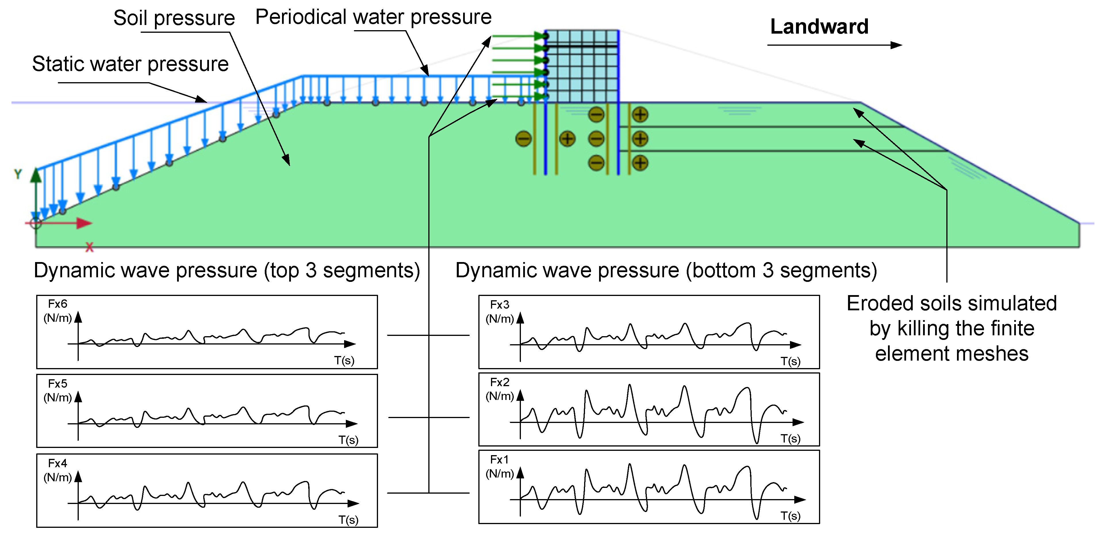
The dynamic behavior of the DSSP cofferdam in the presence of waves was simulated by the combination of computational fluid dynamics (Simulia Xflow, or Xflow for short, version2020) and finite element software (Plaxis Dynamic, version2020), as shown in Figure 14a. The forces on a DSSP cofferdam in the coastal zone are shown in Figure 14b. The offshore side of the cofferdam was subjected to earth pressure, periodic static water pressure, and dynamic wave pressure, and the landside of the cofferdam was subjected to earth pressure and hydrostatic pressure. The hydraulic and hydrodynamic parameters (i.e., periodic static water pressure and dynamic wave pressure), which were obtained by simulating the wave generation, traveling, and action on the steel sheet pile via Simulia Xflow, were extracted and applied in the Plaxis Dynamic software to simulate the dynamic behavior of the cofferdam. Soil erosion was simulated by removing the corresponding finite element mesh in the cofferdam model.
4.1.1. Introduction to Simulia Xflow
Xflow is computational fluid dynamics software developed by Dassault Systèmes. Lattice Boltzmann methods are embedded in Xflow using particle-based Lagrangian methods. The lattice Boltzmann method is used to solve Boltzmann’s transport equation using probability distribution functions to describe fluid flow on the mesoscopic scale (Boltzmann [24]). The continuous Boltzmann equation is discretized into a velocity model, and the equilibrium distribution function is determined by combining the equation derived from the constraints. The macroscopic mass and macroscopic velocity can be obtained from the mass density equation and the momentum density equation.
4.1.2. Introduction to Plaxis Software
Plaxis is general geotechnical finite element calculation software developed by Delft University of Technology in the Netherlands in 1987. Plaxis was formally established in 1993 and acquired by Bentley after 2018. Thus far, it has professional modules such as Plaxflow (seepage module), Dynamics (power module), Monoto (large-diameter single pile), and so on. The dynamic calculations in this section were mainly carried out in Plaxis Dynamics.
4.1.3. Wave Functions in the Five Tests
Based on the above basic assumptions and the wave theory of linear waves (Figure 15), the wave surface equation and velocity potential function were obtained, as shown in Equations (1) and (2). According to Equations (1) and (2), the wave surface equations and velocity potential equations corresponding to the different water depths and wave elements required in this paper were calculated in Table 3. The wave heights in the experiments and numerical simulations in this paper are average wave heights.
where D is the water depth, H is the wave height, L is the wavelength, T is the period, x is the spatial position along the wave propagation direction, z is the height perpendicular to the wave propagation direction (upward is positive), and t is time.
4.1.4. Simulation Procedure
The dynamic behavior simulation of the cofferdam under wave action was conducted with the following procedure:
- (1)
- A numerical model consistent with the tank model test was established via Xflow software and wave surface equations were inputted as boundary conditions corresponding to different wave heights and water depths, as shown in Table 3, to obtain the time records of the force at the fluid–solid boundary.
- (2)
- The DSSP cofferdam model was built according to the parameters of the materials of the seabed, sand infill, steel sheep piles, and tie rods, as shown in Figure 16. The time records of the forces from the water and waves on the seaside pile with six segments (5 cm for each). The definitions of material parameters for backfill, steel sheet piles, tie rods, etc., in the numerical model are provided in Table 4, Table 5 and Table 6.
- (3)
- The dynamic simulation of the DSSP cofferdam under wave action was conducted to obtain the force and deformation of the cofferdam structure in the five stages introduced in the model test. The erosion was simulated by removing the corresponding finite element mesh in the cofferdam model.
4.2. Displacement of the Cofferdam
Figure 17 shows a snapshot of the velocity distribution of the waves in Stage 3 (with water depth of 65 cm and wave height of 12 cm) via Xflow. When the wave trough arrived at the pile position, the water level and dynamic pressure were the lowest (Figure 17a). When the wave crest arrived at the pile position, the water level and dynamic pressure were the highest (Figure 17b). The dynamic wave pressure could be even larger if the breaking wave was taller or in shallower water.
Figure 18 shows the calculated wave dynamic pressure at the bottom segment of the offshore side pile in the five stages. In Stage 1 with water level of 65 cm, the 4 cm high waves did not produce obvious dynamic pressure on the pile. A slight increase in the dynamic pressure amplitude was observed in Stage 2 with 8 cm high waves. However, the increase in the dynamic pressure amplitude in the stage with 12 cm high waves was significant because of the wave breaking and the overlap between the traveling and reflected waves. In Stage 4, the static water pressure increased because of the higher water level of 73 cm, while the dynamic pressure amplitude was not very large. In Stage 5, despite a large increase due to the overlap between the traveling and reflected waves, the dynamic pressure amplitude was not as large as that in Stage 3. The reason is that the wave in Stage 5 did not break due to the large wave depth above the seabed.
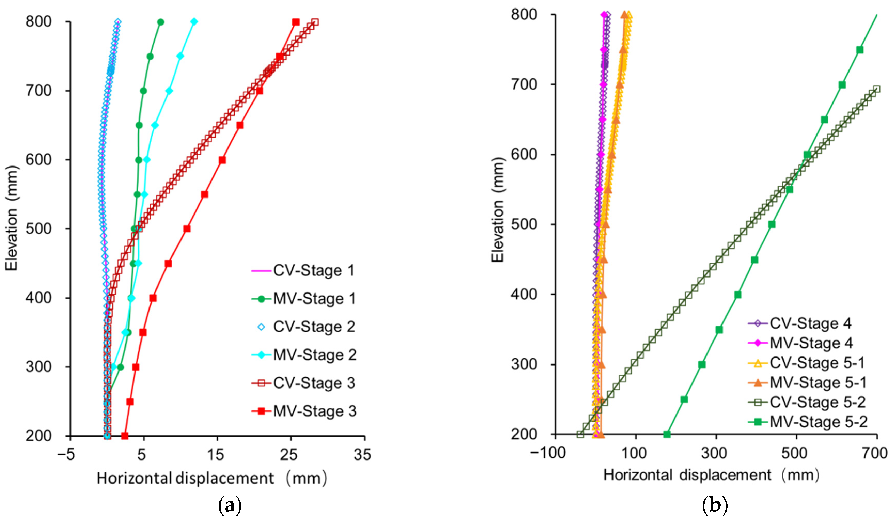
Figure 19 shows the calculated and measured horizontal displacement (HP) of the seaside pile in the five stages. In Stage 1, the dynamic wave pushed the top of the seaside pile landward, but the sand infill restricted the displacement and produced a slight seaward bulge, which was observed in both the calculated and measured HPs. The landside pile was pushed landward by the sand infill but restricted by the tie rods. Thus, there was also a slightly landward bulge in the landside pile (Figure 20). The difference in the HPs between Stages 1 and 2 was not very large due to the constraint of the sand infill. However, the HPs in both the seaside and landside piles largely increased in Stage 3 due to the taller breaking wave and erosions of the soil in the landside seabed and between the two piles. The largest calculated HPs were 28.2 mm in the seaside pile (vs. 25.7 mm in the measured HP) and 24.4 mm in the landside pile (vs. 16.6 mm in the measured HP).
In Stage 4, despite the higher water level of 73 cm, the HPs in both the seaside and landside piles did not change obviously due to the relatively small dynamic water wave. In Stage 5-1 with 8 cm high waves, the HPs of the seaside and landside piles increased to 82 mm (vs. 71.4 mm in the measured HP) and 78.1 mm (vs. 61.9 mm in the measured HP). In Stage 5-2, further soil erosion in the landside seabed greatly decreased the insertion depth of the landside pile, leading to failure of the DSSP cofferdam. The HPs of both the seaside and landside piles became very large, with 877 mm (vs. 694 mm in the measured HP) and 675 mm (vs. 464 mm in the measured HP), respectively.
4.3. The Stress of the Cofferdam
Figure 21 shows the calculated and measured stresses of the two piles in the five stages. In Stage 1, the stress curve of the seaside pile had an S-shape with the inflection point close to the seabed. The sand infill pushed the pile to bulge seaward above the seabed. In Stage 2, the larger wave action offset some deformation of the seaside pile and decreased the stress. The stresses of the landside pile in Stages 1 and 2 were small, which showed the relatively small static and dynamic water pressures that the seaside pile and sand infill underwent. In Stage 3, larger dynamic wave action and the soil erosion in the landside seabed deformed both piles in inverse S-shapes, which denoted good synergy between the two piles through the connections of the tie rods and the sand infill. In Stage 4, the stress in the seaside pile decreased under the smaller dynamic wave action because of the recovery of the elastic deformation under the larger dynamic wave in Stage 3. The stress on the landside did not change much. In Stage 5, the large dynamic wave pressure at a high water level pushed the DSSP to failure. The stresses in both piles became the largest.
Despite similar trends for the calculated and measured HPs and stresses, there were nonnegligible differences between them. The reason was that the soil in the seabed in the real tests underwent nonlinear plastic deformation during dynamic wave action, which was not simulated well by the finite element model with the ideal elastic–plastic constitutive of the Mohr–Coulomb model.
Both the tests and the numerical simulation showed that three external influence factors affected the HPs and stresses: static water pressure, dynamic wave impact, and soil erosion in the landside seabed. Static water pressure was the least significant factor, as the DSSP cofferdam as a whole had good stability and resistance to deformation. The dynamic wave impact, especially when the wave broke, had a larger influence on the DSSP, which forced the sheet pile to bend. However, the HPs and stresses on the two piles were still limited if no erosion occurred in the landside seabed or sand infill. Soil erosion led to the large HP and stresses and failure of the DSSP cofferdam. Therefore, reinforcement of the soil in the landside and sand infill to prevent erosion is of critical importance.
5. Discussion
5.1. Comparisons of the Dynamic Behavior of the Cofferdam with Difference Methods
Two methods are commonly applied for simulating dynamic wave action on structures: the quasi-static method (static method) and the pseudo-dynamic method (cyclic load method). The former treats the wave action as static load on the structure based on an empirical formula, and the latter treats the wave action as a regular periodical wave (e.g., cosine wave).
The pseudo-static method considers wave forces as static loads acting directly on structures, overlooking the dynamic variation characteristics of wave forces. Compared to dynamic analysis, the calculation process is simpler and more intuitive. The cyclic loading method simulates wave forces acting on structures in cycles according to the wave period, closely resembling the characteristics of actual wave actions. The dynamic time-history method, by inputting actual dynamic load time histories, analyzes the structure’s dynamic response, capable of simulating the structure’s nonlinear response under complex dynamic loads. The pseudo-static method simplifies dynamic problems into static issues, focusing mainly on the structure’s response under the most unfavorable conditions. The cyclic loading method introduces the periodicity of the load, closely approximating the real dynamic actions, but still operates under certain simplifying assumptions. The dynamic time-history method offers a comprehensive dynamic analysis, capable of detailed reflection on the structure’s time-varying behavior under dynamic actions.
Stage 3 was taken as an example to compare the two methods with the present method (PM). Figure 22 shows the inputs for the static method according to the Code of Hydrology for Harbour and Waterway [25] The input of the cyclic load method was set as a cosine wave on the basis of Figure 22.
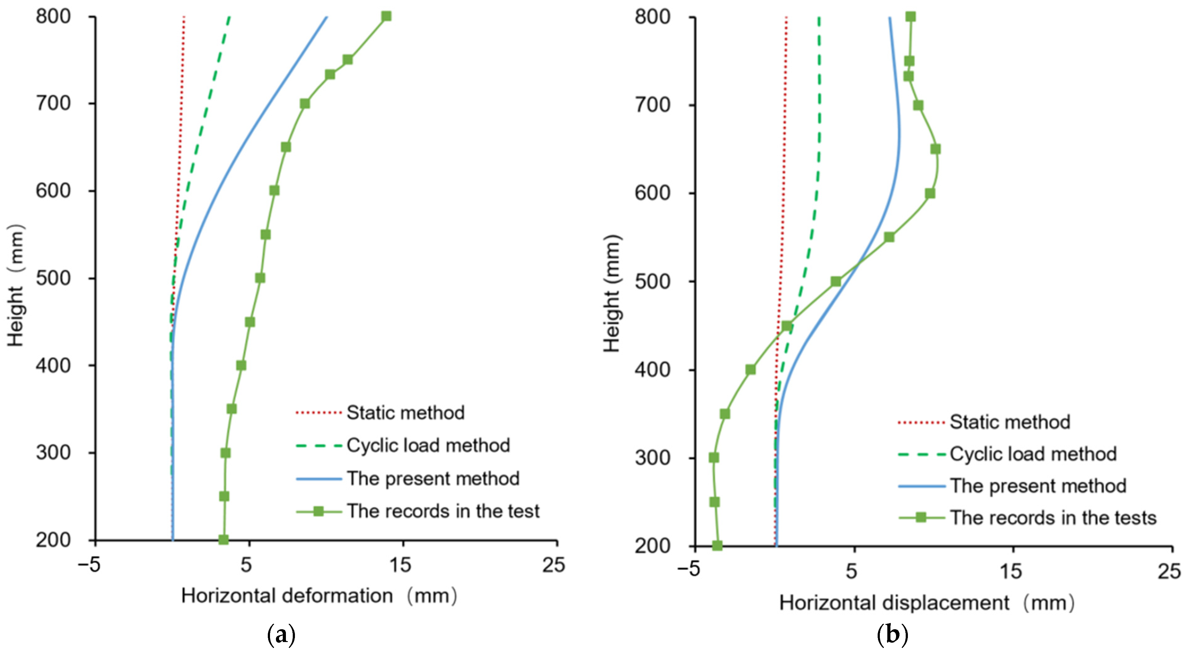
Figure 23 shows the calculated HP of the two steel sheet piles in Stage 3 before erosion in the landside seabed. The displacements with the static method were relatively small in both seaside and landside piles. The displacements with the cyclic load method were larger than those of the static method. The reason is that the dynamic load caused plastic deformation in the soils, which restricted the recovery of both piles. The HPs calculated via both the static method and cyclic load method were much smaller than the records in the test, as the large dynamic wave pressure caused by breaking waves was not properly simulated. In contrast, the HP calculated via the present method was much closer to the records because it considered the breaking waves. Despite this, there was still some difference between the calculated and measured HPs, especially in the foot of the piles. In the test, there was plastic deformation of 3–4 mm in both piles because of the tilt caused by the sand infill, which cannot be simulated by the finite element method with an ideal elastic–plastic constitutive equation.
5.2. Deformation of the DSSP Cofferdam in Tests and Simulation
Figure 24 shows the results of the simulation of the deformation of the DSSP cofferdam in the five stages as well as the corresponding snapshots in the tests. The soil erosion was modeled by removing the element meshes. Generally, the calculated results agreed well with the test values. It is found from the comparison analysis between numerical simulation and laboratory tests that the DSSP deformation dramatically increased when the landside soils were eroded by the leakage between the piles and glass wall and the overflow. The large wave (H = 8 cm) then pushed the cofferdam tilted with large displacement. The results emphasized the importance of sheet pile waterproofing, wave overflow prevention, and soil erosion on the landside as well as the top of the cofferdam.
5.3. Behavior of the DSSP Cofferdam with Reinforced Measures in Different Seabeds
In order to prevent the DSSP cofferdam from continuous failures of deformation–leakage–erosion–tilting, four reinforced measures were taken in sandy and clay interlay seabed foundations, as shown in Figure 25.
- (1)
- The seabeds close to both seaside and landside sheet piles were covered with geotextile bags filled with coarse sands to prevent soil erosion.
- (2)
- The height of the seaside sheet pile was increased 10 cm to reduce wave overflow.
- (3)
- The top of the cofferdam between the two piles was covered with clay packed with plastic bags to prevent soil erosion and water infiltration.
- (4)
- The junctions between the sheet piles and the glass walls were covered with clay for waterproofing.
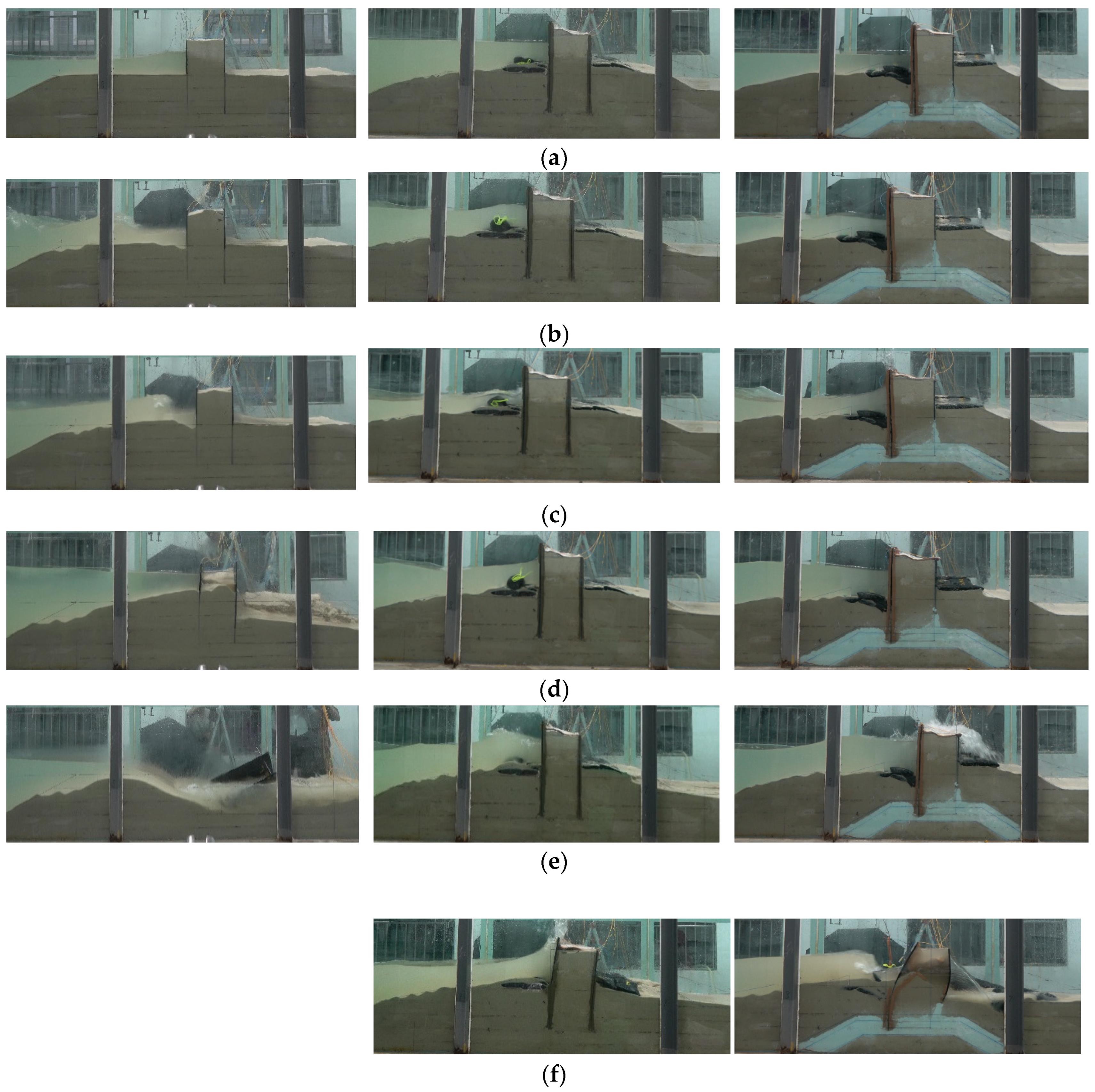
The effects of the reinforced measures were great as shown in the middle of Figure 26. The wave overflow was strongly mitigated by the higher landside steel pile. The leakage between the piles and the glass wall was very small because of the clay waterproofing. The upper part of the sands between two sheet piles remained dry. The soil erosions on the seabed of both seaside and landside were successfully controlled by the geotextile bag filled with coarse sands. Finally, the cofferdam did not fail at Stage 5 with water level of 73 cm and wave height of 8 cm. Moreover, the cofferdam successfully endured much larger waves with the height of 12 cm at Stage 6 as shown in the middle of Figure 26e, despite relatively large deformation.
When there is a clay interlayer seabed beneath the cofferdam and the pile end is inserted into a clay layer, the situation would be different, as shown in the right figures in Figure 26. The seaside pile sunk down into the soft clay layer, reducing the height of that pile. The textile bag close to the pile also sunk down. The cofferdam worked well when either the water level or the wave height was not very large. However, the wave overflow became very large when the water level and the wave height rose to 73 cm and 12 cm, respectively. The seabed soils as well as the textile bag were washed away. The landside pile tilted landward. With the constraint of the tie rods pulled by the seaside pile, the landside pile bent but stood up. Compared to Test 2 with a sandy seabed, the DSSP cofferdam in the clay interlayer seabed should have a higher wave wall due to large settlement cause by the soft clay.
5.4. Limitations
Although some results were obtained by experimental and numerical study on the stability of a DSSP cofferdam under wave surge action, there are still some limitations in the study.
- (1)
- The influence of wave period was not investigated in this study due to the workload. The wave height is varied from 4 cm to 12 cm, while the period is constant at 2 s. This is not an appropriate setting for natural waves. The effect of the wave period will be studied in the future work.
- (2)
- The effect of increased pressure due to wave breaking is pointed out in both laboratory tests and numerical simulation, but the characteristics of wave breaking are not quantitatively studied due to the complex mechanisms. Additionally, the importance of erosion in the failure process is mentioned, and the similarities of Shields number and shear velocity were not examined, especially the dynamic erosion due to wave action.
- (3)
- The numerical analysis method used in this study is not truly a coupled method of CFD and FEM, and the mesh for erosion was removed manually. In addition, since the topographic change is expected to be affected by the reduction of soil strength due to liquefaction, the dynamic behavior of the pile model also needs to be discussed in the future.
6. Conclusions
In this study, the dynamic behavior of a DSSP cofferdam under wave action was studied through a large-scale flume test and a numerical simulation that combined CFD and FEM. The effect of the reinforced measures was investigated in both sandy and clay seabed. The following conclusions were drawn:
- (1)
- The waves caused erosion and deposition in the seaside seabed, forming a slope inclined in the seaward direction. The angle of the slope increased with the wave height, decreasing the water depth close to the seaside pile. The tall waves and shallow water depth made the waves break, significantly increasing the dynamic wave pressure toward the seaside pile and the overflow volume.
- (2)
- The static water pressure caused the stress of the seaside pile to increase in the middle part. Small waves increased the stress in the bottom part of the seaside pile and continuous unrecoverable plastic deformation in the seabed soils. The breaking waves dramatically increased the stress and displacement of the seaside pile due to the large dynamic pressure. The erosion of the landside seabed made the stress and deformation of the landside pile the largest. The stresses on the tie rods depended on the relative displacement of the two piles, which showed that the effect of the tie rods maintained the DSSP cofferdam as a whole structure.
- (3)
- Despite the waterproof DSSP, the seepage from the high water head made the landside slope slide. The dynamic wave pressure accelerated the seepage and caused excess pore water pressure. The higher the wave was, the larger the excess pore water pressure. The overlap of the traveling and the reflected waves increased the excess pore water pressure in the area close to the seaside pile due to the taller overlapped wave and higher wave frequency.
- (4)
- The DSSP cofferdam failed under the combined action of the dynamic wave pressure and the erosion of the landside seabed and sand infill between the two piles. The dynamic wave pressure caused large deformation of the piles, leading to leakage between the glass wall and the piles. The leakage and overflow of the breaking waves resulted in significant erosion of the landside seabed and the sand infill, greatly weakening the support of the seabed. The dynamic wave pressure then pushed the DSSP cofferdam to failure.
- (5)
- The results of the simulation with the combined methods of CFD and FEM had trends that were similar to those of the measurement results in the tests. Compared to the quasi-static method and pseudo-dynamic method, the results of the simulation via the present method were much closer to the experimental measurements because the simulation included the dynamic wave pressure increase caused by breaking waves.
- (6)
- According to the deformation–leakage–erosion–tilting continuous failure mechanisms of the DSSP cofferdam, four reinforced measures were taken to reduce the wave overflow, leakage, and soil erosion. The reinforced DSSP cofferdam not only endured the maximal wave load in the tests but also stayed stable in even larger wave load. Meanwhile, the DSSP cofferdam in a clay interlayer seabed should have a higher wave wall due to large settlement caused by the soft clay.
Author Contributions
Y.Z.: Conceptualization, writing—original draft, calculation, and analysis; J.B.: Review and editing, methodology, and resources; H.X.: Review and editing, methodology, and resources; M.P.: Conceptualization, supervision, methodology, funding acquisition, and reviewing; Y.H.: Conceptualization, methodology, review and editing, and resources; K.W.: Writing—review and editing and resources; X.P.: Review and editing. All authors have read and agreed to the published version of the manuscript.
Funding
The research reported in this paper was substantially sponsored by the Program of Shanghai Academic/Technology Research Leader (23XD1434800), the National Natural Science Foundation of China (Nos. 42207238, 42177137, 42071010, 42061160480), the Program of Shanghai Science and Technology Commission (21DZ2207200), and the Shanghai Natural Science Foundation (20ZR1461300).
Data Availability Statement
Data are contained within the article.
Conflicts of Interest
Authors Yan Zhu, Jingchao Bi, Kaifang Wang, and Xinyu Pan were employed by China Shipbuilding NDRI Engineering Co., Ltd. The remaining authors declare that the research was conducted in the absence of any commercial or financial relationships that could be construed as a potential conflict of interest.
References
- Gönnert, G.; Gerkensmeier, B. A multi-method approach to develop extreme storm surge events to strengthen the resilience of highly vulnerable coastal areas. Coast. Eng. J. 2015, 57, 1540002. [Google Scholar] [CrossRef]
- Wahl, T.C.; Mudersbach, J. Statistical assessment of storm surge scenarios within integrated risk analyses. Coast. Eng. J. 2015, 57, 1540003. [Google Scholar] [CrossRef]
- Streicher, M.; Kortenhaus, A.; Marinov, K.; Hirt, M.; Hughes, S.; Hofland, B.; Schüttrumpf, H. Classification of bore patterns induced by storm waves overtopping a dike crest and their impact types on dike mounted vertical walls—A large-scale model study. Coast. Eng. J. 2019, 61, 321–339. [Google Scholar] [CrossRef]
- Toyoda, M.; Fukui, N.; Miyashita, T.; Shimura, T.; Mori, N. Uncertainty of storm surge forecast using integrated atmospheric and storm surge model: A case study on Typhoon Haishen 2020. Coast. Eng. J. 2022, 64, 135–150. [Google Scholar] [CrossRef]
- Gui, M.W.; Han, K.K. An investigation on a failed double-wall cofferdam during construction. Eng. Fail. Anal. 2009, 16, 421–432. [Google Scholar] [CrossRef]
- Furuichi, H.; Hara, T.; Tani, M.; Nishi, T.; Otsushi, K.; Toda, K. Study on reinforcement method of dykes by steel sheet-pile against earthquake and tsunami disasters. Soil Eng. J. 2015, 10, 583–594. (In Japanese) [Google Scholar]
- Cheng, X.S.; Zheng, G.; Diao, Y.; Huang, T.M.; Deng, C.H.; Lei, Y.W.; Zhou, H.Z. Study of the progressive collapse mechanism of excavations retained by cantilever contiguous piles. Eng. Fail. Anal. 2017, 71, 72–89. [Google Scholar] [CrossRef]
- Wang, K.Z.; Gao, Y.H.; Jin, Z.H.; Zhou, X.; Chen, L.H.; Zhang, C. Research on stability of steep bank slope and reserved thin-walled rock cofferdam during excavation of intake foundation pit. Eng. Fail. Anal. 2022, 141, 106659. [Google Scholar] [CrossRef]
- Yi, F.; Su, J.; Zheng, G.; Cheng, X.S.; Zhang, J.T.; Lei, Y.W. Overturning progressive collapse mechanism and control methods of excavations retained by cantilever piles. Eng. Fail. Anal. 2022, 140, 106591. [Google Scholar] [CrossRef]
- Kimura, M.; Inazumi, S.; Too, J.K.A.; Isobe, K.; Mitsuda, Y.; Nishiyama, Y. Development and application of H-joint steel pipe sheet piles in construction of foundations for structures. Soils Found. 2007, 47, 237–251. [Google Scholar] [CrossRef]
- Mawer, R.W.; Byfield, M.P. Reduced modulus action in U-section steel sheet pile retaining walls. J. Geotech. Geoenviron. Eng. 2010, 136, 439–444. [Google Scholar] [CrossRef]
- Inazumi, S.; Kimura, M.; Kakuda, T.; Kobayashi, M. Water cut-off performance of H-jointed steel pipe sheet piles with HH joints attaching water-swelling materials. Soils Found. 2011, 51, 1019–1035. [Google Scholar] [CrossRef]
- Wang, J.F.; Xiang, H.W.; Yan, J.G. Numerical simulation of steel sheet pile support structures in foundation pit excavation. International Journal of Geomechanics. Int. J. Geomech. 2019, 19, 05019002. [Google Scholar] [CrossRef]
- Osthoff, D.; Grabe, J. Deformational behaviour of steel sheet piles during jacking. Comput. Geotech. 2018, 101, 1–10. [Google Scholar] [CrossRef]
- Kang; Zhu, B.; Lin, P.; Ju, J.; Zhang, J.; Zhang, D. Experimental and numerical study of wave-current interactions with a dumbbell-shaped bridge cofferdam. Ocean Eng. 2020, 210, 107433. [Google Scholar] [CrossRef]
- Ohori, K.; Takahashi, K.; Kawai, Y.; Shiota, K. Static analysis model for double sheet-pile wall structures. J. Geotech. Eng. ASCE 1988, 114, 810–825. [Google Scholar] [CrossRef]
- Khan, M.R.A.; Takemura, J.; Kusakabe, O. Centrifuge model tests on behavior of double sheet pile wall cofferdam on clay. Int. J. Phys. Model. Geotech. Model. Geotech. 2006, 6, 1–23. [Google Scholar] [CrossRef]
- Hou, Y.M.; Wang, J.H.; Gu, Q.Y. Deformation performance of double steel sheet piles cofferdam. J. Shanghai Jiaotong Univ. 2009, 43, 1577–1580. [Google Scholar]
- Mitobe, Y.; Adityawan, M.B.; Roh, M.; Tanaka, H.; Otsushi, K.; Kurosawa, T. Experimental study on embankment reinforcement by steel sheet pile structure against tsunami overflow. Coast. Eng. J. 2016, 58, 1640018-1–1640018-18. [Google Scholar] [CrossRef]
- Zhu, Y.; Gu, Q.Y.; Jiang, J.; Peng, M. Reliability analysis for overall stability of large-span double-row steel sheet-piled dock cofferdam based on Bayesian method. Rock Soil Mech. 2016, 37, 609–615. (In Chinese) [Google Scholar]
- Fujiwara, K.; Taenaka, S.; Otsushi, K.; Yashima, A.; Sawada, K.; Ogawa, T.; Takeda, K. Study on levee reinforcement using double sheet-piles with partition walls. Jpn. Geotech. Soc. Spec. Publ. 2017, 5, 11–15. [Google Scholar]
- Xue, R.Z.; Bie, S.A.; Guo, L.L.; Zhang, P.L. Stability analysis for cofferdams of pile wall frame structures. KSCE J. Civ. Eng. 2019, 23, 4010–4021. [Google Scholar] [CrossRef]
- Peng, M.; Li, Z.; Zhu, Y.; Zhang, J.L. Stability analysis of double-row steel sheet pile cofferdam with sandy and cohesive foundation under surge wave action. Geo-Risk 2023 Dev. Reliab. Risk Resil. 2023, 346, 195–203. [Google Scholar]
- Boltzmann, L. Weitere studien über das wärmegleichgewicht unter gasmolekülen. In Kinetische Theorie II; Springer: Berlin/Heidelberg, Germany, 1970. [Google Scholar]
- JTS 145-2015; Code of Hydrology for Harbour and Waterway. Ministry of Transport of the People’s Republic of China: Beijing, China, 2022.
Figure 1.
Test setup: (a) the test flume; (b) wave-generating machine; (c) wave-generating board; (d) control computer and data collection system.
Figure 1.
Test setup: (a) the test flume; (b) wave-generating machine; (c) wave-generating board; (d) control computer and data collection system.

Figure 2.
The cross-section of the cofferdam at the Changxing dock.

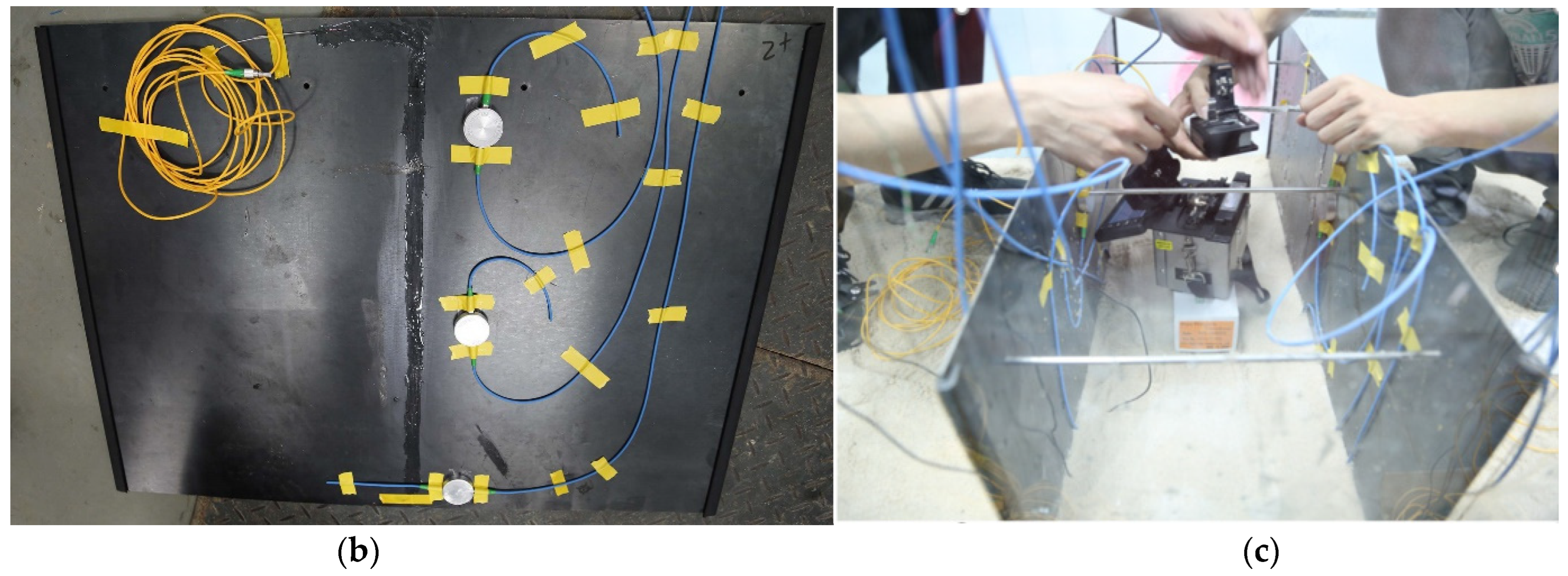
Figure 3.
The model cofferdam with double-wall steel sheet piles: (a) the cofferdam model; (b) the steel sheet pile with monitoring sensors; (c) two steel sheet piles connected with four tie rods.
Figure 3.
The model cofferdam with double-wall steel sheet piles: (a) the cofferdam model; (b) the steel sheet pile with monitoring sensors; (c) two steel sheet piles connected with four tie rods.


Figure 4.
Experimental setup and measurement system layout: (a) full side view; (b) side view; (c) top view.
Figure 4.
Experimental setup and measurement system layout: (a) full side view; (b) side view; (c) top view.

Figure 5.
Wave production process in the model test.

Figure 6.
Snapshot of the pre-wave stage: (a) at 11′06″; (b) at 29′04″; (c) at 43′33″. Note: the left photos show the side view, and the right photos show the seaward view from the landside.
Figure 6.
Snapshot of the pre-wave stage: (a) at 11′06″; (b) at 29′04″; (c) at 43′33″. Note: the left photos show the side view, and the right photos show the seaward view from the landside.

Figure 7.
Stresses of the steel sheet piles and the tie rods based on results from fiber optic sensors and pore water pressure: (a) offshore side pile, (b) landside pile, (c) tie rod, (d) the pore water pressure (the positions of the monitor points are shown as OP, LP, PR, and P in Figure 4). Note: Point 0 was the moment of starting to add water at 0 s; Point A was the moment when the water level reached 50 cm (the top of the seabed) at 10 min; Point B was the moment when the wave (wave height = 4 cm) was generated at 47 min (water level = 65 cm); Point C was the moment when the wave (wave height = 8 cm) was generated at 63 min (water level = 65 cm); Point D was the moment when the wave started to break at 69 min; Point E was the moment when the wave (wave height = 12 cm) was generated at 77 min (water level = 65 cm); Point F was the moment when the 12 cm high wave ended at 85 min; Point G was the moment when the wave (wave height = 4 cm) was generated at 100 min (water level = 73 cm); Point H was the moment when the wave (wave height = 8 cm) was generated at 115 min (water level = 73 cm).


Figure 8.
Snapshot of Stage 1 with water depth of 65 cm and wave height of 4 cm: (a) at 47′16″; (b) at 55′20″; (c) at 61′45″. Note: the left photos show the top view, the middle photos show the side view, and the right photos show the seaward view from landside.
Figure 8.
Snapshot of Stage 1 with water depth of 65 cm and wave height of 4 cm: (a) at 47′16″; (b) at 55′20″; (c) at 61′45″. Note: the left photos show the top view, the middle photos show the side view, and the right photos show the seaward view from landside.

Figure 9.
Snapshot of Stage 2 with water depth of 65 cm and wave height of 8 cm: (a) at 64′36″; (b) at 68′25″; (c) at 73′08″. Note: the left photos show the top view, the middle photos show the side view, and the right photos show the seaward view from the landside.
Figure 9.
Snapshot of Stage 2 with water depth of 65 cm and wave height of 8 cm: (a) at 64′36″; (b) at 68′25″; (c) at 73′08″. Note: the left photos show the top view, the middle photos show the side view, and the right photos show the seaward view from the landside.

Figure 10.
Snapshot of Stage 3 with water depth of 65 cm and wave height of 12 cm: (a) at 77′58″; (b) 81′51″; (c) 84′54″. Note: the left photos denote the top view, the middle photos show the side view, and the right photos show the seaward view from the landside.
Figure 10.
Snapshot of Stage 3 with water depth of 65 cm and wave height of 12 cm: (a) at 77′58″; (b) 81′51″; (c) 84′54″. Note: the left photos denote the top view, the middle photos show the side view, and the right photos show the seaward view from the landside.

Figure 11.
Snapshot of Stage 4 with water depth of 73 cm and wave height of 4 cm: (a) at 100′44″; (b) at 106′20″; (c) at 112′37″. Note: the left photos show the top view, the middle photos show the side view, and the right photos show the seaward view from the landside.
Figure 11.
Snapshot of Stage 4 with water depth of 73 cm and wave height of 4 cm: (a) at 100′44″; (b) at 106′20″; (c) at 112′37″. Note: the left photos show the top view, the middle photos show the side view, and the right photos show the seaward view from the landside.


Figure 12.
Snapshot of Stage 5 with water depth of 73 cm and wave height of 8 cm: (a) at 115′03″; (b) at 115′58″; (c) at 116′54″; (d) at 117′05″. Note: the left photos show the top view, the middle photos show the side view, and the right photos show the seaward view from the landside.
Figure 12.
Snapshot of Stage 5 with water depth of 73 cm and wave height of 8 cm: (a) at 115′03″; (b) at 115′58″; (c) at 116′54″; (d) at 117′05″. Note: the left photos show the top view, the middle photos show the side view, and the right photos show the seaward view from the landside.

Figure 13.
The failure process of the DSSP cofferdam in Stage 5. Note: the black lines are the steel sheet piles and tie rod, and the dotted lines are the soil envelope of the seabed and the sand infill before wave generation.
Figure 13.
The failure process of the DSSP cofferdam in Stage 5. Note: the black lines are the steel sheet piles and tie rod, and the dotted lines are the soil envelope of the seabed and the sand infill before wave generation.

Figure 14.
Force analysis of the DSSP cofferdam under wave action: (a) force components; (b) simulation.
Figure 14.
Force analysis of the DSSP cofferdam under wave action: (a) force components; (b) simulation.

Figure 15.
The wave conditions of the five stages in the Kolmar diagram.

Figure 16.
Numerical model of the cofferdam flume tests under wave action. Note: the seaside pile was separated into six segments of 5 cm each, and the dynamic wave pressure was added to each segment.
Figure 16.
Numerical model of the cofferdam flume tests under wave action. Note: the seaside pile was separated into six segments of 5 cm each, and the dynamic wave pressure was added to each segment.

Figure 17.
Snapshot of the velocity distribution of the wave in Stage 3 with water depth of 65 cm and wave height of 12 cm: (a) with a trough on the seaside pile; (b) with crest on the seaside pile.
Figure 17.
Snapshot of the velocity distribution of the wave in Stage 3 with water depth of 65 cm and wave height of 12 cm: (a) with a trough on the seaside pile; (b) with crest on the seaside pile.

Figure 18.
Part of the time records of the wave force in the five stages.

Figure 19.
The horizontal displacement of the seaside pile: (a) with water depth of 65 cm, (b) with water depth of 73 cm. Note: CV = calculated value, MV = measured value. Stage 5 was divided into two sub-stages by considering the soil erosion: Stage 5-1 (with erosion depth of 4 cm) and Stage 5-2 (with erosion depth of 8 cm), as shown in Figure 18.

Figure 20.
The horizontal displacement of the landside pile: (a) with water depth of 65 cm, (b) with water depth of 73 cm. Note: CV = calculated value, MV = measured value.
Figure 20.
The horizontal displacement of the landside pile: (a) with water depth of 65 cm, (b) with water depth of 73 cm. Note: CV = calculated value, MV = measured value.

Figure 21.
The measured and calculated stresses at the end of the five stages: (a) seaside pile, (b) landside pile. Note: CS = calculated stress, MS = measured stress.
Figure 21.
The measured and calculated stresses at the end of the five stages: (a) seaside pile, (b) landside pile. Note: CS = calculated stress, MS = measured stress.

Figure 22.
The input of the static method. Note: the input of the cyclic load method was set as a cosine wave on the basis of this figure.
Figure 22.
The input of the static method. Note: the input of the cyclic load method was set as a cosine wave on the basis of this figure.

Figure 23.
Horizontal deformation of the steel sheet piles in Stage 3 before erosion in the landside seabed: (a) the seaside pile; (b) the landside pile.
Figure 23.
Horizontal deformation of the steel sheet piles in Stage 3 before erosion in the landside seabed: (a) the seaside pile; (b) the landside pile.

Figure 24.
The deformation of the DSSP cofferdam and the seabed during the failure process: (a) at the end of Stage 1; (b) at the end of Stage 2; (c) at the end of Stage 3; (d) at the end of Stage 4; (e) failure at Stage 5. Note, the figures are the snapshots of the model tests, the blue line represents the deformed double row steel sheet piles, and the black line is the rigid tie rod in the simulation results for comparison.

Figure 25.
Layout of the DSSP cofferdam with reinforced measures in different seabeds: (a) with sandy seabed foundation; (b) with clay interlayer seabed foundation.
Figure 25.
Layout of the DSSP cofferdam with reinforced measures in different seabeds: (a) with sandy seabed foundation; (b) with clay interlayer seabed foundation.

Figure 26.
Snapshots of the DSSP cofferdams with reinforced measurement in different seabeds: (a) Stage 0; (b) at end of Stage 1 (D = 65 cm, H = 4 cm); (c) at end of Stage 2 (D = 65 cm, H = 8 cm); (d) at end of Stage 4 (D = 73 cm, H = 4 cm); (e) at end of Stage 5 (D = 73 cm, H = 8 cm); (f) at end of Stage 6 (D = 73 cm, H = 12 cm). Note: the figures on the left denote the test in sandy seabed without reinforced measures (Test 1); the figures in the middle denote the test in sandy seabed with reinforced measures (Test 2); and the figures on the right denote the test in clay interlayer seabed with reinforced measures (Test 3). The cofferdam in Test 1 failed at Stage 5 so there was no snapshot at Stage 6.


Table 1.
Properties of quartz sands in the seabed and between the piles.
| Description | Value |
|---|---|
| Sand (%) | 100 |
| Specific gravity | 2.4 |
| Maximum dry density (kg/m3) | 1444 |
| Minimum dry density (kg/m3) | 1240 |
| Average dry density (kg/m3) | 1403 |
| Soil friction angle at average density | 30.5° |
Table 2.
Hydraulic parameters in the 5 test stages.
| Stage | Water Depth, D (cm) | Wave Height, H (cm) | Period, T (s) | Wave Length, L (cm) |
|---|---|---|---|---|
| 1 | 65 | 4 | 2 | 450 |
| 2 | 65 | 8 | 2 | 450 |
| 3 | 65 | 12 | 2 | 450 |
| 4 | 73 | 4 | 2 | 470 |
| 5 | 73 | 8 | 2 | 470 |
Table 3.
The wave surface functions and velocity potential functions in the five tests.
| Test No. | Function Type | Function of the Wave |
|---|---|---|
| 1 | WSF | |
| VPF | ||
| 2 | WSF | |
| VPF | ||
| 3 | WSF | |
| VPF | ||
| 4 | WSF | |
| VPF | ||
| 5 | WSF | |
| VPF |
Note: WSF = wave surface function; VPF = velocity potential function.
Table 4.
Numerical simulation parameters for the fill material.
| Test Condition | Relative Compactness of Backfill Sand (Dr) | Cofferdam Width S (cm) | Tie Rod Height (cm) | γ (kN/m3) | Eref (MPa) | ν | C (kPa) | Φ (°) |
|---|---|---|---|---|---|---|---|---|
| Standard condition | 0.80 | 20.00 | 4.00 | 16.00 | 25.00 | 0.30 | 2.50 | 30.10 |
Table 5.
Parameters related to the model steel sheet piles.
| Material | Material Type | EA (1 × 10⁶ kN/m) | EI (kN·m2/m) | Thickness d (mm) | Unit Weight w (kN·m/m) |
|---|---|---|---|---|---|
| Steel plates | Linear elasticity | 1.14 | 2.38 | 5.00 | 78.00 |
Table 6.
Parameters related to the model tie rods.
| Material | Material Type | EA (1 × 10² kN) | Interval L (cm) |
|---|---|---|---|
| Galvanized iron wire | Linear elasticity | 3.00 | 8.00 |
Disclaimer/Publisher’s Note: The statements, opinions and data contained in all publications are solely those of the individual author(s) and contributor(s) and not of MDPI and/or the editor(s). MDPI and/or the editor(s) disclaim responsibility for any injury to people or property resulting from any ideas, methods, instructions or products referred to in the content. |
© 2024 by the authors. Licensee MDPI, Basel, Switzerland. This article is an open access article distributed under the terms and conditions of the Creative Commons Attribution (CC BY) license (https://creativecommons.org/licenses/by/4.0/).
Share and Cite
MDPI and ACS Style
Zhu, Y.; Bi, J.; Xing, H.; Peng, M.; Huang, Y.; Wang, K.; Pan, X. Stability Analysis of Cofferdam with Double-Wall Steel Sheet Piles under Wave Action from Storm Surges. Water 2024, 16, 1181. https://doi.org/10.3390/w16081181
AMA Style
Zhu Y, Bi J, Xing H, Peng M, Huang Y, Wang K, Pan X. Stability Analysis of Cofferdam with Double-Wall Steel Sheet Piles under Wave Action from Storm Surges. Water. 2024; 16(8):1181. https://doi.org/10.3390/w16081181
Chicago/Turabian StyleZhu, Yan, Jingchao Bi, Haofeng Xing, Ming Peng, Yu Huang, Kaifang Wang, and Xinyu Pan. 2024. "Stability Analysis of Cofferdam with Double-Wall Steel Sheet Piles under Wave Action from Storm Surges" Water 16, no. 8: 1181. https://doi.org/10.3390/w16081181
Note that from the first issue of 2016, this journal uses article numbers instead of page numbers. See further details here.