Research on the Prediction of Infiltration Depth of Xiashu Loess Slopes Based on Particle Swarm Optimized Back Propagation (PSO-BP) Neural Network

Abstract

The Xiashu loess exhibits expansion when in contact with water and contraction when water is lost, making it highly susceptible to the influence of rainfall. Therefore, it is essential to investigate the infiltration behavior of rainwater in Xiashu loess slopes under various conditions. The depth of infiltration in slopes directly affects the depth of landslide failure and serves as an important indicator for studying slope infiltration characteristics; only a handful of academics have delved into its study. This article is based on on-site rainfall experiments on Xiashu loess slopes, using three main factors, rainfall intensity, rainfall duration, and slope angle, as discrimination indicators for the infiltration depth of Xiashu loess slopes. The particle swarm optimization algorithm is employed to optimize the BP neural network and establish a PSO-BP neural network prediction model. The experimental data are accurately predicted and compared with the multivariate nonlinear regression model and traditional BP neural network models. The results demonstrate that the PSO-BP neural network model exhibits a better fit and higher prediction accuracy than the other two models. This model provides a novel approach for rapidly determining the infiltration depth of Xiashu loess slopes under different rainfall conditions. The results of this study lay the foundation for the prediction of the landslide damage depth and infiltration of Xiashu loess slopes.

1. Introduction

Studies indicate that since the 21st century, landslides have emerged as a major geological challenge for China [1]. Rainwater infiltration leads to erosion of the slope’s surface and the softening of its internal rock and soil, diminishing its stability and triggering landslides, with the Xiashu loess landslide being a common example. The Xiashu loess is mainly distributed in the area of Nanjing and Zhenjiang, Jiangsu Province [2], which poses a great threat to the safety issues of people’s lives and properties in the region. The Xiashu loess has characteristics such as swelling when encountering water and shrinking when losing water [3], which is significantly affected by rainfall and is prone to landslides in the rainy season. Therefore, it is crucial to study the infiltration characteristics of the Xiashu loess slopes under rainfall conditions.

Lately, an increasing number of academics have delved into the issues associated with the Xiashu loess. Hu et al. [4,5] studied the failure modes of the Xiashu loess under different moisture contents through experiments and investigated the infiltration pattern and damage mechanism of Xiashu loess slopes under different rainfall conditions; Liu et al. [6] researched the changes in mechanical properties of the Xiashu loess after undergoing different wet and dry cycles through unsaturated direct shear tests; Chen et al. [7] revealed the seismic response mechanism of Xiashu loess slopes through large-scale shaking table tests on the Xiashu loess; Sun et al. [8] experimentally analyzed a large number of Xiashu loess samples and found that the slope stability of the Xiashu loess is mainly affected by the soil water content. It can be seen that research on landslides in the Xiashu loess has focused on analyzing the causes of landslides as well as on early warning, and less research has been conducted on the depth of infiltration of Xiashu loess slopes under rainfall conditions.

For other soil slopes, some scholars have explored the infiltration depth of slopes under different rainfall conditions through simulated rainfall experiments [9,10] but have not conducted predictive research. At present, in the prediction of slopes, most scholars focus on the prediction of slope deformation and stability [11,12,13,14,15], and there are few studies on the prediction of landslide damage depth [16]. Landslide damage depth is affected by a variety of factors [17], its uncertainty is higher, and it is more difficult to predict directly. Some scholars believe that shallow landslides parallel to the surface of soil slopes often occur (failure at wet fronts) [18,19]; thus, the range of landslide damage depths can be indirectly determined from rainfall infiltration depths and the prediction of slope infiltration depths is better implementable.

Various methods are employed for prediction, including support vector machine, neural networks, extreme learning machine, multiple regression, etc. Each method has its own set of advantages and disadvantages, and they have collectively yielded improved prediction results [20,21,22,23]. The above method can realize the rapid estimation of landslide characteristics by building a prediction model, which is different from the traditional numerical simulation analysis method because of its high efficiency and excellent prediction accuracy [24]. Among these, neural networks are utilized to establish relationships between variables by simulating biological neural networks. They possess a strong capability to accommodate nonlinearity and exhibit autonomous learning, making them widely employed in slope prediction research. However, it also has limitations, such as the issue of too rapid a convergence and the susceptibility to becoming trapped in local minima [25]. In order to make up for the deficiencies in neural networks, many scholars have used different algorithms to optimize neural networks, and these algorithms include the Genetic Algorithm [26,27], Bird Swarm Algorithm [28], particle swarm algorithm [29,30,31], Sparrow Algorithm, etc., which are all able to overcome the limitations of local optimums and assign optimized weights and thresholds to the neural network to improve the prediction accuracy of the neural network. In this paper, based on the experimental situation, we consider optimizing the BP neural network with the particle swarm algorithm (PSO) to make up for the shortcomings of the neural network, so that the optimized neural network has a better prediction effect [32,33]. This study forecasts the infiltration depth of Xiashu loess slopes using a BP neural network enhanced by the particle swarm algorithm (PSO), aiming to clarify the relationship between rainfall duration, rainfall intensity, slope angle, and the depth of slope infiltration. Concurrently, a comparison is made between the PSO-BP neural network model, the multivariate nonlinear regression prediction model, and the unoptimized BP neural network to evaluate the pros and cons of these models and to formulate the prediction model effectively. A rapid method for determining the infiltration depth of Xiashu loess slopes is proposed to provide the basis for the subsequent prediction of landslide damage depth and infiltration studies of Xiashu loess slopes.

2. Methodology

2.1. Principles of Multivariate Nonlinear Regression Model

Regression analysis is a quantitative depiction of uncertain relationships between things that exist in the objective world with the help of mathematical models. In the analysis of a nonlinear link between a dependent variable Y and one or several independent variables (X₁~X_n), employing a nonlinear regression model is feasible, along with the use of statistical analysis techniques and functions for the analytical interpretation and formal depiction of the relationship. The multiple regression equation allows the relationship between input and output values to be established in order to quickly and efficiently estimate the output values from the input values. Based on the output values, this information is useful for risk assessment. In nonlinear regression models, least-squares stands as the predominant technique for estimating parameters, and the models developed through this approach are considered a posteriori models in the realm of statistical mathematical modeling. This technique is applicable for forecasting the depth of rainfall infiltration on slopes, employing a linear function to mimic a nonlinear function, and repeating this method to achieve the best parameter solution.

Presently, two primary varieties of nonlinear mathematical models exist, linking several independent variables with a single dependent variable. In Type I nonlinear mathematical models, the initial step is to examine the functional link between an independent variable and its dependent counterpart independently, followed by overlaying this connection between the dependent and independent variables. Should the overlaid functional link fail to meet specific criteria, it becomes essential to delve deeper into the interplay among the independent variables. Nonlinear mathematical models of Type I are straightforward, highly suitable, and broadly applicable. In contrast, Type II nonlinear mathematical models have been less applied by scholars due to their excessive complexity. Thus, the considered nonlinear mathematical models are currently dominated by Type I. The mathematical expression for the nonlinear mathematical model of Type I is given in the following equation:

$$y=k_0+{\sum }_{i=1}^n{k}_i{f}_i\left(x_i\right)+{\sum }_{i=1}^n{k}_j{x}_i{x}_j,$$

(1)

where $y$ is the dependent variable; $k_i$ is the regression coefficient; $x_i$ and x_j are independent variables, i = 0,⋯, n; j = 0,⋯, n; and $f_i\left(x_i\right)$ is the functional relationship between a particular independent variable and the dependent variable.

2.2. Principles of BP Neural Network

Developed in the 1980s, BP neural networks have found extensive application among researchers in control, optimization, and nonlinear prediction, owing to their straightforward design and user-friendliness. Neural networks reflect the structure and function of the human brain’s nerves, abstracting the properties of the real brain and simplifying it into an information processing system. Typically, a BP neural network is composed of three distinct layers: input, hidden, and output layers. The learning principle is as follows: During forward propagation, a set of weights and thresholds is randomly generated. This set of randomly generated numbers, along with the excitation function, jointly act on the input parameters. The input parameters are passed from the input layer to the output layer through the implicit layer. The output value is compared to the expected value. If the error between the two exceeds the accepted range, the error is back-propagated from the output layer. The initial randomly generated weights and thresholds are then adjusted and corrected to continue the learning process through continuous iterative learning. This process continues until the final output value and the expected value have an error within an acceptable range. At this point, the training ends. Research has demonstrated that a tri-layered BP neural network meets the criteria for general function mapping, and various multivariate functions can be estimated with any desired precision using a limited set of hidden-layer BP neural networks. The structure of the BP neural network is shown in Figure 1.

2.3. Particle Swarm Optimization

Eberhart and Kennedy jointly introduced the particle swarm optimization (PSO) algorithm in 1995, drawing inspiration from the collective food-seeking patterns of animal birds. This algorithm mimics bird foraging for group iteration and seeks the most suitable area within the particle group to identify the optimal particles for the desired solution space. Each particle in the algorithm represents a solution. The initial state of all particles in the population is continuously iterated. At each iteration, the particles update themselves to keep track of the optimal value, in order to find the optimal solution.

The particle swarm algorithm begins by initializing a group of random particles. Assuming there are m particles in the swarm, each particle has an n-dimensional vector that represents a solution in the n-dimensional optimization space. X_j represents the positional vector for particle j, and V_j denotes the velocity vector for particle j.

$$X_j=X_{j1},X_{j2},\cdots X_{jn},$$

(2)

$$V_j=V_{j1},V_{j2},\cdots V_{jn},$$

(3)

In the iterative phase, vectors representing particle positions are integrated into the fitness function E_k to obtain their fitness values. The optimal fitness values of the particles are compared to search for the particle swarm’s successive single best position P_j and global best position G_j.

$$P_j=P_{j1},P_{j2},\cdots ,P_{jn},$$

(4)

$$G_j=G_{j1},G_{j2},\cdots ,G_{jn},$$

(5)

The individual optimal solution achieved by each particle during the search process is represented by P_j, while the global optimal solution achieved by the particles during the search process, the optimal solution of the particle swarm algorithm, is represented by G_j. The particle swarm algorithm updates and optimizes based on four values: X_j, V_j, P_j, and G_j. These values are used to determine the position and velocity vectors after each iteration, with the algorithm’s evolution equation being

$$V_j\left(k+1\right)=w\cdot V_j\left(k\right)+c_1\cdot r_1\cdot \left[P_j\left(k\right)-X_j\left(k\right)\right]+c_2\cdot r_2\cdot \left[G_j\left(k\right){-X}_j\left(k\right)\right],$$

(6)

$$X_j(k+1)=X_j\left(k\right)+V_j(k+1),$$

(7)

where $w$ is the inertia weight; $c_1$ and $c_2$ are learning factors, usually taking a value between 0 and 2; and $r_1$ and $r_2$ represent a pair of random numbers in the range of [0, 1], typically distributed evenly. To prevent a blind search process, it is important to limit the speed of the particle swarm during the search process. Typically, the speed V_j should be limited to a range of $[v_{min},v_{max}]$.

The effectiveness of particle swarm algorithms is significantly influenced by inertia weights w. Higher inertia weights are conducive to the overall optimization of searches, whereas lower inertia weights support the optimization of local searches. In this paper, by adaptively adjusting the inertia weights in the algorithm, w decreases as the number of iterations continues to increase, with the following equation:

$$w=w_{max}-(w_{max}-w_{min})\frac{k}{k_{max}},$$

(8)

where $k$ is the current number of iteration steps; $k_{max}$ is the maximum number of iteration steps; and $w_{max}$ and $w_{min}$ represent the maximum and minimum values of the inertia weight $w$.

The particle swarm algorithm optimizes the neural network by continuously updating its weights and thresholds and assigning the optimized values to the neural network.

2.4. PSO-BP Neural Network Model Prediction Process

As previously noted, the BP neural network’s predictive capabilities suffer from sluggish convergence rates, susceptibility to local extremes, and heightened sensitivity to weight and threshold values, yet the PSO algorithm compensates for these shortcomings in the BP neural network. Therefore, the PSO algorithm can be combined with a BP neural network to achieve higher accuracy and convergence speeds. The PSO-BP neural network model prediction process is as follows:

(1) Import the forecasted data; introduce random disturbances to the dataset; segregate the training, validation, and test datasets; and normalize the data:

$$X=\frac{(X-X_{min})}{(X_{max}-X_{min})},$$

(9)

where X_max and X_min represent the maximum and minimum values of each group of samples, respectively.

(2) Establish a BP neural network, and set the number of nodes and training parameters. The number of hidden layers is generally determined by empirical formulae to give an approximate range:

$$h_j\le \sqrt{h_i\times (h_k+3)},$$

(10)

where h_j is the number of nodes in the hidden layer; h_i is the number of nodes in the input layer; and h_k is the number of nodes in the output layer.

(3) Set the PSO parameters (learning factors, population size, number of population renewals, etc.) and randomly initialize the particle position and velocity.

(4) If the particle’s current adaptation value X_j is better than the historical optimal adaptation value P_j, then P_j = X_j; if the particle’s historical optimal adaptation value is better than the global optimal adaptation value G_j, then G_j = P_j. Based on Equations (6) and (7), the particles are updated to determine if the end condition is reached, and if not, iteration continues until the optimal weights and thresholds are obtained.

(5) Assign the optimal connection weights and thresholds to the BP neural network and continue training the BP neural network to complete the prediction and output the prediction results.

Based on the above process, Figure 2 depicts the flowchart of the PSO-BP neural network experiment.

3. Case Study

3.1. Sample Plot Overview

The study area is situated in Jurong City, Jiangsu Province, China, specifically in Xiashu Town Zhu Li Village, West Xu group, southwest of the slope, in the northwestern part of Zhenjiang City. The topography of the study area is dominated by plains and hills, with the east being low and the west being high. The area falls under the subtropical monsoon climate, with rainfall mainly concentrated in the spring and summer. The groundwater conditions are complex, with relatively shallow depths. During the rainy season, the Nanjing–Zhenjiang area experiences a high frequency of landslides, posing a serious threat to the safety of residents, factory workers, and tourists in the affected areas. This issue is closely linked to the widespread distribution of the Xiashu loess in the Zhenjiang area of Jiangsu Province.

Tea trees have been planted on the slopes of the test site, with the northeast side of the slope being close to a natural water pond located 5–6 m away. The main threats in the area are crops in farmland. The surface lithology of the slope body consists mainly of a 1.5 m thick layer of powdery clay from the Xiashu Formation, which is the focus of the experiment. The slope body has an overall height difference of about 8~10 m, with a gentle front edge and a steeper back edge. The first step involves a 5–6 m slope with an angle of 35–40°, while the rear may be the back wall of a previous localized landslide, with an angle of approximately 50°; a height difference of 3–4 m; and an exposed, dry, and loose back edge wall. Gullies and soil fissures have developed on the slope, with initial fissures distributed in an F-shape and measuring 1–2 cm wide. The preliminary investigation indicated that the slope morphology and angle of the test section were representative of most slopes in the area, leading to the selection of this slope as the test site.

Damage to the Xiashu loess slope occurs when the slope angle, rainfall intensity, and rainfall duration reach certain values during testing (Figure 3e).

3.2. Field Rainfall Test Program Setup

The slope test site measures 4 × 5 m and is constructed using steel frames. The equipment required for the test includes steel frames to build the test platform, artificial rainfall devices, and a monitoring system. The purpose of this integrated test device is to monitor the change in water content of the slope soil over time under continuous rainfall, in order to elucidate the effect of rainfall on the depth of infiltration of slopes. Water content monitoring points are distributed at various depths on the top, middle, and foot of the Xiashu loess slope to compare and analyze infiltration at different locations. Additionally, a probe slot is located on the right side of the slope in the test section for convenient sampling and observation of the wetting front. Figure 4 shows the layout of the test setup.

The experimental rainfall setting takes into account the rainfall and evaporation in the region. Through the collection of meteorological data in recent years in the Ningzhen area, it can be seen that the area is dominated by short-term heavy rainfall, the duration of rainfall in most cases is not more than 12 h, and the maximum intensity of rainfall that occurs is 63.2 mm/h. Therefore, the field rainfall test program setup in this paper consists of three types of rainfall intensities, 30 mm/h, 60 mm/h, and 90 mm/h, and four types of rainfall duration, 1 h, 2 h, 4.5 h, and 8 h. Additionally, there are three types of experimental slope angles: 35°, 40°, and 45°. Due to the limited test conditions, it was not possible to analyze the depth of infiltration for slopes with slower slope angles. To obtain more extensive and reliable prediction results, numerical simulation was considered to compensate for slopes with 20°, 25°, and 30° slope angles. This allowed the established prediction model to predict the depth of infiltration for most of the slopes in the Nanjing–Zhenjiang area. The numerical simulation results and the test results were compared and verified under the same conditions. It was found that the two infiltration results were basically the same, despite possible differences between them.

3.3. Partial Analysis of Results

During the test, it was observed that the depth of infiltration varied at different locations on the slope. The infiltration depth was found to be largest at the foot of the slope, followed by the middle of the slope, and smallest at the top of the slope. To simplify the analysis of the slope as a whole, the average depth of infiltration at the top, middle, and foot of the slope was used as the predicted data. The distribution of slope wetting fronts under a rainfall intensity of 60 mm/h and rainfall duration of 1 h, 2 h, 4.5 h, and 8 h is presented in Figure 5.

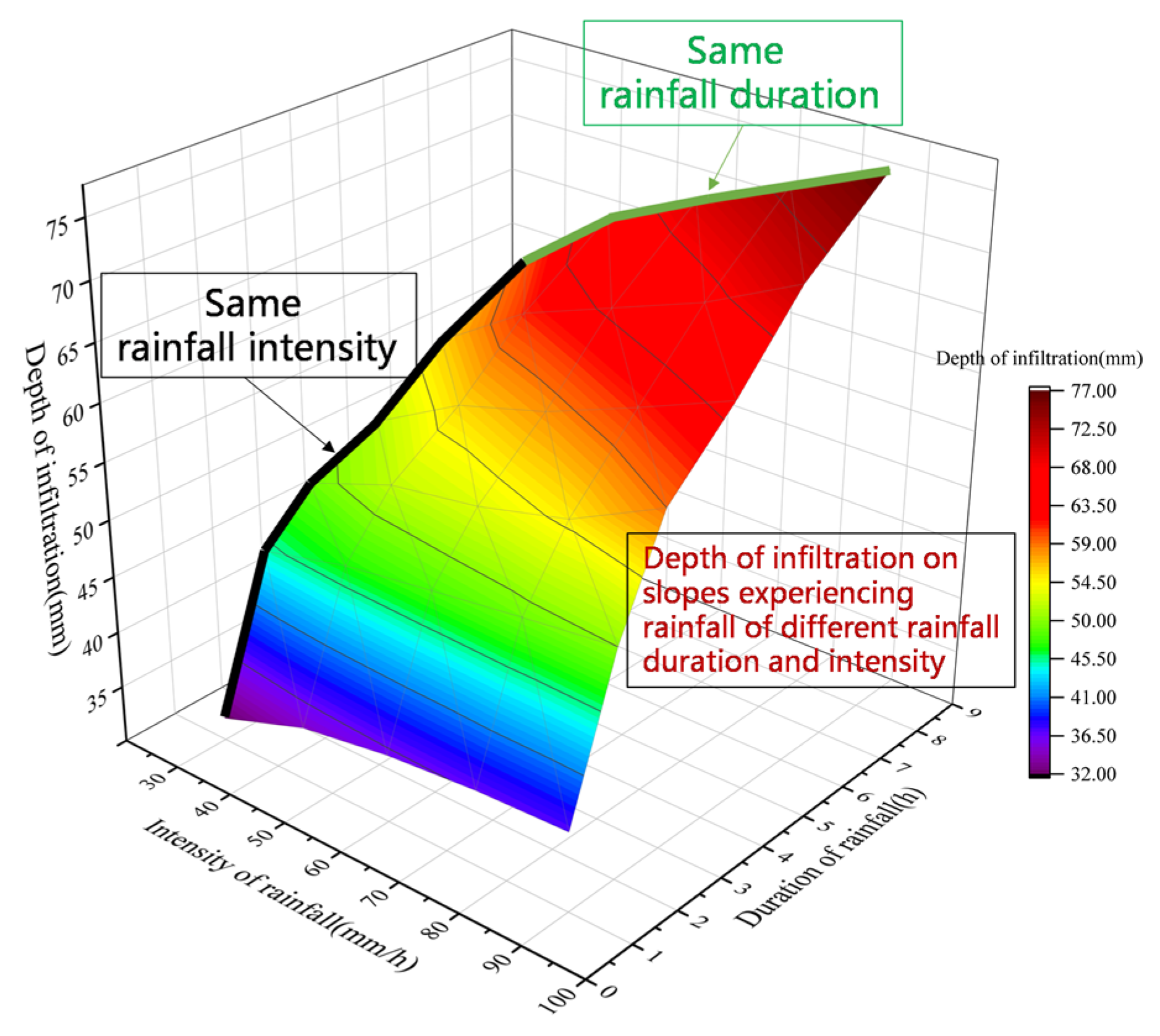
To examine the impact of rainfall intensity and duration on the infiltration of Xiashu loess slopes, an artificial rainfall simulation device was used to apply varying levels of rainfall. Figure 6 displays a 3D surface plot of the infiltration depth ranging from 32 mm to 77 mm. The plot is based on a 35° slope angle, a rainfall intensity ranging from 30 mm/h to 90 mm/h, and a rainfall duration ranging from 1 h to 8 h. It is evident that the depth of infiltration generally increases with the increase in both rainfall intensity and duration. The impact of rainfall with varying intensity and duration on the depth of infiltration is significant. However, as can be seen from the figure, the increase in rainfall duration is more significant for the increase in slope infiltration depth than the increase in rainfall intensity.

3.4. Impact Factors and Data Sources

Researchers have continuously analyzed the factors affecting the depth of slope infiltration, including soil particle structure, infiltration rate, rainfall, and slope morphology. However, analyzing intrinsic factors such as soil structure and infiltration rate is complicated, and obtaining real-time parameters inside the soil is difficult. On the other hand, analyzing slope morphology and rainfall is relatively straightforward and manageable. This paper analyzes the effect of rainfall intensity, rainfall duration, and slope angle on the depth of slope infiltration based on field tests. This study found that rainfall duration and intensity have a positive correlation with slope infiltration depth, while slope angle has a negative correlation. These factors have a significant impact on slope infiltration depth.

The data presented were obtained through artificial simulated rainfall tests and numerical simulations on a typical Xiashu loess slope in Jurong City. The analysis focused on the depth of slope infiltration under different rainfall conditions by applying rainfall of varying intensities and durations to the Xiashu loess slope in the test section. After the slope-cutting treatment, we analyzed infiltration on slopes with varying angles. The soil’s water content at various depths within the slope was used to determine the depth of infiltration.

This article obtained 72 sets of sample data, which were divided into training, validation, and prediction sets in a certain proportion.

Table 1. Partial test data.

Serial Number	Slope Angle/°	Rainfall Intensity/mm·h−1	Rainfall Duration/h	Infiltration Depth/cm
1	35	30	2	44
2	30	60	4.5	62
3	40	30	4.5	47
4	40	90	1	33
5	25	30	8	70
6	30	60	1	38
7	35	90	2	50
8	20	60	4.5	69
9	25	30	2	54
10	30	60	2	52

displays some of the test data.

4. Modeling and Validation

4.1. Multiple Nonlinear Regression Modeling and Solution Validation

Based on the previous section, it is evident that changes in rainfall intensity, duration, and slope angle significantly affect the infiltration results. These results can serve as an indicator for predicting the depth of slope infiltration using the multiple nonlinear regression model.

To analyze the nonlinear effect of each factor on the depth of slope infiltration, we used experimental data to establish a regression model in SPSS 22 software. The model included the three aforementioned factors as independent variables and the depth of infiltration as the dependent variable. This paper adopts the type I nonlinear mathematical model due to the complexity of the type II model, making it difficult to accurately determine its form. The model considers the interaction between the independent variables and linearizes the nonlinear term through substitution, converting the nonlinear problem into a linear problem for analysis and solution. Because the multivariate nonlinear regression model does not have a unique solution, this paper first analyzes a single factor and then considers the impact of all factors. After several trial calculations, the ENTER analysis method of regression analysis is used for linear regression to exclude terms with collinearity and obtain the mathematical expression of the regression model. The fitting results are as follows:

$$\begin{gathered} y=49.99-0.96\ast X_1+0.088\ast X_2+9.19\ast X_3+0.005\ast X_1^2 \\ -0.539\ast X_3^2-0.028\ast X_1\ast X_3+0.021\ast X_2\ast X_3, \end{gathered}$$

(11)

where $X_1$ is the slope angle; $X_2$ is the rainfall intensity; $X_3$ is the rainfall duration; and $y$ is the depth of infiltration.

The regression equation shows that rainfall duration has the greatest impact on infiltration depth, followed by slope angle and then rainfall intensity. Based on the regression equation, the slope infiltration depth can be estimated by rainfall duration, rainfall intensity, and slope angle, and the results of this study can also be applied to the assessment of landslide damage depth.

The equation analysis results of the regression model are shown in

Table 2. Equation analysis of regression models.

Project	Sum of Squares	Free Degree	Mean Square	F Value	p
Model	15,760.152	8	1970.019	250.308	0.000
Error	1008.650	63	16.010	-	-
Total	16,768.802	71	-	-	-

. ANOVA and significance tests give D − W = 2.669, indicating that the data satisfy the independence requirement. The significance test for the nonlinear mathematical model F resulted in F = 250.308, which is much larger than F_0.05(8,63) =2.79, with a p-value of 0.000, indicating that the model is statistically significant at the 0.05 test level. Therefore, it can be determined that the multivariate nonlinear regression equations are valid. At the same time, R² = 0.936, which is closer to 1. It indicates that the strong linear relationship between y and x in the equation accurately reflects the actual change pattern, and the fitting effectiveness of the nonlinear regression equation is superior.

The depth of slope infiltration was analyzed using the established multivariate nonlinear regression equation, which was validated through testing 10 additional sets of field data selected at random. The regression equation was used to calculate the slope infiltration depth by substituting the input parameters into Equation (11). The relative error was analyzed by comparing the calculated values with the test data, as presented in

Table 3. Nonlinear regression model test results.

Serial Number	Infiltration Depth Obtained from the Experiment/cm	Model Calculation of Infiltration Depth/cm	Error
1	50	54.11	8.22%
2	58	61.45	5.95%
3	34	36.35	6.92%
4	49	44.19	−9.82%
5	56	59.07	5.48%
6	71	68.58	−3.41%
7	36	39.14	8.73%
8	51	47.60	−6.67%
9	67	64.02	−4.44%
10	77	75.71	−1.68%

. Table 3 shows that the nonlinear regression model has a minimum relative error of 1.68%, a maximum relative error of 9.82%, and an average relative error of 6.13%. Therefore, this model is suitable for prediction.

4.2. PSO-BP Neural Network Modeling and Solution Validation

The information from 72 data sets was used to create a predictive model. Totals of 50 sets were used for training, 11 for validation, and 11 for testing. This means that 70% of the total data were used for training and 30% for testing and validation.

The PSO-BP neural network modeling process begins by importing the predicted data into Matlab R2018b. The data are then randomly disrupted and divided into training and test sets, followed by normalization. The neural network structure consists of three layers: three input nodes, one output node, and a hidden layer with three nodes. The number of hidden-layer nodes was determined through Matlab program training experiments using Equation (10). This structure was found to be optimal. The parameters of the particle swarm were set as follows: the population size was 10, the number of population iterations was set to 50, the learning factor was C₁ = C₂ = 4.494, and the particle flight speed range was [−1, 1]. The population iterates until optimal weights and thresholds are achieved, which are then assigned to the BP neural network for training. Training continues until preset conditions are met.

The neural network is trained using the Sigmoid function as the transfer function, and the lattice training function uses the BP algorithm training function Trainlm of L-M. The maximum number of lattice training times is 1000, the learning rate is 0.01, and the target error is 1 × 10⁻⁶. The number of nodes in the hidden layer and the target error is constantly varied and trained in different combinations. To demonstrate the impact of the particle swarm optimization algorithm, we compared the training results of the PSO-BP neural network with those of the BP neural network. 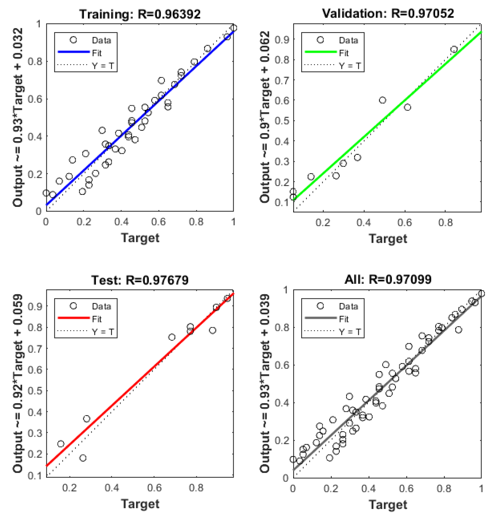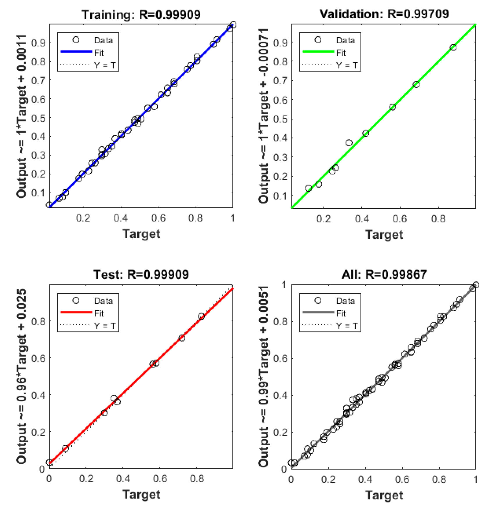Figure 7 and Figure 8 display the training results of the BP neural network and PSO-BP neural network, respectively. The figures show that the R² of the prediction model trained by the BP neural network is 0.943, while the R² of the prediction model trained by the PSO-BP neural network is 0.997. Compared to the multiple nonlinear regression model, both models are closer to 1 and have a better fitting effect.

The depth of infiltration of the Xiashu loess slope was calculated through iterative optimization and compared with the BP neural network using the PSO-BP neural network algorithm. Figure 9 and Figure 10 display the time and value of the optimal variance occurrence calculated by the BP neural network algorithm and the PSO-BP neural network algorithm for iterative optimization search. The BP neural network achieved its optimal mean square error of 0.0044243 after the 37th iteration, while the PSO-BP neural network achieved its optimal mean square error of 0.0003304 after the 19th iteration.

The accuracy of the model is measured using relative error and average relative error. To compare the predicted depth of infiltration with the actual depth of infiltration, other experimental data are randomly substituted into the PSO-BP neural network prediction model. The results of the relative error comparison are shown in

Table 4. PSO-BP neural network model test results.

Serial Number	Infiltration Depth Obtained from the Experiment/cm	Model Calculation of Infiltration Depth/cm	Error
1	72	73.12	1.56%
2	30	30.50	1.68%
3	54	54.32	0.59%
4	71	71.29	0.41%
5	56	55.69	−0.55%
6	83	83.09	0.10%
7	51	51.19	0.38%
8	38	37.77	−0.60%
9	49	49.17	0.36%
10	42	42.64	1.52%

. The figure illustrates that the PSO-BP neural network model has a minimum relative error of 0.10%, a maximum relative error of 1.68%, and an average relative error of 0.78%. The results indicate that the BP neural network model optimized by the particle swarm algorithm has achieved the expected goal with good prediction accuracy.

After obtaining prediction results from the multivariate nonlinear regression model and the PSO-BP neural network model, the experimental data were trained for prediction using the unoptimized BP neural network model. The prediction accuracies of the three models were then comprehensively compared.

Table 5. Comparison of three models.

Model	Multiple Nonlinear Regression	BP Neural Network	PSO-BP Neural Network
R2	0.936	0.943	0.997
MAPE	6.13%	5.29%	0.78%

displays the coefficients of determination (R²) and mean absolute percentage error (MAPE) for the three models. The formula for calculating the two is as follows:

$$R^2=1-\frac{\sum _{i=1}^n(y_i-\widehat{y_i}{)}^2}{\sum _{i=1}^n(y_i-\overline{y}{)}^2},$$

(12)

$$MAPE=\frac{1}{n}\sum _{i=1}^n\left[\frac{\left|\widehat{y_i}-y_i\right|}{\widehat{y_i}}\right]\times 100\%,$$

(13)

where $n$ is the predicted sample size, $y_i$ is the i-th measured value, $\widehat{y_i}$ is the i-th predicted value, and $\overline{y}$ is the sample mean.

Table 5 shows that all three models predicted the infiltration depth of the Xiashu loess slope well. However, the PSO-BP neural network model had the highest prediction accuracy compared to the other two models. The prediction accuracies of the three models were ranked as follows: PSO-BP neural network model > BP neural network model > multivariate nonlinear regression model.

To verify the applicability of the developed PSO-BP neural network model, it was applied to other slopes for infiltration prediction. The infiltration of other slopes in the area after experiencing natural rainfall was monitored during the test. The angle of the monitored slopes was about 33°, and the rainfall intensity and duration of natural rainfall were obtained by monitoring with a test instrument. The predicted values were compared with the real monitoring values using the established model, and the comparison results are shown in Figure 11. This confirms the validity of the model.

The PSO-BP neural network model predicts these three sets of data with an average relative error of 1.04%, which is higher than the other two models. This suggests that the model is applicable to other slopes in the region with good applicability.

5. Discussion

To mitigate the risks of landslides in the Xiashu loess during rainfall, it is essential to promptly evaluate the depth of infiltration of the Xiashu loess slopes. This assessment can roughly determine the extent of landslide damage and provide a new approach for the early warning and hazard assessment of landslides.

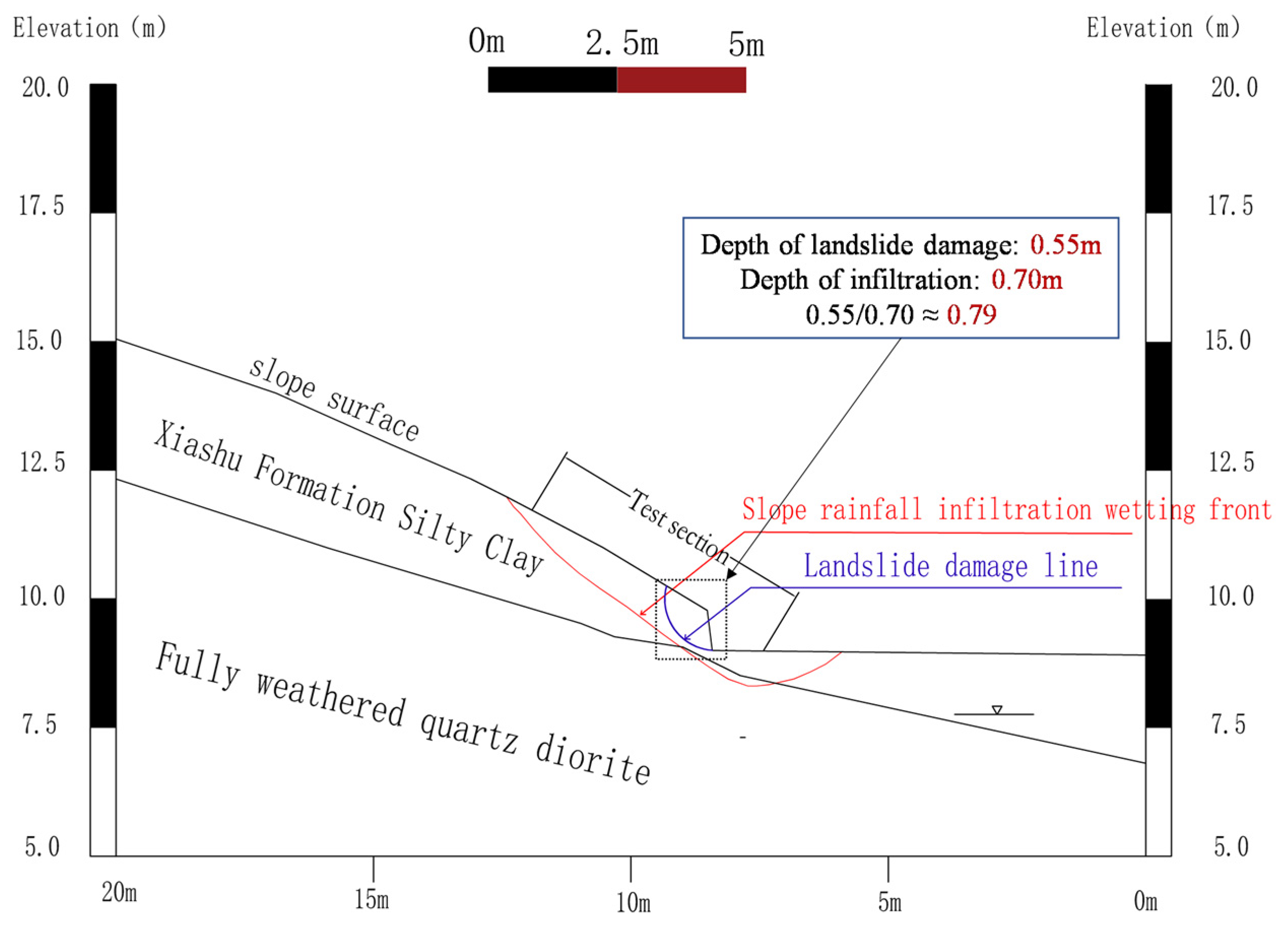
During the test, it was observed that the Xiashu loess slope suffered damage after 8 h of rainfall with a slope angle of 40° and a rainfall intensity of 90 mm/h. The diagram in Figure 12 shows the Xiashu loess landslide. The depth of the landslide is approximately 0.55 m, while the depth of infiltration is around 0.7 m. The depth of the landslide damage is about 0.8 times the depth of infiltration. Slopes undergo localized damage at the foot of the slope in the form of a circular arc, which is related to the fact that the depth of infiltration at the foot of the slope is greater than the depth of infiltration at the top of the slope and in the middle of the slope.

The Xiashu loess exhibits high water sensitivity, with its shear strength significantly impacted by water content. The angle of internal friction and cohesion decreases rapidly as the water content of the soil increases. During the rainfall process, the wetting front in the slope constantly moves forward, causing the thickness of the softened soil inside the slope to increase. This, in turn, leads to a dramatic decrease in the shear strength of the soil within the depth range of the wetting front, significantly increasing the probability of landslides occurring in the infiltration depth range of the soil. When the shear strength decreases to a certain threshold, it is not enough to support the force that causes the slope to slide. This leads to damage under the Xiashu loess slope, which is why most landslides occur at a certain depth of infiltration.

In a numerical simulation study of slope stability, it was found that the depth of infiltration has a significant effect on the slope stability coefficient. Particularly at the start of rainfall, an increase in infiltration depth results in a sharp decrease in the slope stability coefficient. The relationship between the depth of infiltration and the slope stability coefficient can be established, and the slope stability coefficient can be predicted based on the depth of infiltration.

As only one landslide occurred during the field test, it was not possible to establish a clear relationship between the depth of landslide damage and the depth of slope infiltration. Further tests can be conducted in future studies to explore this connection. The PSO-BP neural network-based slope infiltration depth prediction model presented in this paper offers a novel approach for determining the infiltration depth of Xiashu loess slopes. This lays the foundation for predicting the depth of Xiashu loess landslides and provides a new index for evaluating the stability of Xiashu loess slopes.

6. Conclusions

(1) This paper presents a prediction model for the infiltration depth of the Xiashu loess slope. The prediction data were obtained through field tests, using rainfall intensity, rainfall duration, and slope angle as input parameters, and infiltration depth as the output parameter. The particle swarm algorithm (PSO) was used to optimize the BP neural network, resulting in a model with improved convergence speed and generalization ability.

(2) The infiltration depth regression model for the Xiashu loess slope was expressed mathematically using the Class I nonlinear mathematical model. The model considered the interaction between independent variables, and the test results were predicted using the regression expression. The predicted results had an error range controlled within 10%, indicating that the nonlinear regression model was reasonable. This model provides a fast calculation method for determining the infiltration depth of the Xiashu loess slope.

(3) After comparing the slope infiltration depth prediction model established by the PSO-BP neural network with the multivariate nonlinear regression model and the traditional BP neural network model, it was found that all three methods have a good fitting effect and prediction ability. However, the PSO-BP neural network prediction model has a higher prediction accuracy than the other two models. The three models’ prediction accuracy is ranked as follows: PSO-BP neural network model > BP neural network model > multivariate nonlinear regression model. This ranking fully demonstrates the effectiveness of the PSO-BP neural network model in predicting the depth of infiltration of the Xiashu loess slope.

Due to the limitations of the test, the established prediction model only considered three factors: rainfall duration, rainfall intensity, and slope angle. To improve the model’s completeness, the effects of other factors should be further considered in subsequent tests.