The Application of Sand Transport with Cohesive Admixtures Model for Predicting Flushing Flows in Channels

Abstract

The feature of self-cleansing in sewer pipes is a standard requirement in the design of drainage systems, as sediments deposited on the channel bottom cause changes in channel geometric properties and in hydrodynamic parameters, including the friction caused by the cohesive forces of sediment fractions. Here, it is shown that the content of cohesive fractions significantly inhibits the transport of non-cohesive sediments. This paper presents an advanced calculation procedure for estimating flushing flows in channels. This procedure is based on innovative predictive models developed for non-cohesive and granulometrically heterogeneous sediment transport with additional cohesive fraction content to estimate the magnitude of increased flow necessary to ensure self-cleansing of channels. The computations according to the proposed procedure were carried out for a wide range of hydrodynamic conditions, two grain diameters, six cohesive (clay) fraction additive contents and two critical stress values. The trend lines of calculations were composed with the results of experimental studies in hydraulic flumes.

1. Introduction

Sediment transport processes in sewage systems are challenging for both engineers and researchers due to a number of reasons. Their complexity arises from the interaction between a variety of physical, chemical and biological processes, which often occur simultaneously. In sanitary, stormwater and combined sewer systems, sediments with a variety of cohesion can be encountered, ranging from completely non-cohesive, through partially cohesive to cohesive.

The definition of sewage sludge covers a wide range of particle sizes, from microscopic clay particles to larger gravel chunks. The cohesiveness of these sediments can be enhanced by a variety of admixtures, both inorganic and organic, including dust, silt and the metabolic products of microorganisms. Such heterogeneity of sediment material highlights the need for accurate predictive methods capable of accounting for these diverse properties in order to effectively manage wastewater systems [1,2,3].

The phenomenon of sedimentation in sewers occurs when flow velocities are too low to allow the pipes to self-clean, leading to the accumulation of deposits that can significantly reduce transport efficiency. Conversely, at higher flow velocities, erosion can occur, leading to a sudden increase in the concentration and transport of pollutants in the aquatic environment, affecting changes in the amount of pollutant transport [4,5,6].

1.1. Review of the Literature

Safari’s research extensively examines sediment transport in rigid boundary channels, focusing on the development of self-cleansing models for drainage systems. The researcher conducted experiments across various channel cross-sections to explore incipient motion and deposition, underscoring the significance of channel shape in self-cleansing design. A notable advancement was defining the optimum deposited bed thickness for sewer self-cleansing.

Different drainage system design methods are traditionally based on the assumption of non-sedimentation of sedimentary material, assuming minimum values of flow velocity or shear stress in the channel bed based on experience, without deeper theoretical justification [7,8,9,10,11,12,13].

These works are experience-based approaches which are generally limited by the range of experiments. The limitations of existing self-cleansing approaches are often based on the minimum values of flow velocity or shear stress required to initiate sediment movement. In a series of publications, [7,8,9,10,11,12,13] published the laboratory experimental results on initial sediment movement. The experiments were conducted in trapezoidal, rectangular, circular, U-shaped and smooth V-shaped channels using four different sand sizes. For shear stress, the dimensionless values proposed by Shields are usually used [14].

Due to the complexity of the phenomena occurring during the transport of sediments over non-cohesive, partially cohesive or fully cohesive bottoms, there is still an urgent need for theoretical solutions, the validity of which would not be limited by the range of measurements used to verify these solutions. Despite these advancements, gaps in the research remain. The subjective definition of sediment transport conditions, variations in experimental setups, and limited consideration of complex flow conditions pose challenges to the development of universally applicable self-cleaning models. Additionally, further research is needed to address the applicability of existing models across diverse environmental conditions and sediment types.

Zhang, Singh and Bengtsson’s [15] paper offers a comprehensive view of sediment transport dynamics in urban drainage systems, highlighting the importance of hydrodynamic modelling and its impact on water quality management. Their research provides an important contribution to the understanding of complex interactions between water flows and transported materials, which has direct implications for the design of more effective waste management systems. Morales and Knight [16] explore the effect of cohesive admixtures on the transport of non-cohesive sediments in open channels. Their research provides new experimental data and analyses that are key to the development of more accurate sediment transport models, particularly in the context of increasing the efficiency of flushing flows and preventing sedimentation of materials.

Kim and Sanders [17] present advanced modelling of sediment transport during floods using coupled hydrodynamic and sediment transport models. Their paper provides more accurate forecasting and planning, which is essential to protect infrastructure and the environment from the effects of extreme weather events. Gupta and Kumar [18] focus on numerical modelling of sediment transport under different flow conditions, which is crucial for forecasting and managing sediment in channels. Their paper shows how advanced modelling techniques can contribute to a better understanding of sediment transport processes and their impact on hydraulic infrastructure. Chen and Chiew [19] investigate the role of biofilms in sediment transport dynamics in sewer systems, which is a new direction in the study of interactions between biological and physical processes in sediment transport. Their paper points to the potential benefits of integrating biological processes into sludge transport modelling, which could lead to more sustainable solutions in waste management.

Rajaratnam and Ahmari [20] analyze the impact of urbanization on sediment transport in storm drains, highlighting the importance of managing runoff in the context of a changing urban landscape. Their field research provides valuable data that can contribute to better urban infrastructure planning aimed at minimizing the negative impact of urbanization on the aquatic environment.

The above literature review shows how significant progress has been made over the last several decades in the field of theoretical description of transport dynamics in urban drainage systems, highlighting the importance of hydrodynamic modelling and indicating, however, a growing need for more sophisticated predictive tools.

In the context of design challenges, the [21,22] standards define general objectives and functional requirements for drainage and sewerage systems, at the same time leaving the methodology for solving specific engineering problems to professionals.

The dynamics of sediments containing fine and coarse non-cohesive particles is the result of their transport, which is accompanied by mass and momentum exchange processes, leading to bed erosion and the formation of high-concentration suspensions and their settling in the bed substrate. There are numerous studies related to the dynamics of sediments transported and sorted in coastal regions and rivers, starting from [23] to [24,25,26,27] and [28,29] up to [30,31,32,33,34,35], which include both theoretical and experimental research. Works related to the transport of sediments were conducted in several directions. However, there is still a knowledge gap that concerns the theoretical studies on non-cohesive sediment transport without and especially with cohesive additions.

Modelling of non-cohesive and cohesive sediment transport should involve complex interactions between sediment particles, fluid dynamics and bed structure. Kaczmarek et al. [36] propose a multilayer model of sediment transport in steady flow over a bed with a moving sediment layer, focusing on non-cohesive sediments. The model takes into account different physical processes occurring at different distances from the solid bottom up to the water surface.

This model is dedicated to both wave conditions [36,37,38,39,40] and unidirectional flows [41,42]. More recently, the model has been extended to account for the contribution of cohesive fraction additions to the transport of non-cohesive granulometrically heterogeneous sediments [43].

Subsequently, the authors [42] extended the computational model to analyze the transport of granulometrically diverse sediment mixtures under steady flow conditions, with additional consideration of the role of the finest fraction.

The experimental studies [42,43,44] provided the data for the verification of accurate theoretical predictions. In all cases, i.e., for tests carried out in the hydraulic channel at the Institute of Hydro-Engineering (IHE) of the Polish Academy of Sciences (PAS) in Gdansk [42,43] and in the hydraulic channel in the University of Ghent, Belgium [44], high agreement of the calculation results with measurements was achieved within the double determination error.

In summary, the proposed sediment transport model, both without [41,42] and with cohesive admixtures [43], highlights the complexity of sediment dynamics. The introduction of cohesive forces presents additional factors that must be taken into account when predicting sediment transport rates, particularly highlighting the complex interaction between sediment fractions, water flow and bed morphology.

1.2. The Aim of the Study

This paper focuses on analyzing the complexity of sediment transport phenomena, highlighting that sewers’ self-cleansing efficiency is sensitive to sediment quantity and quality changes.

The aim of this study is to develop a computational procedure to effectively implement the results of modelling the above-mentioned transport of sediments with cohesive additives in engineering practice, in particular in the design and modernization of sewerage systems, in accordance with [21,22].

In the lack of specific prescriptive guidance, the proposed study, based on solid science, provides a key tool for engineers to design drainage systems that meet the highest standards of safety and efficiency, enabling the effective management of sedimentation risks and ensuring the continuity of the self-cleansing process.

This work seeks to bridge the gap between theoretical models and practical engineering applications by proposing a new computational procedure that implements these models effectively in sewer system design, aligning with the latest standards and addressing current shortcomings in design methodologies.

2. Materials and Methods

2.1. Summary on Modelling Transport of Sediments with and without Cohesive Additives

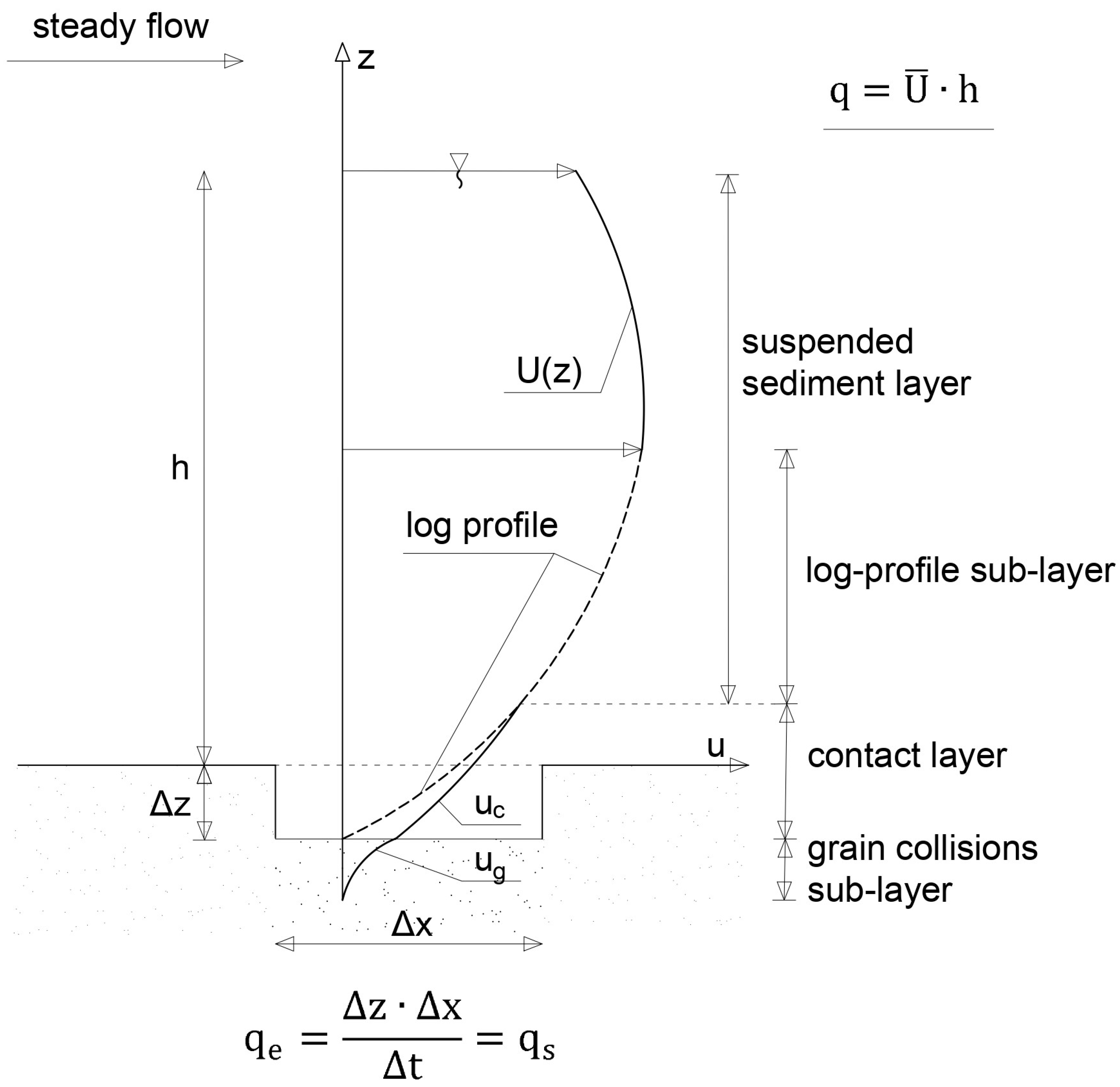
The proposed model is based on a multilayer approach that allows distinguishing between different physical processes occurring at different distances from the solid bottom (Figure 1). The proposed structure consists of several layers, including a dense layer (with a fixed Coulomb friction sub-layer and an upper mobile sub-layer dominated by grain collisions), a contact layer (where particle collisions and turbulent uplift interact in momentum exchange) and a suspended sediment zone. In the moving sub-layer of the dense layer, it is assumed that at all levels from the solid bottom, all sediment fractions move with equal velocity to the velocity of a mixture, which means that interactions between sediment fractions are very strong and, consequently, finer fractions are slowed down by coarser fractions. The model also takes into account the intensive sediment sorting in the process of grain dispersion in the contact layer and in the turbulent flow zone, which leads to sediment suspension. This ensures that sediment transport can be modelled accurately, taking into account various interactions between sediment fractions, at different levels from the solid bottom.

Therefore, a three-layer system with a lower, middle and upper zone was proposed, aiming to provide full, continuous velocity and sediment concentration profiles, from the solid bottom up to the free water table. In particular, a new vertical shear stress structure was proposed, characterized by its increase to a maximum value near the bottom and its decay at the bottom, i.e., at the upper boundary of a dense layer and its further decay at the bottom. Consequently, the contribution of each layer to the total transport varies for different hydrodynamic conditions described by the shear rate. Thus, when the flow near the bottom is fully mobilized, the contribution of the upper dense sub-layer and the contact layer to sediment transport is dominant, while their contribution is negligible under conditions close to the initial movement. Only grains located at the upper boundary, immobile in this case, of the entire dense layer are then transported in the bedload regime. The model is effective over a very wide range of grain mobility conditions, from initial movement to a fully mobilized bottom. The theoretical description has been verified with multiple data sets for different grain diameters and densities [38].

Zawisza et al. [42] further develop the model for sediment mixture transport in a steady flow, particularly focusing on the additional contribution of very fine non-cohesive fractions. These studies highlight the significant role of these fine fractions in the transport dynamics of coarser sediment in a sediment mixture. Interaction effects between different sediment fractions are key to understanding transport rates in poorly sorted, granulometrically heterogeneous mixtures.

Next, Zawisza et al. [43] extend the understanding of sediment transport by including cohesive admixtures in the analysis. He highlights how cohesive forces alter critical stress levels, delaying the initiation of grain movement and affecting the transport rate of sediment mixtures. The model assumes that the activated cohesive fraction, the magnitude of which is limited by the sediment porosity, spreads throughout the flow area without significantly affecting the transport rate of non-cohesive fractions.

Therefore, the presence of cohesive admixtures in the sediment increases critical shear stress for the initiation of sediment movement. Then, due to sediment transport after the time $\Delta t$, the erosion of the bed is created (Figure 1) and simultaneously the cohesive admixtures are released from the bottom of the thickness $\Delta z$ (Figure 1). Hence, after the time $\Delta t$ and erosion $\Delta z$, there is no change in the percentage of cohesive and non-cohesive sediments in the bottom layer below $\Delta z$. Further, for flow flushing processes it is advantageous to carry the cohesive material away instead of depositing it at the bottom.

In order to make it more clear how the model works, detailed flow charts for the calculation of sediment transport rates for sediments with and without cohesive admixtures are shown in Figure 2.

2.2. Computational Procedure for Flushing Flows

An arbitrary cross-sectional shape with a defined wetted perimeter $L_0$ is considered, in which non-cohesive sediments with cohesive additions up to approximately 30% of the content may be deposited (Figure 3). The 30% magnitude is due to the limitation of cohesive fraction admixtures to the sediment porosity. It is assumed that sediment deposition takes place over a certain section $L_0$ and, therefore, it is of interest to mobilize a layer of such width (Figure 3). As it is assumed that the cause of movement (sediment transport) is the shear stress ${\theta }_{\ast }^{\prime }$, it is of interest to mobilize this layer over this section. For this purpose, it is possible to assume $R_h=h$ and the wetted perimeter equal to the width of deposited layer $L_0=B$.

Taking into account the fact that sediment deposition at the bottom occurs as a result of inhibiting the transport of non-cohesive sediments by cohesive additives, a computational procedure is proposed for the designed channels by taking into account the necessary increase in flows.

The whole computational procedure (Figure 4) consists in finding such a new depth $h_k$, for which the friction acting on the bottom of width $B$ activates sediments with cohesive additives with a transport rate equal to the transport rate without cohesive additions for the original depth $h$. Under these conditions, there will be no sediment deposition, as it will be mobilized.

The calculation of the increase $\frac{Q_k}{Q}$ is carried out according to the algorithm shown in Figure 4.

The proposed computational procedure implementing sediment transport models with/without cohesion, which flow charts of numerical algorithms are shown in Figure 2.

It is worth noting that the use of the empirical Meyer-Peter and Muller (MPM) formula is proposed only for finding the magnitude of ${\gamma }_0^2$ and ${\gamma }_{0c}^2$, where the value of ${\tau }_0={\gamma }_0^2{\tau }_{\ast }^{\prime }$is the total shear stress at the upper boundary of dense layer in the case of non-cohesive sediments without cohesive additives, while ${\tau }_{0c}={\gamma }_{0c}^2{\tau }_{\ast }^{\prime }$ in the case of non-cohesive sediments with cohesive additives. In order to find the magnitude ${\gamma }_0^2$ (or ${\gamma }_{0c}^2$) the following equation is proposed:

$$\frac{q_g+q_c}{\sqrt{\left(s-1\right)g{d_r}^3}}=\Phi .$$

(1)

In which $\Phi$ is the dimensionless sediment transport in the mobile sub-layer of the dense layer and in the contact layer only. It is assumed that the magnitude $\Phi$ is equal to that determined using the MPM formula:

$$\Phi =8{\left({\theta }_{\ast }^{\prime }-{\theta }_{cr}\right)}^{1.5},$$

(2)

for sediments without cohesive additions, or

$$\Phi =8{\left({({\theta }_{\ast }^{\prime })}_{ef}-{\theta }_{cr}\right)}^{1.5},$$

(3)

for sediments with cohesive additives.

The dimensionless shields parameter ${\theta }_{\ast }^{\prime }$ is defined in a fallowing way:

$${\theta }_{\ast }^{\prime }=\frac{u_{f\ast }^{\prime 2}}{\left(s-1\right)g{d}_r},$$

(4)

where:

$$s=\frac{{\rho }_s}{{\rho }_w},$$

(5)

where: ${\rho }_s$—sediment density; ${\rho }_w$—water density; $g$—gravity.

The cohesive stresses ${\tau }_{coh}$ may be evaluated based on the shear velocity $u_{f\ast c}^{\prime }$ due to cohesion in a fallowing way:

$${\tau }_{coh}={\tau }_{\ast }^{\prime }-{\left({\tau }_{\ast }^{\prime }\right)}_{ef}=\rho {\left(u_{f\ast }^{\prime }\right)}^2-{\rho {\left(u_{f\ast }^{\prime }\right)}^2}_{ef},$$

(6)

where the effective shear velocity ${\left(u_{f\ast }^{\prime }\right)}_{ef}$ is equal to the value

$${\left(u_{f\ast }^{\prime }\right)}_{ef}=u_{f\ast }^{\prime }-u_{f\ast c}^{\prime }.$$

(7)

The shear velocity $u_{f\ast c}^{\prime }$ due to cohesion is proposed to be found based on the hydraulic experiments carried out in Gdansk in 2021 [42,43] and in the University of Ghent [44].

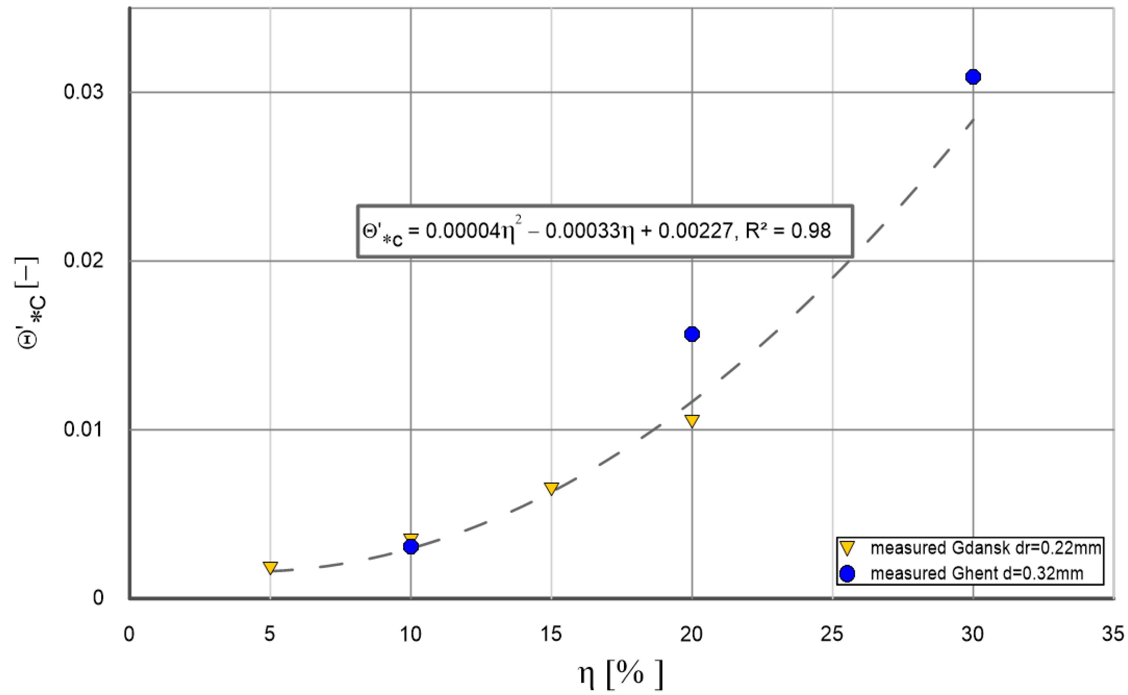
The shear velocity $u_{f\ast c}^{\prime }$ is evaluated from measured transport results plotted as a function of the measured shear velocity $u_{f\ast }^{\prime }$. The value $u_{f\ast c}^{\prime }$ for different clay contents was estimated as a value between the minimum measured value of $u_{f\ast }^{\prime }$ for total sediment transport $q_s=q_g+q_c+q_0$ equal to zero $(q_s=0)$ and the smallest measured value for $q_s\ne 0$. The dimensionless Shields parameter ${\theta }_{\ast \mathrm{c}}^{\prime }$ is defined as follows:

$${\theta }_{\ast \mathrm{c}}^{\prime }=\frac{u_{f\ast c}^{\prime 2}}{\left(s-1\right)g{d}_r}.$$

(8)

At this point it is worth recalling that, for sediments without cohesive admixtures ${\tau }_{coh}=0$ and $u_{f\ast c}^{\prime }=0$, while the onset of motion is determined by the dimensionless critical stresses ${\theta }_{cr}$, called the critical Shields parameter, the value of which is equal to about $0.05$ for sand placed smoothly on horizontal bed. Larger values ${\theta }_{cr}$ even on the order of $0.2-0.3$ can be measured for bottoms that are not perfectly flat. Further, it is worth noting that the inhibition of sediment transport takes place through the influence of the shear velocity $u_{f\ast c}^{\prime }$ due to cohesion on the measured shear velocity $u_{f\ast }^{\prime }$ (Figure 5). As a result, the critical shear stress for the initiation of sediment movement increases. This justifies the use of the MPM formula in the case of non-cohesive sediments with cohesive admixtures. Let us repeat, however, that this formula was used only to calculate the magnitude of shear stresses at the upper boundary of the dense layer. Sediment transport is calculated according to the algorithm shown in Figure 2.

Figure 5 shows the dependence of $\theta {\prime }_{\ast }c$ on the percentage of cohesive fractions $\eta \left[\%\right]$ for the results of Gdansk 2021 and Ghent 1998 experiments adopted for calculations.

The obtained best-fitting curve with a high coefficient of determination $R^2$ allows the calculation of the value ${{\theta }^{\prime }}_{\ast }c$ without the need to conduct additional hydraulic tests. Of course, it should be remembered that the obtained correlation curve applies only to cohesive clay materials, such as those used in experiments at the Institute of Hydro-Engineering (IHE) of the Polish Academy of Sciences (PAS) in Gdansk [42,43] and in the University of Ghent, Belgium [44]. In the case of other cohesive materials, additional hydraulic tests are required to determine the value of ${{\theta }^{\prime }}_{\ast }c$.

3. Discussion of the Results

Numerical calculations were carried out in accordance with the flow chart presented in Figure 2. Calculations were performed for a wide range of hydrodynamic conditions described by the dimensionless friction value ${\theta }_{\ast }^{\prime }$, starting from the value of ${\theta }_{\ast }^{\prime }=0.05 \left(0.21\right)$, up to the value of ${\theta }_{\ast }^{\prime }=2$. Numerical calculations of the transport value $q_s$, in the form of a dimensionless function ${\Phi }_s$, were carried out for two grain diameters, $d=0.22 \mathrm{mm}$ and $d=0.32 \mathrm{mm}$, and for six cohesive (clay) fraction additive contents, i.e., for $\mathrm{\eta }=0\%$, $\mathrm{\eta }=5\%$, $\mathrm{\eta }=10\%$, $\mathrm{\eta }=15\%$, $\mathrm{\eta }=20\%$ and $\mathrm{\eta }=30\%$. Moreover, calculations were carried out for four values of ${\theta }_{\ast c}^{\prime }$ (Figure 5) from Gdansk 2021 data and three values from Ghent 1998 data.

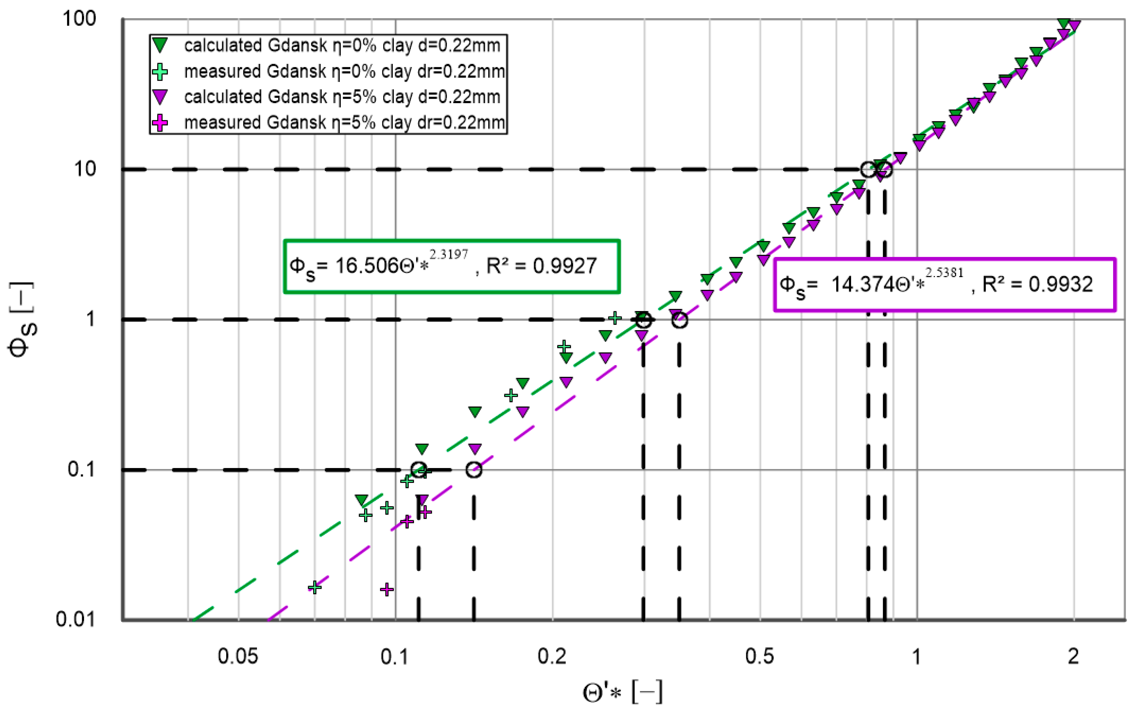
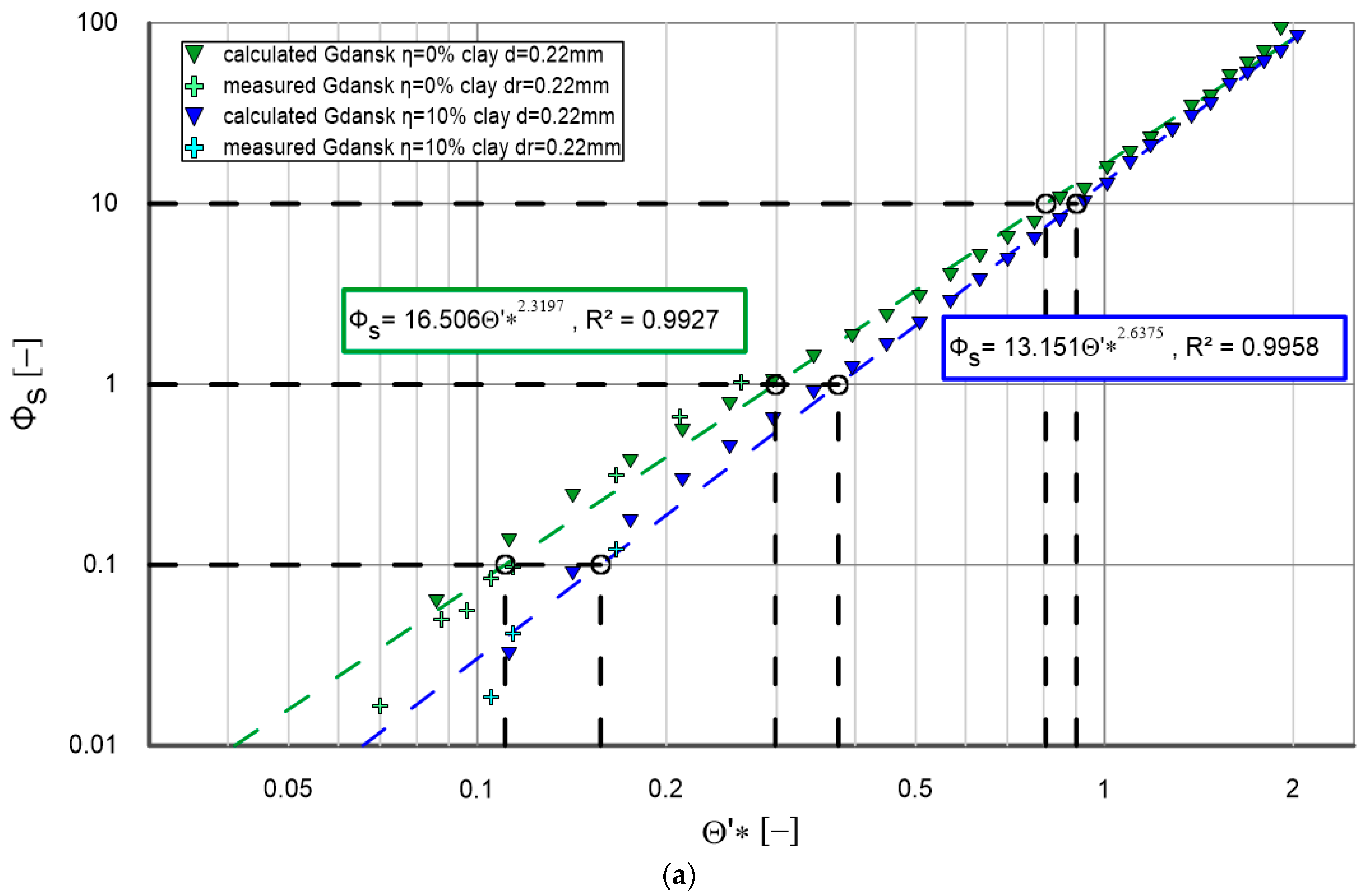
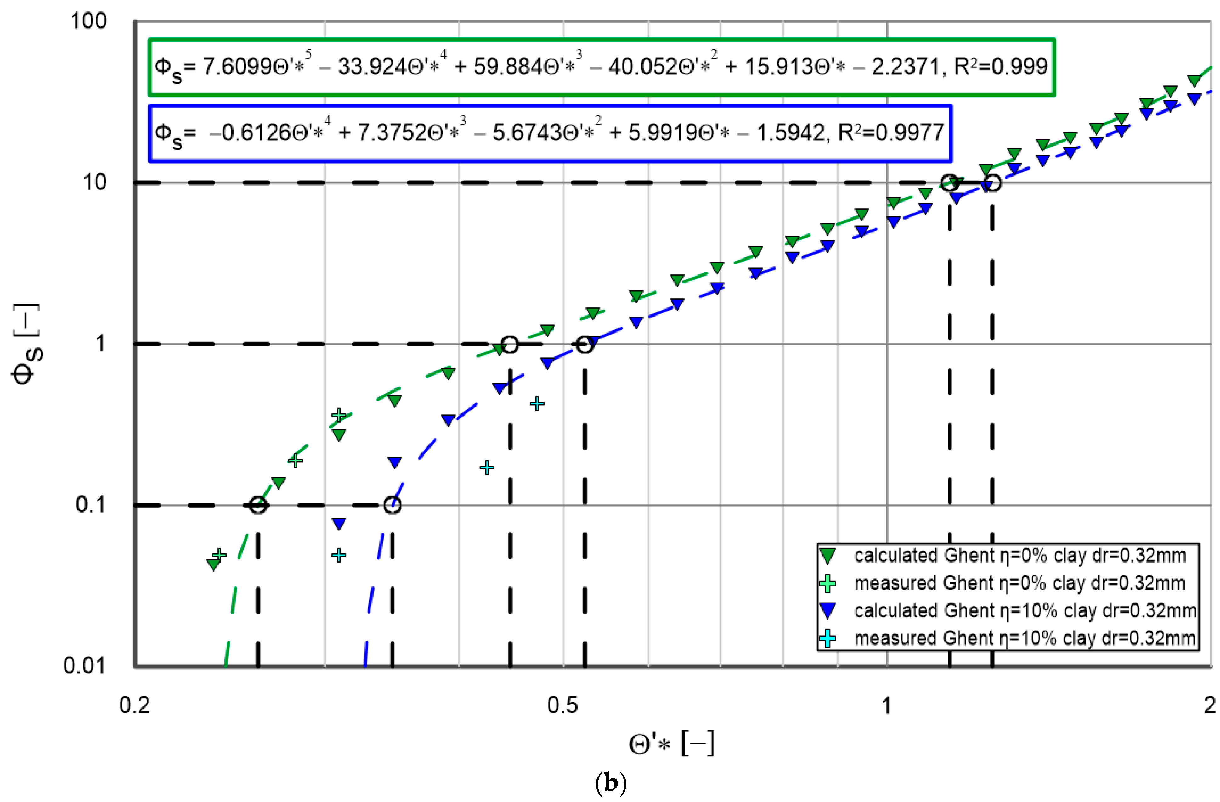
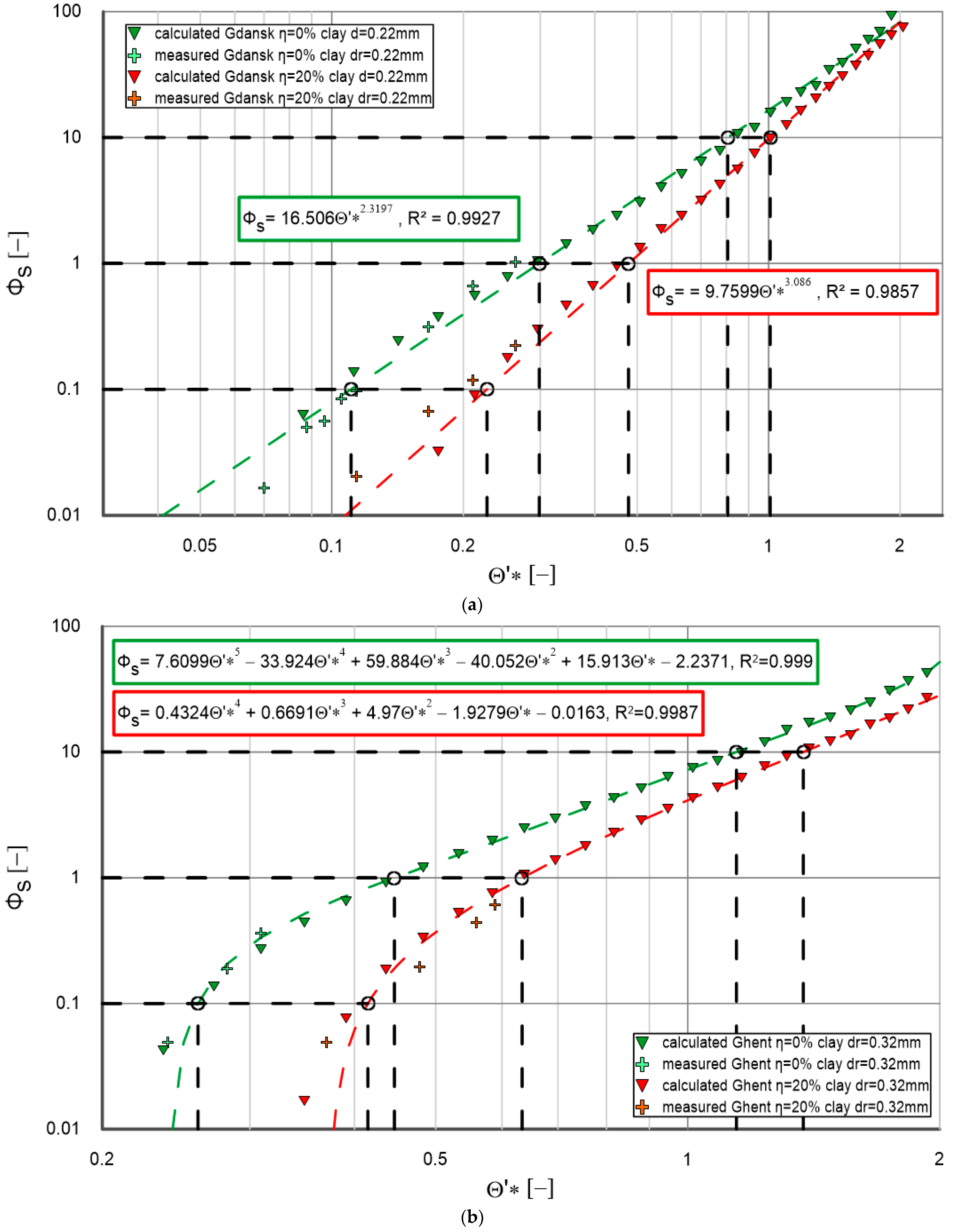
Figure 6, Figure 7, Figure 8, Figure 9 and Figure 10 show the results of numerical calculations of the dimensionless total transport quantities ${\Phi }_s$ depending on the dimensionless magnitude of friction ${\theta }_{\ast }^{\prime }$ for 0% and 5% (Figure 6), 0% and 10% (Figure 7), 0% and 15% (Figure 8), 0% and 20% (Figure 9) and 0% and 30% (Figure 10). The results of numerical calculations were then approximated by correlation curves with $R^2$ determination coefficients, obtaining a high fit value.

Following the determination of fitting degree of the correlation curves presented in Figure 6, Figure 7, Figure 8, Figure 9 and Figure 10 to the results of numerical calculations, in order to determine their reliability, they were compared with the results of experimental studies carried out in an IHE hydraulic flume in Gdansk in 2021 [43] and in a hydraulic flume in Ghent in 1998 [44]. A heterogeneous distribution with a diameter of diameter $d_r$ equal to median diameter $d_{50}=0.22 \mathrm{mm}$was used in the study in Gdansk, while a homogeneous distribution with a diameter of $d=0.32 \mathrm{mm}$was used in the hydraulic channel at Ghent University (Belgium). The studies in Gdansk and Ghent, although slightly different in scope, differed significantly in the magnitude of critical stress ${\theta }_{cr}$, from the magnitude ${\theta }_{cr}=0.05$ estimated on the basis of measurements in Gdansk to ${\theta }_{cr}=0.21$ in Ghent. The Gdansk study included transport measurements of sand with cohesive admixtures (clay) of 5%, 10%, 15% and 20%. The Ghent study included transport measurements of sand with cohesive admixtures (clay) of 10%, 20% and 30% (Figure 5).

As it was shown in [43], very good agreement between calculation results (according to the calculation procedure shown in Figure 2) and measurements were obtained within the experimental range. The agreement was achieved within plus/minus a factor 2 of the measurements. Here, very good agreement was obtained between the computational results represented by correlation curves and measurements, both for measurements made in Gdansk (Figure 6, Figure 7a, Figure 8 and Figure 9a) and Ghent (Figure 7b, Figure 9b and Figure 10).

Analyzing the presented figures in detail, several key trends and relationships can be observed:

• Calculated and measured data for different cohesive fraction contents (0%, 5%, 10%, 15%, 20% and 30%) are shown in each of the charts. The trend lines for calculated data are such that the $R^2$ determination coefficients for these lines are very high (typically above 0.99). A very high agreement obtained between measurements and calculations confirms that the results obtained provide a very good starting point for the calculation of flushing flows—according to the flow chart, Figure 4—for a granulometric composition with a diameter of $d_{50}$, for any value of ${\theta }_{cr}$ and for any value of ${\theta }_{\ast c}^{\prime }$ within the content of cohesive additives in the range from 0% to 30%.
• It can be concluded from the data that an increase in the cohesive fraction content results in a decrease in the amount of sediment transported. This is as expected, because cohesive materials tend to bind the grains, which hinders their mobilization and transport.
• For values of ${\theta }_{2.5}$ less than $0.5$ (weak and medium hydrodynamic conditions), the differences in transport between different cohesive fraction contents are more evident. Under stronger hydrodynamic conditions (${\theta }_{2.5}$ greater than $0.5$), the trend lines for different cohesive fraction contents are more similar, which indicates that at higher flows the influence of cohesive fraction contents on sediment transport decreases.
• It is worth noting that the correlation curves obtained based on numerical calculations in accordance with the calculation procedure shown in Figure 2, obtained for ${\theta }_{cr}=0.05$ (Figure 6, Figure 7a, Figure 8 and Figure 9a), differ significantly from those obtained for ${\theta }_{cr}=0.21$ (Figure 7b and Figure 9b) in the range of ${\theta }_{\ast }^{\prime }<0.8$, i.e., for small and medium hydrodynamic conditions. In the range of strong and very strong hydrodynamic conditions, i.e., up to ${\theta }_{\ast }^{\prime }\ge 0.8$, the differences between the calculations remain small.
• In conclusion, the analysis of graphs confirms that the effect of cohesive fractions on sediment transport is significant and depends on hydrodynamic conditions. In environments with weaker hydrodynamic conditions (lower values of ${\theta }_{2.5}$), the content of cohesive fractions plays a significant role in reducing sediment transport. In contrast, under stronger conditions, the differences in transport are smaller.

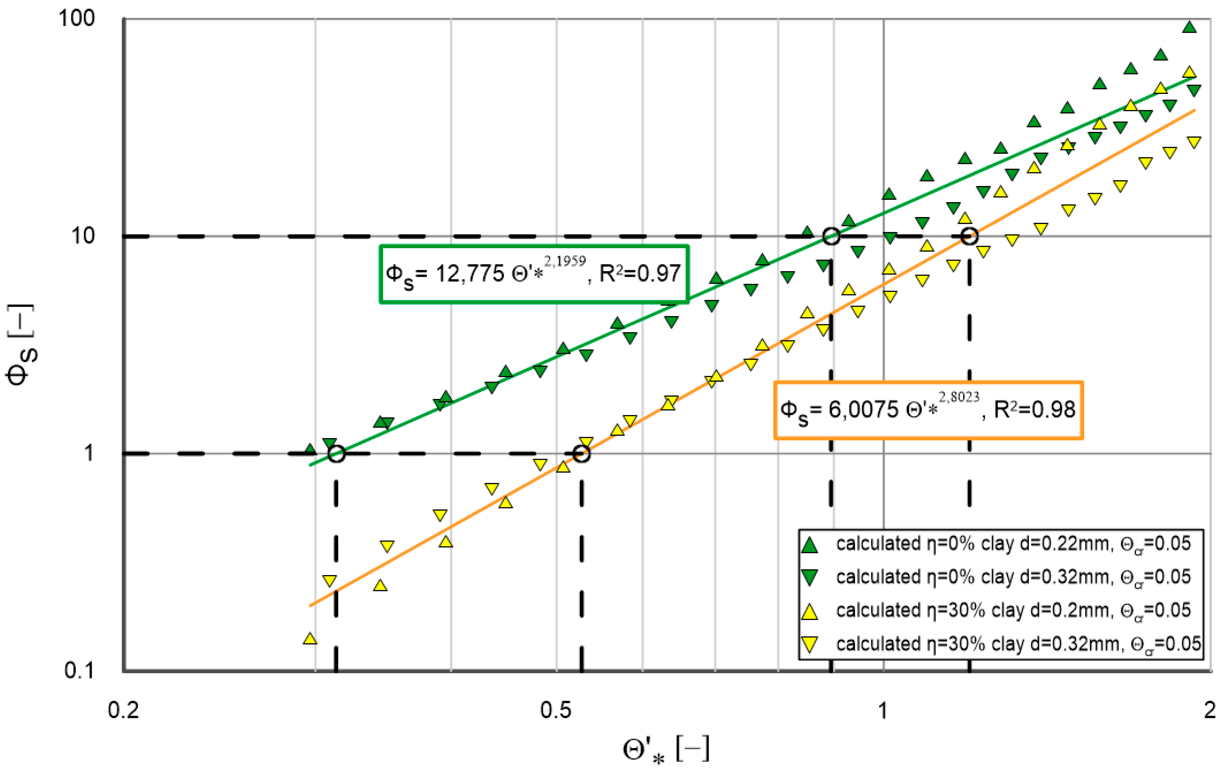
It is worth noting that the dimensionless function ${\Phi }_s$ allows comparisons of the calculated transport values $q_s$ for any grain size composition with any diameter $d_{50}$. Such calculations were carried out for two grain diameters, $d=0.22 \mathrm{mm}$ and $d=0.32 \mathrm{mm}$, in a wide range of hydraulic excitations ${\theta }_{\ast }^{\prime }$. The calculation results for the two diameters were approximated by one correlation curve with the determination coefficient $R^2$, obtaining a high fit value. Calculations were carried out for the content of cohesive fractions $\eta =30\%$ and for two values of critical stresses, i.e., for ${\theta }_{cr}=0.05$ (Figure 11) and for ${\theta }_{cr}=0.21$ (Figure 12). It seems that the results obtained are of great practical importance because they provide a modern “tool” for calculations for any grain size composition.

To sum up, it should be emphasized that the basis of the solution is the result of numerical calculations in accordance with the calculation procedure shown in Figure 2. The calculation results depend significantly on the input quantities, such as: the dimensionless value of the due to cohesion stress ${\theta }_{\ast c}^{\prime }$, the dimensionless value of the critical friction ${\theta }_{cr}$ and the grain diameter $d$. The calculation results can be approximated by any approximation curve, depending on the needs.

Figure 6, Figure 7, Figure 8, Figure 9, Figure 10, Figure 11 and Figure 12 show schematically the method of exploring—according to the scheme in Figure 4—the magnitudes of flushing flows $Q_k$, i.e., those for which the transport of non-cohesive sediments with cohesive additives is $q_{sck}=q_s$, for three selected flow rates $Q$, for which the dimensionless transport of non-cohesive sediments (without cohesive additives) is ${\Phi }_s$.

The calculation results of selected flushing flow rates depending on the percentage of cohesive fractions are compiled in

Table 1. Computational results of selected flushing flow rates as a function of cohesive fraction percentage.

Gdansk ${\mathit{\theta }}_{\mathit{c}\mathit{r}}\mathbf{=}\mathbf{\text{0.05}}$; d = 0.22 mm
${\Phi }_{\mathit{s}}$	$\raisebox{1ex}{${\mathit{Q}}_{\mathit{i}}$}\!\left/ \!\raisebox{-1ex}{$\mathit{Q}$}\right.=\raisebox{1ex}{${\mathit{h}}_i^{\raisebox{1ex}{$\mathbf{\text{5}}$}\!\left/ \!\raisebox{-1ex}{$\mathbf{\text{3}}$}\right.}$}\!\left/ \!\raisebox{-1ex}{${\mathit{h}}^{\raisebox{1ex}{$\mathbf{\text{5}}$}\!\left/ \!\raisebox{-1ex}{$\mathbf{\text{3}}$}\right.}$}\right.$
	$\raisebox{1ex}{${\mathit{Q}}_{\mathbf{\text{5}}\mathbf{\%}}$}\!\left/ \!\raisebox{-1ex}{${\mathit{Q}}_{\mathbf{\text{0}}\mathbf{\%}}$}\right.$	$\raisebox{1ex}{${\mathit{Q}}_{\mathbf{\text{10}}\mathbf{\%}}$}\!\left/ \!\raisebox{-1ex}{${\mathit{Q}}_{\mathbf{\text{0}}\mathbf{\%}}$}\right.$	$\raisebox{1ex}{${\mathit{Q}}_{\mathbf{\text{15}}\mathbf{\%}}$}\!\left/ \!\raisebox{-1ex}{${\mathit{Q}}_{\mathbf{\text{0}}\mathbf{\%}}$}\right.$	$\raisebox{1ex}{${\mathit{Q}}_{\mathbf{\text{20}}\mathbf{\%}}$}\!\left/ \!\raisebox{-1ex}{${\mathit{Q}}_{\mathbf{\text{0}}\mathbf{\%}}$}\right.$	$\raisebox{1ex}{${\mathit{Q}}_{\mathbf{\text{30}}\mathbf{\%}}$}\!\left/ \!\raisebox{-1ex}{${\mathit{Q}}_{\mathbf{\text{0}}\mathbf{\%}}$}\right.$
0.1	1.50	1.80	2.12	3.30
1.0	1.30	1.47	1.64	2.19
10.0	1.13	1.21	1.26	1.45
Ghent ${\mathit{\theta }}_{\mathit{c}\mathit{r}}=\mathbf{\text{0.21}}$; d = 0.32 mm
${\Phi }_{\mathit{s}}$	$\raisebox{1ex}{${\mathit{Q}}_{\mathit{i}}$}\!\left/ \!\raisebox{-1ex}{$\mathit{Q}$}\right.=\raisebox{1ex}{${\mathit{h}}_{\mathit{i}}^{\raisebox{1ex}{$\mathbf{\text{5}}$}\!\left/ \!\raisebox{-1ex}{$\mathbf{\text{3}}$}\right.}$}\!\left/ \!\raisebox{-1ex}{${\mathit{h}}^{\raisebox{1ex}{$\mathbf{\text{5}}$}\!\left/ \!\raisebox{-1ex}{$\mathbf{\text{3}}$}\right.}$}\right.$
	$\raisebox{1ex}{${\mathit{Q}}_{\mathbf{\text{5}}\mathbf{\%}}$}\!\left/ \!\raisebox{-1ex}{${\mathit{Q}}_{\mathbf{\text{0}}\mathbf{\%}}$}\right.$	$\raisebox{1ex}{${\mathit{Q}}_{\mathbf{\text{10}}\mathbf{\%}}$}\!\left/ \!\raisebox{-1ex}{${\mathit{Q}}_{\mathbf{\text{0}}\mathbf{\%}}$}\right.$	$\raisebox{1ex}{${\mathit{Q}}_{\mathbf{\text{15}}\mathbf{\%}}$}\!\left/ \!\raisebox{-1ex}{${\mathit{Q}}_{\mathbf{\text{0}}\mathbf{\%}}$}\right.$	$\raisebox{1ex}{${\mathit{Q}}_{\mathbf{\text{20}}\mathbf{\%}}$}\!\left/ \!\raisebox{-1ex}{${\mathit{Q}}_{\mathbf{\text{0}}\mathbf{\%}}$}\right.$	$\raisebox{1ex}{${\mathit{Q}}_{\mathbf{\text{30}}\mathbf{\%}}$}\!\left/ \!\raisebox{-1ex}{${\mathit{Q}}_{\mathbf{\text{0}}\mathbf{\%}}$}\right.$
0.1		1.61		2.18	2.58
1.0		1.30		1.79	2.13
10.0		1.16		1.36	1.47

and

Table 2. Computational results of selected flushing flow rates for any diameter d and for cohesive fraction percentage η = 30%.

${\theta }_{cr}=0.05$$; d=0.22 \mathrm{mm}$$\mathrm{and} d=0.32 \mathrm{mm}$$; {\theta }_{\ast c}^{\prime }=0.0125$
${\mathsf{\Phi }}_s$	$\raisebox{1ex}{$Q_i$}\!\left/ \!\raisebox{-1ex}{$Q$}\right.=\raisebox{1ex}{$h_i^{\raisebox{1ex}{$5$}\!\left/ \!\raisebox{-1ex}{$3$}\right.}$}\!\left/ \!\raisebox{-1ex}{$h^{\raisebox{1ex}{$5$}\!\left/ \!\raisebox{-1ex}{$3$}\right.}$}\right.$
	$\raisebox{1ex}{$Q_{30\%}$}\!\left/ \!\raisebox{-1ex}{$Q_{0\%}$}\right.$
1.0	2.38
10.0	1.63
${\theta }_{cr}=0.21$$; d=0.22 \mathrm{mm}$$\mathrm{and} d=0.32 \mathrm{mm}$$; {\theta }_{\ast c}^{\prime }=0.0125$
${\mathsf{\Phi }}_s$	$\raisebox{1ex}{$Q_i$}\!\left/ \!\raisebox{-1ex}{$Q$}\right.=\raisebox{1ex}{$h_i^{\raisebox{1ex}{$5$}\!\left/ \!\raisebox{-1ex}{$3$}\right.}$}\!\left/ \!\raisebox{-1ex}{$h^{\raisebox{1ex}{$5$}\!\left/ \!\raisebox{-1ex}{$3$}\right.}$}\right.$
	$\raisebox{1ex}{$Q_{30\%}$}\!\left/ \!\raisebox{-1ex}{$Q_{0\%}$}\right.$
0.1	2.75
1.0	2.13
10.0	1.59

.

The following conclusions can be drawn:

• It can be clearly seen that for each cohesive fraction content, as the hydrodynamic conditions defined by dimensionless friction ${\theta }_{\ast }^{\prime }$ increase, the increase in $\frac{Q_k}{Q}$ magnitude decreases.
• This increase, in turn, is the greatest for the smallest values of ${\theta }_{\ast }^{\prime }$ and reaches the largest values for $\eta =30\%$ cohesive fraction content.
• The computational procedure enables the calculation of flushing flow rates for any granulometric compositions with different $d_{50}$ diameters and any critical stress values.

4. Conclusions

The paper presents an advanced calculation procedure for estimating flushing flows in channels, based on innovative predictive models developed by [42,43]. These models are dedicated to non-cohesive sandy sediments and to sediments containing cohesive admixtures, respectively, taking into account the theoretical foundations of a three-layer model proposed by [41] for homogeneous sediments in a steady flow.

In order to determine the reliability of the proposed computational procedure, the calculation results were compared with a series of laboratory experiments conducted at the Institute of Hydro-Engineering of the Polish Academy of Sciences in Gdansk. The experimental studies included an analysis of the transport of sand with diameter $d_{50}=0.22 \mathrm{mm}$ and its fractions with cohesive admixtures (clay) in proportions of 5%, 10%, 15% and 20%. The experimental data by De Sutter [44] of Ghent University included an analysis of the transport of sand with diameter $d=0.32 \mathrm{mm}$ with cohesive admixtures (clay) in proportions of 10%, 20% and 30%. Analysis of the results showed a satisfactory correlation between the calculations represented by resultant trend lines for the transport of sand fractions in substrates with varying cohesive fractions and the experimental measurements.

A computational procedure has been developed for the estimation of flushing flow characteristics, depending on the cohesive admixture content of sediments. In particular, the procedure is dedicated to heterogeneous, non-cohesive sediments with a small content of cohesive fractions, under the assumption that their total volume does not exceed the substrate porosity.

The proposed computational procedure allows interpolation for different proportions of cohesive (clay) fractions affecting the partial cohesion of the sediment, assuming that the presence of these fractions increases the critical shear stress required to initiate sand movement, resulting in a reduction in sand transport efficiency.

It is assumed that once the cohesive fractions are released from the bottom, these fractions are dispersed in the water and no longer affect the further transport of sand fractions. It is shown that the content of cohesive fractions significantly inhibits the movement of sandy sediments, which has a direct impact on the transport rate of these fractions.

The calculation results of flushing flows according to the proposed computational procedure allow their magnitude to be estimated as a function of the percentage content of cohesive fractions, for any granulometric composition with a diameter of $d_{50}$ and for any value of critical stress, providing an important tool for engineers and scientists involved in modelling sedimentation and erosion processes in aquatic environments.

References

- Mehta, A.J.; Hayter, E.J.; Parker, W.R.; Krone, R.B.; Teeter, A.M. Cohesive sediment transport. I: Process description. J. Hydraul. Eng. 1991, 117, 1076–1093. [Google Scholar] [CrossRef]
- Banasiak, R.; Verhoeven, R.; De Sutter, R.; Tait, S. The erosion behavior of biologically active sewer sediment deposits: Observations from a laboratory study. Water Res. 2005, 39, 5221–5231. [Google Scholar] [CrossRef]
- El Ganaou, O.; Schaaff, E.; Boyer, P.; Amielh, M.; Anselmet, F.; Grenz, C. The deposition and erosion of cohesive sediments determined by a multi-class model. Estuar. Coast. Shelf Sci. 2004, 60, 457–475. [Google Scholar] [CrossRef]
- Ackers, P.; White, W.R.; Perkins, J.A.; Harrison, A.J.M. Sediment transport: New approach and analysis. J. Hydraul. Eng. 2001, 127, 935–948. [Google Scholar] [CrossRef]
- Butler, D.; May, R.P.; Ackers, J.C. Sediment transport in urban drainage systems. Urban Water 2003, 5, 235–243. [Google Scholar]
- Ashley, R.M.; Bertrand, N.; Hvitved-Jacobsen, T. Sewer sediment processes: Implications for sewer management. Water Sci. Technol. 2004, 49, 33–40. [Google Scholar]
- Safari, M.J.S.; Mohammadi, M.; Manafpour, M. Incipient motion and deposition of sediment in rigid boundary channels. In Proceedings of the 15th International Conference on Transport & Sedimentation of Solid Particles, Wroclaw, Poland, 6–9 September 2011. [Google Scholar]
- Safari, M.J.S.; Aksoy, H.; Mohammadi, M. Incipient deposition of sediment in rigid boundary open channels. Environ. Fluid Mech. 2015, 15, 1053–1068. [Google Scholar] [CrossRef]
- Safari, M.J.S. Self-Cleansing Drainage System Design by Incipient Motion and Incipient Deposition-Based Models. Ph.D. Thesis, Istanbul Technical University, Istanbul, Turkey, 2016. [Google Scholar]
- Safari, M.J.S.; Aksoy, H.; Unal, N.E.; Mohammadi, M. Non-deposition self-cleansing design criteria for drainage systems. J. Hydro-Environ. Res. 2017, 14, 76–84. [Google Scholar] [CrossRef]
- Safari, M.J.S.; Mohammadi, M.; Ab Ghani, A. Experimental studies of self-cleansing drainage system design: A review. J. Pipeline Syst. Eng. Pract. 2018, 9, 04018017. [Google Scholar] [CrossRef]
- Safari, M.S.; Shirzad, A. Self-cleansing design of sewers: Definition of the optimum deposited bed thickness. Water Environ. Res. 2019, 91, 407–416. [Google Scholar] [CrossRef]
- Safari, M.J.S.; Aksoy, H. Experimental analysis for self-cleansing open channel design. J. Hydraul. Res. 2021, 59, 500–511. [Google Scholar] [CrossRef]
- Meyer-Peter, E.; Müller, R. Formulas for bed-load transport. In Proceedings of the 2nd Meeting of the International Association for Hydraulic Structures Research, Delft, The Netherlands, 7 June 1948; International Association for Hydro-Environment Engineering and Research: Delft, The Netherlands, 1948. [Google Scholar]
- Zhang, L.; Singh, V.P.; Bengtsson, L. Comprehensive review of sediment transport dynamics in urban drainage systems. Adv. Water Resour. 2024, 143, 103659. [Google Scholar]
- Morales, R.; Knight, D.W. Effects of cohesive additives Ph.D., non-cohesive sediment transport in open channels. Water Sci. Technol. 2023, 67, 865–873. [Google Scholar]
- Kim, S.C.; Sanders, B.F. Advanced modelling of sediment transport in flood events using coupled hydrodynamic and sediment transport models. Water Resour. Res. 2023, 59, e2022WR031452. [Google Scholar]
- Gupta, H.; Kumar, P. Sediment transport under varying flow conditions: A numerical study. J. Hydrol. 2022, 596, 125785. [Google Scholar]
- Chen, Y.; Chiew, Y.M. Role of biofilms in sediment transport dynamics in sewer systems. Environ. Fluid Mech. 2023, 23, 521–537. [Google Scholar]
- Rajaratnam, N.; Ahmari, H. Impact of urbanization on sediment transport in stormwater runoff: A field study. J. Environ. Manag. 2024, 280, 111865. [Google Scholar]
- BS EN 752:2017; Drain and Sewer Systems Outside Buildings—Sewer System Management. British Standards Institution: London, UK, 2017.
- BS EN ISO 11295:2022; Plastics Piping Systems Used for the Rehabilitation of Pipelines. Classification and Overview of Strategic, Tactical and Operational Activities. ISO: London, UK, 2022.
- Mc Laren, P.; Bowles, D. The Effects of Sediment Transport on Grain-Size Distributions. J. Sediment. Res. 1985, 55, 457–470. [Google Scholar]
- Van Rijn, L.C. Longshore Sediment Transport, Report Z3054; Delft Hydraulics: Delft, The Netherlands, 2001. [Google Scholar]
- Van Rijn, L.C. Unified View of Sediment Transport by Currents and Waves. I: Initiation of Motion, Bed Roughness, and Bed-Load Transport. J. Hydraul. Eng. 2007, 133, 649–667. [Google Scholar] [CrossRef]
- Van Rijn, L.C. Unified View of Sediment Transport by Currents and Waves. II: Suspended Transport. J. Hydraul. Eng. 2007, 133, 668–689. [Google Scholar] [CrossRef]
- Van Rijn, L.C. Unified View of Sediment Transport by Currents and Waves. III: Graded Beds. J. Hydraul. Eng. 2007, 133, 761–775. [Google Scholar] [CrossRef]
- Van Rijn, L.C.; Walstra, D.J.R.; van Ormondt, M. Unified view of sediment transport by currents and waves. IV: Application of morpho dynamic model. J. Hydraul. Eng. 2007, 133, 776–793. [Google Scholar] [CrossRef]
- Van Rijn, L.C.; Grasmeijer, B.T.; Perk, L. Effect of channel deepening on tidal flow and sediment transport, part 1. Sandy channels. Ocean Dyn. 2018, 68, 1457–1479. [Google Scholar] [CrossRef]
- Egiazaroff, I.V. Calculation of nonuniform sediment concentrations. J. Hydraul. Div. 1965, 91, 225–247. [Google Scholar] [CrossRef]
- Gessler, J. Beginning and ceasing sediment motion. In River Mechanics; Shen, H.W., Ed.; Water Resources: Littleton, CO, USA, 1971; Chapter 7. [Google Scholar]
- Parker, G.; Klingeman, P.C. On why gravel bed streams are paved. Water Resour. Res. 1982, 18, 1409–1423. [Google Scholar] [CrossRef]
- Wilcock, P.R.; Mc Ardell, B.W. Surface-based fractional transport rates: Mobilization thresholds and partial transport of a sand-gravel sediment. Water Resour. Res. 1993, 29, 1297–1312. [Google Scholar] [CrossRef]
- Paola, C.; Seal, R. Grain Size Patchiness as a Cause of Selective Deposition and Downstream Fining. Water Resour. Res. 1995, 31, 1395–1407. [Google Scholar] [CrossRef]
- Sanford, L.P. Modelling a dynamically varying mixed sediment bed with erosion, deposition, bioturbation, consolidation, and armoring. Comput. Geosci. 2008, 34, 1263–1283. [Google Scholar] [CrossRef]
- Kaczmarek, L.M.; Sawczyński, S.; Biegowski, J. Hydrodynamic equilibrium for sediment transport and bed response to wave motion. Acta Geophys. 2015, 63, 486–513. [Google Scholar] [CrossRef]
- Kaczmarek, L.M.; Sawczyński, S.; Biegowski, J. An equilibrium transport formula for modeling sedimentation of dredged channels. Coast. Eng. J. 2017, 59, 1750015-1. [Google Scholar] [CrossRef]
- Kaczmarek, L.M.; Biegowski, J.; Sobczak, Ł. Modeling of Sediment Transport with a Mobile Mixed-Sand Bed in Wave Motion. J. Hydraul. Eng. 2022, 148, 04021054. [Google Scholar] [CrossRef]
- Radosz, I.; Zawisza, J.; Biegowski, J.; Paprota, M.; Majewski, D.; Kaczmarek, L.M. An Experimental Study on Progressive and Reverse Fluxes of Sediments with Fine Fractions in Wave Motion. Water 2022, 14, 2397. [Google Scholar] [CrossRef]
- Radosz, I.; Zawisza, J.; Biegowski, J.; Paprota, M.; Majewski, D.; Kaczmarek, L.M. An Experimental Study on Progressive and Reverse Fluxes of Sediments with Fine Fractions in the Wave Motion over Sloped Bed. Water 2023, 15, 125. [Google Scholar] [CrossRef]
- Kaczmarek, L.M.; Biegowski, J.; Sobczak, Ł. Modeling of Sediment Transport in Steady Flow over Mobile Granular Bed. J. Hydraul. Eng. 2019, 145, 04019009. [Google Scholar] [CrossRef]
- Zawisza, J.; Radosz, I.; Biegowski, J.; Kaczmarek, L.M. Transport of Sediment Mixtures in Steady Flow with an Extra Contribution of Their Finest Fractions: Laboratory Tests and Modeling. Water 2023, 15, 832. [Google Scholar] [CrossRef]
- Zawisza, J.; Radosz, I.; Biegowski, J.; Kaczmarek, L.M. Sand Transport with Cohesive Admixtures…—Laboratory Tests and Modeling. Water 2023, 15, 804. [Google Scholar] [CrossRef]
- De Sutter, R.; Huygens, M.; Verhoeven, R. Flume experiments of sediment transport in unsteady flow. In Transactions on Engineering Sciences; WIT: Cambridge, MA, USA, 1998; Volume 18, ISSN 1743-3533. [Google Scholar]
Figure 1.
Vertical structure of sediment transport and the layer of erosion.
Figure 2.
Flow charts of numerical algorithms for calculations of sediment transport with/without cohesion by model [44] and [42,43], respectively; whereby: —the skin shear stress at the top of the contact layer; —content of grains with diameter ; —representative diameter in grain collision sub-layer; , —the shear stress at the top of grain collision sub-layer; —without cohesion; —with cohesion; —thickness of grain collision sub-layer; —the shear velocity due to cohesion; —number of fraction; —water depth; —critical Shields parameter; MPM formula—Meyer-Peter and Muller formula 1948 [14].
Figure 3.
Graphical representation of the assumption in the calculation of , .
Figure 4.
Flow charts of numerical algorithms for calculations of flushing flows where: —is Maning’s roughness , —slope of the bottom ; Kaczmarek et al. 2019 [41]; Zawisza et al. 2023a [42]; Zawisza et al. 2023b [43].
Figure 5.
Dependence on for the results of experiments Gdansk 2021 and Ghent 1998 adopted for calculations.
Figure 6.
Dependence on for —Gdansk 2021 data; ; 0.0025.
Figure 7.
(a) Dependence on for —Gdansk 2021 data; ; 0.0035. (b) Dependence on for —Ghent 1998 data; ; .
Figure 8.
Dependence on for —Gdansk 2021 data; ; .
Figure 9.
(a) Dependence on for —Gdansk 2021 data; ; . (b) Dependence on for —Ghent 1998 data; ; .
Figure 10.
Dependence on for —Ghent 1998 data; ; .
Figure 11.
Dependence on for ; ; .
Figure 12.