
Recent Issues and Challenges in the Study of Inland Waters
by
 , , , and
Ryszard Staniszewski
1,*,
Beata Messyasz
2,
Piotr Dąbrowski
3,
Pawel Burdziakowski
4 and
and
Marcin Spychała
5 1
Department of Ecology and Environmental Protection, Poznań University of Life Sciences, Piątkowska 94 C, 60-649 Poznań, Poland
2
Department of Hydrobiology, Institute of Environmental Biology, Faculty of Biology, Adam Mickiewicz University in Poznan, Uniwersytetu Poznanskiego 6, 61-614 Poznań, Poland
3
Department of Environmental Management, Institute of Environmental Engineering, Warsaw University of Life Sciences, Nowoursynowska 159, 02-787 Warsaw, Poland
4
Department of Geodesy, Faculty of Civil and Environmental Engineering, Gdansk University of Technology, Narutowicza 11-12, 80-233 Gdansk, Poland
5
Department of Hydraulic and Sanitary Engineering, Poznań University of Life Sciences, Piątkowska 94A, 60-649 Poznań, Poland
*
Author to whom correspondence should be addressed.
Water 2024, 16(9), 1216; https://doi.org/10.3390/w16091216
Submission received: 1 April 2024
/
Revised: 19 April 2024
/
Accepted: 22 April 2024
/
Published: 24 April 2024
(This article belongs to the Special Issue Impacts of Climate Change and Anthropogenic Pressure on Freshwater Ecosystems)
Abstract
:This paper addresses several important problems and methods related to studies of inland waters based on the existing scientific literature. The use of UAVs in freshwater monitoring is described, including recent contact and non-contact solutions. Due to a decline in biological diversity in many parts of the globe, the main threats are described together with a modern method for algae and cyanobacteria monitoring utilizing chlorophyll a fluorescence. Observed disturbances in the functioning of river biocenoses related to mine waters’ discharge, causing changes in the physico-chemical parameters of waters and sediments, give rise to the need to develop more accurate methods for the assessment of this phenomenon. Important problems occurring in the context of microplastic detection, including the lack of unification, standardization and repeatability of the methods used, were described. In conclusion, accurate results in the monitoring of water quality parameters of inland waters can be achieved by combining modern methods and using non-contact solutions.
1. Introduction
Aquatic ecosystems, encompassing oceans, seas, rivers, lakes, and wetlands, are the habitats for an immense array of biodiversity crucial for their functioning. Understanding the complexities of biodiversity in aquatic environments is essential for effective conservation and sustainable management practices [1,2,3,4]. Aquatic ecosystems, with their water and sediment characteristics, support a high diversity of life forms, from microscopic plankton to macrophytes, macrozoobenthos and fish, playing important roles in global biogeochemical cycles and providing essential ecosystem services to humankind [5,6,7]. Observed changes in the functioning of aquatic ecosystems raise awareness of the need to undertake in-depth scientific analysis and practical actions, that could help reduce the negative effects of anthropopression [8]. Thus, increasing pressure on waters has been studied by many authors, tackling this with a wide range of scientific topics, modern research methods and considering possible solutions [9,10,11,12,13]. The situation is additionally complicated due to water scarcity in many regions of the World and conflicts for water resources inside countries (e.g., herders and farmers in Nigeria) or difficult relations between countries (e.g., Jordan River and countries along the Nile River) [14,15,16]. As this issue is very tough to solve, Wheeler and Hussein [17] have called for international studies on transboundary water problems on the basis of mutual understanding and empathy.
The presented paper focuses on several of the most important scientific and methodological aspects of water monitoring with respect to the observed problems. It discusses the potential and maybe not fully utilized capabilities of different methods and existing gaps in knowledge and practice, which could be overcome in the near future. For instance, the UAVs are still more popular and play an important role in different areas of life, but their use in aquatic studies is still in its initial state, despite obvious potential in water monitoring [18]. In the case of observed invasions of aquatic plant species [19], the use of drones could be helpful in the early detection of problems by visual inspection and using equipment for the analyses of chemical and biological parameters (e.g., fluorescens), thus helping in maintaining biological diversity [20]. In studies of the pressure of mining on inland waters, including its impact on biological features, brown coal mine waters were not sufficiently surveyed in recent decades. It is worth knowing that problems with water quality can be present also after mine closures [21]. Another very urgent topic is the presence of microplastic in waters, but surprisingly, the definition, sampling procedures and categorization for plastic are still not unified, causing problems with understanding between scientists [22].
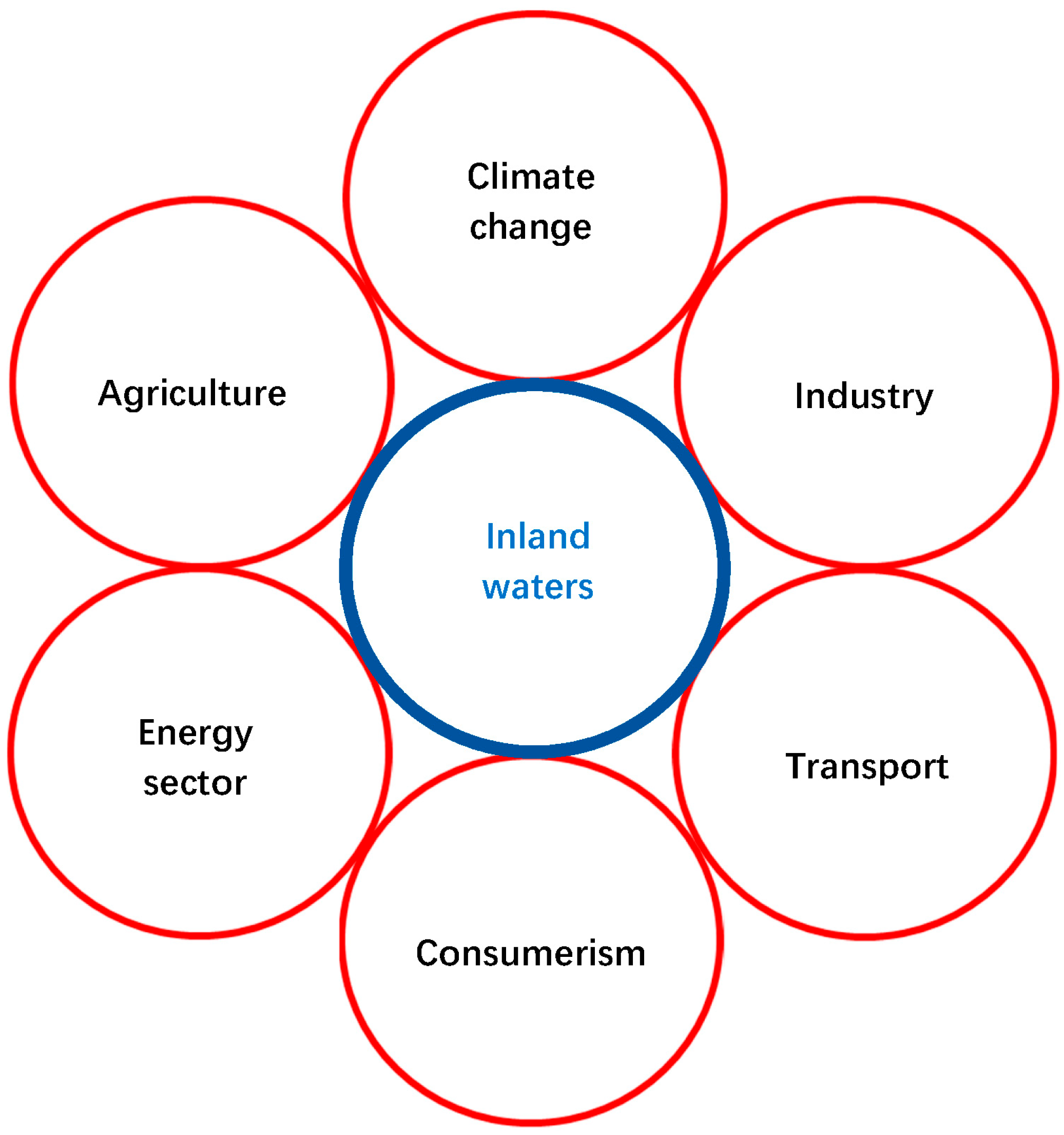
In our review, a wide range of recent scientific works on the use of UAVs (Unmanned Aerial Vehicles) in aquatic ecosystem monitoring is presented since it is a method which is helpful in the monitoring of all kind of pressures (Figure 1). The importance of biodiversity issues and recent studies on algae, both useful in the evaluation of industrial and agricultural pressures, is presented. The less studied impact of mine water (industry) on river ecosystems (i.e., aquatic plants) and the pressing issue of microplastics (due to consumerism and industry) in water are also explained.
2. Unmanned Aerial Vehicles in Inland Water Analyses
The UAVs of various types and sizes are now very well adapted to carry different types of functional payloads. A functional payload, performs a well-defined task at the location where it was delivered by the UAV, so the type of payload will determine the usage tactics of a particular type of UAV. For water quality measurements, we can divide functional payloads into sensor payloads, i.e., those provided for the study of physico-chemical parameters, and those in water sampling devices. We can further divide sensory devices into non-contact and contact sensors. The first group includes various types of remote sensing devices, such as multispectral cameras, hyperspectral cameras, visible light cameras, thermal imaging cameras and laser scanners (including bathymetric). The group of contact devices includes sensors for measuring physical and chemical parameters of water, which are submerged at a selected position in the water body. UAVs also allow water samples to be taken from the selected body of water and transferred for further analysis in the laboratory. The UAV water quality measurement solution is, therefore, divided into three main solutions: those based on non-contact (remote sensing) sensors, contact measurement devices and sample collection solutions. Each of these solutions is based on a flying platform, multi-rotor or airframe, which delivers the sensor or sampling device to the measurement site. A common feature of all solutions, resulting directly from the use of the UAV as a platform, is that the functional payload is safely delivered to the selected measurement site, the position of the measurement is accurately determined by the UAV’s navigation system, the flight itself and the execution of the navigation task by the UAV can be precisely programmed, the cost of using the UAV is low and the measurement system itself can be deployed quickly at the measurement site. These common features make the UAV an excellent platform for carrying sensors or samples, especially for small water bodies, which in the general case do not exceed the maximum flight range of the aerial platform in terms of their size.
2.1. Non-Contact Solution
This group includes all UAV-related work that is based on remote sensing data processing. The unquestionable advantage of these measurements is that there is no contact with the surveyed object during the measurement, which does not disturb the object, and the measurement itself is performed over a certain area. Remote sensing measurements made from UAVs are limited to only a certain range of the electromagnetic spectrum, which is somewhat smaller compared to satellite measurements. Due to the limited maximum mass of the functional payload, sensors designed and installed on UAVs are typically low in mass and are equipped with small sensor chips. This naturally results in them having slightly lower technical and accuracy capabilities than those installed, for example, on satellites. An important factor is that UAV data can be provided at a high time resolution, more frequently than satellite measurements and with a higher spatial resolution (smaller ground pixel). Remote sensing from UAVs is currently mainly used to estimate water quality parameters such as total suspended solids (TSS) [23,24,25,26,27], turbidity (TUB) [28,29,30], chlorophyll a (CHL-A) levels [31,32,33,34,35] and phycocyanin (PS) [36,37,38,39,40], transparency [41,42,43], total nitrogen [41,44,45,46,47,48], total phosphorus [49,50,51,52], algae [53,54,55], aquatic vegetation [56,57,58,59,60], siltation of reservoirs and rivers [61,62], urban black and smelly water bodies [63,64,65,66] and microorganisms in water [9,67,68,69,70]. The very type of remote sensing sensor provided for the measurement of water parameters is also not different from the solutions adopted in other fields of remote sensing with UAVs such as precision agriculture. They are the same universal sensors and many calculation methods are adapted to this task directly from other remote sensing fields. In other words, UAVs are not being specifically adapted for the use of remote sensing cameras to study water parameters, they are mainly standard solutions. Significant differences are only observed in data processing techniques, the calculation of results and the spatial resolution of data. This work [71] compares satellite data and a solution based on a UAV and a multispectral camera. In this work, the UAV was used to measure chlorophyll a as a quantitative descriptor of the phytoplankton biomass and trophic level. As the results show here, there is moderately good agreement between the three sensors (two satellites and one UAV) at different spatial resolutions (10 m, 30 m and 8 cm), indicating a high potential for the development of a multi-platform and multi-sensor approach to monitor the eutrophication of small reservoirs. It is worth noting here the significant potential of the high spatial resolution achieved from UAVs (8 cm), which, for small reservoirs, makes it possible to acquire data with a very high spatial resolution. Remote sensing from UAVs mainly uses four types of spectral cameras, which can be subdivided according to the method of data acquisition into: point scanning (or whiskbroom), line scanning (or pushbroom), plan scanning and single shot [72]. Multispectral cameras, offer up to approximately 10 spectral channels in the 400–1100 nm range with a width of up to 40 nm (e.g., Altum PT, RedEdge-P and RedEdge-P Dual of AgEagle Aerial Systems Inc., Raleigh, NC, USA). Hyperspectral cameras offer spectral ranges from 350 nm (CHAI V-640, Brandywine Photonics, West Chester, PA, USA) to even 2500 nm (SWIR-384, HySpex, Oslo, Norway) with an excellent spectral resolution as low as 1.3 nm (Pika XC, Resonon Inc., Bozeman, MT, USA). Such cameras allow for much more accurate analyses of the electromagnetic spectrum to be made.
In this paper [73], data were acquired from a small UAV equipped with a MicaSense RedEdge (MicaSense Inc., Seattle, WA, USA) multispectral camera. This is a small camera with five spectral channels and the difficulty in processing multispectral data from the UAV is precisely due to its relatively small spectral range. Here, the researchers presented an improved matching pixel-by-pixel (IMP-MPP) algorithm that successfully derived suspended solids and turbidity indices in a selected region of measurements based on these data. In contrast to this solution is the work of Lu et al. [74], where measurement data were collected with a hyperspectral camera (Headwall NANO-Hyperspec manufactured by Headwall Photonics Inc., Bolton, MA, USA) integrated with a UAV. This camera also operated in the same spectral range, but offered data with a spectral resolution of 6.0 nm, resulting in 100 spectral channels. An innovative solution using a hyperspectral sensor for CHL-A measurements is presented in paper [67]. Here, a hyperspectral sensor with a broad spectrum of 400–900 nm was placed on a UAV with a spectral channel every 5 nm, based on an acousto-optic tunable filter (AOTF) sensor. Solutions based on a visible light camera have also been successfully used to survey water bodies. In the work by [75], just such a small camera integrated with a UAV was used, where a method for assessing the concentration of tracer dyes placed in the surveyed water body was demonstrated. As it turns out, the small camera and the developed method of data filtering allows one to assess the concentration in the study area with high accuracy. This work also shows the important difference between the point-sampling method and the spatial measurement using a camera. In this way, data are available for an area rather than a point, allowing complex analyses related to dye dispersion to be made. Similar solutions are also presented in papers [76,77,78,79].
2.2. Contact Solutions
This group includes all UAV work which is based on sensors being delivered to the measurement site and immersed in the reservoir being surveyed. The undoubted advantage of this type of measurement is that the result (sensor reading) is obtained quickly and precisely at the selected location, unfortunately, rather point-like. In situ sensor measurements are precise, but are limited only to the values that the sensor registers. Importantly, such sensors are not standardized for UAV operation, so such devices are proprietary solutions. Researchers using standard sensors have adapted them to remotely record and transmit data to the UAV base station. Such solutions are based on using the 912 MHz radio frequency. In solutions of this type, standard sensors for determining water quality, e.g., pH, temperature, turbidity, dissolved oxygen (DO) and carbon dioxide, are integrated mechanically on the flying platform. The sensors are connected to a microcontroller on board the UAV, their readings transmitted to a ground station via the UAV’s telemetry channel. In this way, data are read out in real time [80]. In paper [81], the authors presented a small hexacopter that was equipped with a dissolved oxygen (DO) and water pH sensor. In this design, the UAV lands on the water surface on specially developed floats and takes measurements. Landing the UAV on the water allows a stable and safe measurement to be made, but has its limitations. The measurement is only performed near the surface and requires ideal hydrometeorological conditions. A similar solution is also shown in the work of the same team [82], but here the sensors are installed on a rope, which allows them to be submerged to a certain, fixed depth and does not force a landing on the water, which is a significant advance in this solution. A similar solution is presented in paper [5], but here, there has been a significant development in the aerodynamics of the UAV itself. Here, the UAV’s floats have been optimized for airflow behind the propeller and telemetry data transmission via a mobile phone network.
2.3. Sampling
The group includes all work involving the use of UAVs, which is based on equipment being delivered to the measurement site and immersed in the water reservoir under investigation in order to take a sample of the water and submit it for further analysis, already using specialized laboratories. This sampling, of course, makes it possible to carry out more analyses, not limited to those determined by the sensors on board the UAV. It should be noted here that the collection of water samples by UAVs is very niche and researchers present very few papers on the subject [18]. In the work of Koparan et al. [83,84], they show the construction and methodology of using a purpose-built and designed sampler to collect water samples. The paper [48], also shows a hybrid design, a combined sampler for sampling and telemetry sensors surveying in situ. The work of Ore et al. [85] presents an interesting system for collecting water samples on a UAV. A small tube connected to a pump collects a water sample while the UAV is hovering and they transfer it to a dedicated sampler. A similar solution is presented in work [86], where an unmanned helicopter was used to collect water samples. In work [87], a temperature sensor was mounted on the UAV at some distance from the platform to profile the temperature waveform in the water depth.
As mentioned above, collecting water samples using a UAV interferes minimally with the environment and maintains maximum sample purity. This issue is particularly important when collecting DNA samples, as demonstrated in the work [88]. In situations where traditional access to the water surface is difficult or even dangerous, as in the case of flooded open-pit mines or volcanic lakes [89], a UAV for collecting water samples appears to be a very good solution. This is shown in the paper [90] where another author’s sampling system, based on traditional medical syringes, is presented.
3. The Role of Biodiversity
Understanding the complexities of biodiversity within aquatic environments is paramount for effective conservation and management strategies, especially in the face of escalating anthropogenic pressures and climate change [91,92]. Key components of biodiversity, regardless of the ecosystem, primarily concern the issues of species richness, genetic diversity and ecosystem diversity. Aquatic ecosystems exhibit high species richness and genetic diversity, often surpassing their terrestrial counterparts. Diverse habitat types and interconnections facilitate species dispersal and colonization, conferring resilience to environmental changes [93,94,95]. There are many factors influencing aquatic biodiversity, including the physical characteristics of habitats, water quality parameters and anthropogenic stressors such as pollution and climate change. Additionally, the ecological functions and services provided by diverse management authorities, ranging from nutrient cycling to supporting fisheries and recreation, play an important role in shaping the structure of aquatic organism communities. The importance of preserving aquatic biodiversity, allowing for resilience against environmental perturbations and for ensuring the continuity of ecosystem services, emphasizes the need for interdisciplinary approaches, long-term monitoring programs and conservation initiatives that integrate social, economic and ecological perspectives [96].
Biodiversity plays a fundamental role in aquatic food webs, influencing trophic interactions and energy transfer [97]. Sufficiently high species diversity within trophic levels contributes to the stability of communities of various groups of plants and animals, ensuring proper ecosystem functioning [98]. Conserving biodiversity in aquatic environments is becoming an increasingly urgent challenge in the face of climate change, environmental degradation and growing anthropogenic impacts on aquatic ecosystems [99,100]. Climate change poses unprecedented challenges to aquatic biodiversity, with rising temperatures, ocean acidification and extreme weather events threatening aquatic ecosystems worldwide. The biodiversity of aquatic ecosystems is influenced by a variety of factors, both natural and anthropogenic. Physical habitat characteristics such as temperature, salinity and substrate type shape species distributions and community composition. Water quality parameters, including nutrient levels, dissolved oxygen concentrations and pH, influence the stability and productivity of aquatic habitats. Anthropogenic stressors such as pollution from industrial runoff, overfishing, habitat destruction and climate change exacerbate biodiversity loss and degrade ecosystem functioning. However, rising temperatures and ocean acidification, driven by greenhouse gas emissions, pose existential threats to coral reefs and marine biodiversity hotspots worldwide. Various types of pollution pose a serious threat to water biodiversity and large-scale pollution, such as oil spills and plastic waste, can lead to ecological disasters in ecosystems [100]. In response to these challenges, strategies for water restoration to rebuild and support biodiversity are gaining increasing importance. The regular monitoring and assessment of the status of biodiversity are necessary to track changes in ecosystems, identify threats and take appropriate actions to protect and restore biodiversity. As the trophy increases, intense and long-lasting (often toxic) blooms of cyanobacteria and mass appearances of macroscopic algae on the water surface become more important [101]. This is a global problem because cyanobacterial blooms alter water quality parameters, such as a lack of light in the deeper levels of the water column and dissolved oxygen levels and nutrient availability, leading to disruptions in ecological processes and shifts in community composition [102]. The dense biomass of cyanobacterial blooms can restrict light penetration into the water column, creating light-limited conditions for submerged vegetation and other photosynthetic organisms. These blooms can outcompete native species for resources, leading to declines in species richness and changes in species assemblages [103]. Furthermore, cyanobacterial toxins produced during blooms pose health risks to aquatic organisms and humans, further exacerbating biodiversity loss. The ecological consequences of cyanobacterial blooms extend beyond immediate impacts on aquatic communities, with cascading effects on ecosystem functioning and services [104]. Understanding the complex interactions between cyanobacterial blooms and biodiversity is essential for developing effective management strategies to mitigate their adverse effects and preserve the aquatic ecosystems.
Also, macroalgal mats, formed by the rapid growth and accumulation of macroscopic green algae, alter the physical, chemical and biological properties of aquatic habitats, leading to cascading impacts on ecosystem functioning [6]. One of the primary consequences of macroalgal mat development is the alteration of habitat structure and complexity, which can smother benthic communities, reduce substrate availability for colonization (e.g., by periphyton) and inhibit the movement of benthic organisms. Additionally, macroalgal mats modify light availability and water flow dynamics, creating light-limited and hypoxic conditions that negatively affect photosynthetic organisms, such as submerged vegetation and benthic algae, leading to declines in biodiversity and shifts in community composition. Moreover, the decomposition of senescent macroalgal biomass can deplete dissolved oxygen levels, create anoxic conditions and release nutrients, exacerbating eutrophication and promoting the growth of harmful algal blooms. Furthermore, macroalgal mats can serve as vectors for the accumulation and transfer of pollutants, including heavy metals and organic contaminants, posing risks to aquatic organisms and human health [105]. The negative consequences of macroalgal mat development extend beyond ecological impacts, with socioeconomic implications such as a reduced recreational value and negative impacts on fisheries and aquaculture.
To ensure the conservation of biological diversity and unique ecosystems, the European Commission recommends increasing the number and extent of protected areas, including national parks, nature reserves, Natura 2000 sites and marine protected areas. Additionally, it recommends strengthening environmental education and raising public awareness about biodiversity to increase the understanding of the need for nature conservation and societal engagement in actions to conserve biological diversity [106]. In understanding such activities related to the preservation of biodiversity, it is important to strengthen actions to combat invasive plant and animal species that can cause the displacement of native species and changes in natural ecosystems [19], as well as conducting the monitoring and control of the introduction of new species.
4. Chlorophyll a Fluorescence as a Tool for Monitoring the Development of Algae and Cyanobacteria
Chlorophyll a fluorescence (ChlF) is defined as the red to far-red light emitted by photosynthetic samples when illuminated by light in the range of approximately 400–700 nm, known as photosynthetically active radiation (PAR) [107]. Despite ChlF representing only a small fraction of the absorbed energy, approximately 0.5–10% [108,109], its intensity is inversely proportional to the fraction of energy utilized for photosynthesis [10]. Simultaneously, ChlF is also inversely proportional to changes in dissipative heat emission. An increase in the yield of heat emission results in a decrease in the yield of fluorescence emission [110]. Consequently, this signal is widely used as a probe for assessing photosynthetic activity in plants, especially to monitor regulatory processes affecting the PSII antenna [111,112]. The ChlF measurements are fast, inexpensive and non-invasive, making them, in recent years, an effective tool also for monitoring the condition of freshwater, including real-time assessments. Subsequent studies have shown that by using these measurements, it is possible to analyze photosynthesis in unicellular organisms such as algae or cyanobacteria [11,113]. Nowadays, ChlF measurements are more and more widely employed to estimate phytoplankton populations and cyanobacterial blooms. Recently, traditional approaches, including species enumeration using microscopy, were used for this purpose [114]. However, these methods are labor-intensive, costly and time-consuming. Meanwhile, continuous and high-frequency monitoring is crucial for advancing our understanding of the population dynamics of these organisms [20] in order to achieve the early and rapid detection of Harmful Algal Blooms (HABs) and contribute data to enhance the performance of predictive and forecasting models of HABs [115]. These factors have spurred a rapid increase in emerging technologies that offer the affordable and reliable high-frequency monitoring of phytoplankton populations after proper calibration. Recent advances in monitoring techniques especially encompass fluorescence-based in situ sensors [116]. In comparison to traditional methodologies, this technology generally provides cost-effective, highly efficient spatial and temporal information, but may involve a trade-off between precision (e.g., taxonomic rank) and accuracy (e.g., interferences). Methods based on in situ ChlF measurements have emerged in the last decade for the rapid estimation of algal and cyanobacteria characteristics [104,105,106], thus increasing the scope of temporal and spatial measurements. This, in turn, may broaden the research questions that aquatic ecologists can pursue [117,118,119,120,121].
This technology is typically founded on the fluorescence properties of two pigments of interest: chlorophyll a (Chl a), found universally across all algal groups, and phycocyanin, exclusive to cyanobacteria. ChlF is widely employed as a proxy for total algal biomass, while phycocyanin fluorescence serves as a proxy for cyanobacteria biomass [118]. Studies conducted in laboratory conditions have indicated a strong relationship of algal and cyanobacterial biomass measured by traditional methods and by ChlF sensors, leading to their endorsement as valuable tools also for real-time, in situ water management [116,122]. However, challenges have arisen in calibrating these sensors, especially in highly turbid environments or when there are rapid changes in the species composition, either spatially or temporally. On the other hand, in recent years, the rapid development of remote chlorophyll fluorescence measurement methods has occurred. The utilization of remote fluorescence instrumentation, in conjunction with curve-fitting techniques, offers a potential method to identify the presence of various algae groups in a water bodies. The underlying assumption for this application is that the fluorescence excitation spectra remain constant for each algal species [117]. This seems to hold true for algal groups commonly classified by researchers studying algal fluorescence as green (chlorophytes), brown (predominantly diatoms, dinoflagellates and golden brown flagellates) or mixed algal assemblages. However, in the case of cyanobacteria (referred to as the blue group), the spectrum undergoes changes with environmental conditions [117]. This not only complicates the differentiation of various cyanobacterial species, but also undermines the reliability of such probes in estimating the total biomass of cyanobacteria. Therefore, environmental and technological interferences need to be taken into account.
For remote measurements, the ChF is induced by natural sun light and called Sun-Induced Chlorophyll Fluoresence (SIF). This emission curve in natural waters can be approximated by a Gaussian function with a maximum of about 685 nm and can be interpreted not only in terms of species compositions and biomass, but also phytoplankton physiology, photosynthetic activity and primary productivity [1,123,124]. The use of optical remote sensing data in the visible–near-infra-red (VNIR) spectral range (400–800 nm) has demonstrated its potential to describe the spatial and temporal variability of the physiological status of marine phytoplankton, linked to the nutrient limitation [117]. The main challenge in retrieving SIF lies in the variability of the concentration and optical properties of optically active constituents (OACs) within water bodies. This variability leads to a diverse range in the shape of remote-sensing reflectance (Rrs), particularly in the visible wavelengths. Consequently, the remote sensor detection of SIF is primarily influenced, within the emission region, by the absorption properties of water and phytoplankton, along with particle scattering from both phytoplankton cells and non-algal particles (NAP), such as bacteria, protists, zooplankton and detrital organic matter. The interplay of these effects results in a reflectance peak in the SIF region that coincides with the actual emission peak at a low chlorophyll a (Chla) concentration and may become more pronounced with an increasing Chla and/or NAP concentration [125,126,127].
5. Impact of Coal Mine Waters on Aquatic Ecosystems
According to predictions of Downing [128], mine pollution will be one of the top ten problems for freshwater in the XXI century, together with eutrophication, climate change, intensive agriculture, xenobiotics in waters, habitat destruction and invasive species. Observations of the actual situation in freshwater ecosystems confirm these expectations. At the same time, mine water (MW) and other industrial effluents are not often studied by environmentalists mainly because the issue is unspectacular and difficult to study. It should be emphasized that the discharge of industrial effluents including mine waters, cooling water and saline water can cause moderate to significant changes in river ecosystems [12,21,129,130,131,132,133,134,135].
5.1. Brown Coal Mining and River Water Quality
The impact of MW discharge on water quality and mixing conditions in rivers has been studied by various authors, but only a few papers have paid special attention to the processes occurring in sediments along the mixing path of rivers [8,130,134,136,137,138]. The discharge of wastewater into watercourses can cause significant changes in their chemistry. It is due to the fact that the chemistry of the effluent can differ significantly from the chemistry of the river, e.g., a low pH reaction (acid mine drainage, AMD) and low redox potential, and these effects can be modified to some extent by the river morphology and vegetation cover by reducing or lengthening the mixing path. River waters are usually well oxygenated, whereas lignite mine waters (from deep seated drainage) are usually deoxygenated and have reducing conditions due to a lack of contact with the atmosphere. Reducing conditions of water support the leaching of iron (II) and manganese (II) compounds from sediments as they are soluble in water [139,140]. After mixing with well-oxygenated surface waters, carbon dioxide is displaced from MW and enriched with dissolved oxygen from river waters. In such an oxidizing environment, iron (II) is oxidized to iron (III) and, to a lesser extent, manganese (II) to manganese (IV), and their insoluble hydroxides can be released from the sediments. This can cause a change in the color of the water (from yellow to brown) and turbidity (Figure 2), which can sometimes be very intense. Mine waters, especially from lignite deposits, can contain significant amounts of humic acids, which cause the additional colouring of these waters. These changes can affect the reach of solar radiation into the water, limiting plant cover and the number of taxa. A large proportion of lignite MW in the total river discharge can significantly disrupt the natural variability of the water temperature, which may also lead to disturbances in the functioning of biocenoses [135].
5.2. Brown Coal Mining and River Sediments
The quantity of scientific papers published in peer-reviewed journals related to the impact of mine waters and other industrial effluents on rivers, including sediment characteristics, shifts in the taxonomic structure of aquatic plants or the limitation of the ecosystem service value, is limited [3,8,132,135,141,142]. Studies on the impact of brown coal mine water on rivers showed that the concentration of trace elements (cadmium, chromium, copper, lead, nickel and zinc) in sediments decreased below the mine water discharge and subsequently increased below the path of complete mixing [8]. This phenomenon was caused by the influence of mine water, which increased the water discharge and leaching of small particles sinking downstream of the watercourse. The energy of such a discharge can be very high, also due to the elevation of the mine water discharge pipes above the river level, so the water is turbulently mixed and the rate of washed out material causes a lack of small sediment particles near the mine water impact. In such a situation, in the first meters of mixing, the characteristics of sediments change rapidly and the concentrations of some heavy metals can be very low due to the lack of small particles [130,143]. Additionally, a decrease in the total heavy metal concentrations was observed at sites just below the discharge and an increase at sites below the mixing path in several sites. This may be related to the effect of higher water discharge in rivers below mine water discharge points and the washing out of small particles from the river bed, e.g., in the investigated Pichna River and Grójecki Canal [130]. A similar phenomenon was observed in the Odra River, where small particles, which accumulate metals more effectively than sand, were simply washed out, and this phenomenon was observed by some authors [130,143].
5.3. Importance of the Length of Complete Mixing Zone
Taking all of the above into account, it is important to mention that the identification of the length of the complete mixing path (CMP) for certain situations can help in the evaluation of the mining impact and subsequent works for shortening this length to maintain good water quality in the river ecosystem. Of course, full or complete mixing is only a theoretical expression because homogenous mixing does not occur in the environment, thus simplification in the evaluation of gathered data needs to be carried out (e.g., 98% of mixing treated as a complete mixing) [134]. Recently conducted studies proved that in the case of water quality and the ecological status of water bodies, standard calculations of the length of CMP were not sufficient to assess the rate of mine waters’ impact on rivers [121,134]. In the case of sediments, such an approach was also unsatisfactory and the obtained results left many questions regarding the role of the mixing zone, the proportion of wastewater in the total discharge and the presence of aquatic plants and algae [13,135]. The length of the complete mixing path can be calculated using several formulas [134,136,137], but they underestimate or overestimate this length, so it is impossible to properly assess the rate and length of changes based on them, especially in the case of sediments. For instance, in the case of the Noteć River (Tomisławice lignite mine, Poland), the use of standard calculations without taking into account the field check can lead to a significant underestimation of this length, varying by 200–500 metres (horizontal mixing, own observations), or an overestimation in the case of a large river like the river Wisła (Poland), even by hundreds of kilometres (horizontal and vertical mixing) [134]. Dozens of empirical formulas for estimating the length of the complete mixing path are known [134,136,144], but the results of the calculations are usually far from reality and require data such as vertical and horizontal dispersion coefficients, which are not easy to obtain (i.e., bottom shear stress) [145,146] or coefficients for which the values depend on the opinion of the researcher.
In conclusion, a simple, scientifically based test carried out in the field should provide an accurate indication of the location of full mixing, which is crucial when deciding whether to attempt to shorten this distance or when planning restoration works. The use of modern procedures involving UAV and UAS (Unmanned Aerial Systems) can be very useful in such analyses. In addition, the 98% threshold for assuming complete mixing is probably too strict and could be reconsidered in the future after scientific field and laboratory testing.
6. Microplastic—Development of Monitoring Methods
The term microplastics (MPs) was introduced by Thompson et al. in the year 2004 [147]. Plastic polymers are very popular as material in numerous human activities. There are many reasons of its commonness, e.g., corrosion resistance, durability, lightness and formability, but on the other hand, a lot of them are single use and the recycling level in many countries is disturbingly low [148]. Initially, attention was drawn to MPs in open oceans—in the 1970s [149]—but over time, especially in the last dozen years, the occurrence of MPs was confirmed in many environments, including seas and inland waters [150], aquatic organisms and bottled water. They may cause damage to fauna and flora [151] and contribute to the spread of toxins and pathogenic microorganisms [152].
Due to environmental hazards, MP represents many disadvantageous features. The most unfavorable of them include a relatively large surface area, which causes the adhesion of water and pollutants and the leaching of toxic plasticizers, its small size, resulting in its availability to organisms in the entire food chain, and fragmentation over time.
Over 8 years—2013–2021—over 6000 articles were published on microplastics in the environment. With regards to these scientific articles [153], assuming a prediction over time for the abundance function (R2 = 0.998, accuracy 99.8%) for the last five years (2020–2024), in 2024, the number of publications may reach 9000 and the sum of these 5 years may exceed 30,000. Despite such extensive literature sources, which cannot be analyzed in the full spectrum without special, advanced methods (artificial intelligence), especially since they concern interdisciplinary issues (microplastics and the environment), the identification methodology is still not unified.
6.1. Particle Size
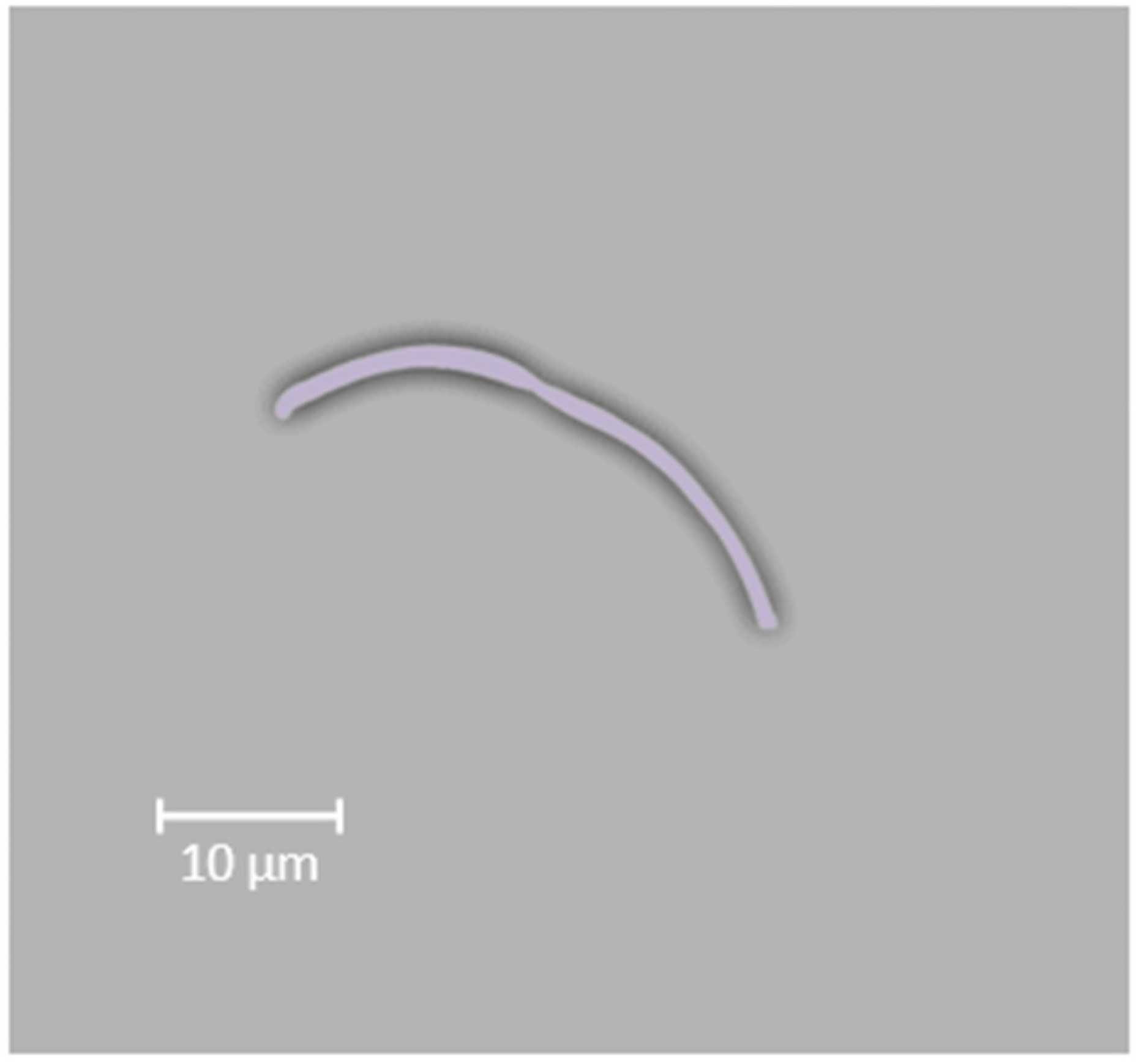
Due to the diversity of its origin, wide range of sizes, i.e., from 1 μm to 5 mm (in the case of large micro plastics), path of movement, density (low density favors transport, especially by wind [154]), chemical composition (different types of polymers), physical properties, such as various degrees of an effective surface affecting the formation of biofilms and absorbed pollutants, variety of shapes (balls, irregular particles, fibers, foils and foams), surface charge and hydrophobicity and many other features and properties, microplastics in the aquatic environment may be subject to high variability in terms of their occurrence and the changes and processes they undergoes. At the end of the last century, research on plastic particles mainly concerned the seas and oceans. The sizes of the tested particles mainly fell within the wide range for plastic garbage and particles of 1–2 mm in size were also marked and analyzed within them.
One of the disadvantages is the lack of a narrow definition of microplastic itself, as well as its size. The size ranges for microplastics found in the literature range from 50 mm to hundredths or even thousandths of a millimeter. For the needs of EU monitoring, a division into fractions of 1–5 mm and 20 µm–1 mm was recently proposed [155]. This chapter covers microplastics in the particle size range from 1 µm to 1000 µm [156] (Figure 3) and does not include nanoplastic due to how different its separation and identification methods are.
6.2. Collection, Extraction and Identification
A feature that makes it difficult to identify microplastic particles is that they are often mixtures of polymers, sometimes enriched with additives introduced during production. These properties must be taken into account when choosing an extraction method. MP extraction is the first stage and largely determines subsequent stages (in terms of the separation efficiency and unchanged form).
6.3. Sampling
In the case of inland waters, ten samples are taken from the water surface or water column. In addition to the water column and its surface, samples are also taken from sediments, e.g., using core samplers [157], and from beaches (one of the main problems is the dynamic changes of MP and beaches as well [150])—as a measure of microplastics floating on the surface (PP, PE) and carried by wind and waves on shore (methodology not covered by this chapter). In the simplest terms, the sampling methodology can be divided into three ways: total sampling (the entire volume is preserved, without reducing it during the sampling process)—it gives practically 100% certainty of the sampling effectiveness in terms of the mass of the collected material; however, such material may be strongly mixed with other particles, including organic ones, and will require further separation procedures, often labor-intensive, selective (direct sampling of fractions that are recognizable to the naked eye as plastic) and with a reduced volume—and thickening sampling using a net where various types of clogging of the pores (mesh) of the nets by the material collected may also occur [150].
In microplastics’ monitoring, it is problematic to have a large area, volume and depth of natural water reservoirs in the aquatic environment. This often determines the need to collect samples, leading to their compaction using various kinds of nets or meshes. These methods are relatively effective in the context of compaction. However, their disadvantage is the possibility of the omission a specific type of material, among other things, as a result of the misapplication of a certain size of mesh (net). The most commonly used nets are [158] Manta net [159,160] with a lower limit: 300 µm, Neuston net (lower limit: 333 µm), plankton net (lower limit: 100 µm), autosampler and microplastic catcher (100–333 µm). Waves caused by both wind and drone or ship movements can be a problem when collecting samples, causing disturbances in the accuracy of sampling in plan and vertically.
Microplastic particles can have different sizes and shapes. Some of the particles with specific shapes are fibrous or significantly elongated particles. The collection of fibrous particles using a net may be accompanied by a large error—the effectiveness of stopping a particle with a large disproportion in length to diameter depends on its position when it comes into contact with the mesh. Particles that do not come from the sample being tested may cause significant errors in the results of field tests. These include: particles from the air, researchers’ clothing and the material (paint) used to cover a ship, drone or boat. This material may also come from research equipment. An interesting and alternative solution in sampling is fraction filtering—water pressure even above 1 m3 through a filter cascade [161]. A promising technique is using the fluorescence of particles, e.g., eaten by vertebrates and invertebrates (using fluorescence and coherent anti-Stokes Raman scattering—CARS) [7].
6.4. Extraction—Density Separation, Filtration and Etching
One of the most commonly used methods of extracting microplastics due to their known and relatively constant density is density separation [156]. The density of plastic affects its distribution in the water profile. A material with a density smaller than water will tend to float or remain near the water surface. A material with a density similar to water will be moved in the water body profile, depending on the water currents, moving up and down, often to a large extent. A material with a density greater than water, e.g., PET and PVC, will tend to sediment and often accumulate in bottom sediments. Solutions for polymer density separation are chosen according to material properties (density) and its extraction efficiency depends on the shape and dimensions of MPs. One of the most popular for PE and PP is NaCl [162,163], zinc chloride solutions are used for materials of 1.5–1.7 g/cm3 [164,165] and sodium polytungstate is used for materials with a density of 1.4 g/cm3 [166].
The techniques used for extraction include a Microplastic Sediment Separator (MPSS) technique and elutriation with subsequent flotation [164].
Optionally, sieving through a 500 μm sieve is used if the solution contains fractions with larger particle sizes [167,168]. Vacuum filtration (sieving and suction) is also used for re-filtration [156]—Buchner filters are often used. The pore size of the filters can be in quite a wide range: from 1–2 μm (Al2O2) to 5 μm (silver, silicone) [156].
Further analytical procedures (visual-light or chemical) require pure samples. To remove the remains of biological (organic) substances, in addition to the manual elimination of relatively large particles (pieces of wood, large fragments of biofilm), treatment with an appropriate substance is used that will dissolve small or adhering plastic particles (soft tissues of flora and fauna) and which may make their identification difficult. Rinsing with fresh water is one of the most frequently used and safest components for MP structure and composition. The ultrasonic cleaning of aged and brittle MP may lead to its cracking [166]. For etching, the following are also used, among others: H2O2—e.g., 30% solution [165], HCL, NaOH, Fe(II) and H2O2, KOH [161], enzymes—e.g., proteinase-K [167] or, before FTIR, lipase, amylase, proteinase, chitinase, cellulase [162] and corolase, in combination with KOH [162]. Mineral acids are mainly used to decompose organic pollutants. The mixtures of acids, alkali and oxidants (hydrogen peroxide) or hot NO3 can also be used for the digestion of biotic tissues.
Some polymers, e.g., polyamide, polyoxymethylene and polycarbonate, cannot be cleaned with strong acids or alkali due to their reaction with them [165].
6.5. Visual Sorting, Visual Identification and Chemical Identification
Visual sorting should only be used for particles over 500 μm or even 1000 μm. If more accurate methods are not used (e.g., FTIR, Raman spectroscopy) [150], the visual sorting error level ranges from 20% [169] to 70% and increases with the decreasing particle size. Sorting chambers (e.g., a Bogorov counting chamber) can be used to sort water samples [150] and a dissecting microscope can be used to sort smaller particles [170].
Visual identification methods used to characterize MP include microscopic, spectroscopic and chromatographic techniques [171,172]. The following PMs’ boundary dimensions can be distinguished as AFM-IR—100 nm; SEM—0.1 µm–1.0 µm; R-spectroscopy—1.0 µm; FTIR/µFTIR > 10 µm; LM (light microscopy)—100 µm; and ATR-FTIR > 500 µm [173]. The procedure for the identification and characterization of MP in addition to the analysis of the size (boundary conditions determined at the sampling stage), shape, color and polymer identification.
Currently, various techniques are used to identify microplastics [174]. Spectroscopic and chemical techniques have recorded significant progress in the last dozen years. The wide spectrum of techniques for identifying polymer microparticles includes optical microscopy [175]; physico-chemical methods, including SEM [169,176]; spectroscopic techniques such as Fourier-transform infrared spectroscopy, FTIR [177,178], ATR-FTIR and Raman spectrometry [177]; thermal methods [179] (TGA, DSC); and chromatographic techniques (GC, HPLC).
Some of them are included in the SOP: µ-FTIR, ATR-FTIR, µ-Raman and Py-GC/MS. The SOP recommends using µ-FTIR and ATR-FTIR to clearly determine the polymer type. The use of the µ-Raman and Py-GC-MS techniques results in the destruction of the sample due to using too high a level of excitation energy [154], and the results are in the form of the mass (not the number of particles) in the case of Py-GC/MS and time consumption in the case of µ-Raman [159].
In the case of FTIR, the generated spectroscopic spectrum reflects the molecular structure of the sample, and the Fourier transformation is used to convert the signals. The principle of the operation of Fourier transform infrared spectroscopy (FTIR) is based on the interaction of infrared radiation with plastic particles, thanks to which a spectrum is obtained with characteristic bands corresponding to the specific vibrations of chemical groups [148]. Spectroscopy techniques involve the comparison of absorption and emission spectra with reference spectra [150]. This method is characterized by simplicity, effectiveness, non-invasiveness and reliability [179]. In recent years, automated FTIR techniques have also been used as they enable the fast analysis of thousands of spectra [179]. FTIR uses two measurement modes: reflectance and transmittance. Both have certain limitations—the first is that the irregular shape of the MP can result in spectra that are difficult to interpret, and the second is that it requires IR-transparent filters (e.g., alumina) and has limitations regarding sample thickness [122]. The drawbacks are, among others, that the lower size limit is 10–20 µm, there are difficulties in the case of a lack of sample transparency and water must be removed from the sample bore detection and organic fraction, e.g., biofilm disturbance detection [179].
Preparing a sample for the µ-FTIR method is relatively simple, but time-consuming [171]. It allows for the identification of particles between 10 and 20 µm in size. FTIR and µ-FTIR spectroscopies have been used in numerous studies of environmental samples [180]. The µ-FTIR is an FTIR system extended with a microscope which allows the analysis of particles below 500 µm. An additional advantage of FTIR is the ability to obtain information on aging (physical and chemical weathering) [166]. There is also a method of extending FTIR based on a focal array (FPA), thanks to which, by combining FPA fields, entire samples can be examined in detail as a total number of MPs, thanks to the simultaneous registration of several thousand spectra during one measurement [161].
One of the limitations of IR spectroscopy is the need to dry the sample before measurement due to the absorption of IR radiation by water; for the same reason, the determination of black particles may also cause problems. ATR-FTIR is used to analyze larger (due to the technical limitations of pressing small particles in a pressure camera) polymer particles as it is reflectance-mode FTIR spectroscopy [154]. It is a surface technique (IR radiation penetrates to a depth of 0.5 to 5.0 µm). This technique allows one to analyze MP with high precision and in a short time (less than 1 min).
Another technique, used with high reliability [7,156,164,180], is Raman Spectroscopy (RS). Its principle of operation is the interaction of photons emitted by the monochromatic laser light (wave length 500 to 800 nm) with plastic molecules in the form of, for example, vibrations and rotation [181]. This technique allows for the identification of a wide range of particle sizes, even below 1 µm. Thanks to the combination with CLSM, it allows the localization of MPs in biological tissues [7]. The generation of heat associated with excessive light absorption by the sample leads to its thermal degradation [182]. Raman spectroscopy has several advantages over FTIR, including non-contact measurements, the detecting of small particles with a diameter of 1 to 20 µm at high spatial resolution, automatic and fast data collection and processing [179] and the ability to analyze wet samples [183]. It has some disadvantages also, e.g., samples containing organic material residuals can disturb the generation of the Raman spectra that could be interpreted. This problem can be solved by using a longer wave length—longer than 1000 nm [161]. During the Raman technique, samples must be cleaned for proper MP identification. Microscopy coupled with a Raman spectrometer, called µ-Raman spectroscopy, allows for the identification of particles (thanks to comparing the generated spectra with a database containing reference spectra) with a diameter below 20 µm and to about 1 µm [182]. The advantage of using coupled FTIR with Raman spectroscopy is that they complement each other to some extent—molecular vibrations that are inactive in the Raman technique are active in infrared [161].
A relatively novel group of techniques are thermal analyses (e.g., thermal extraction and desorption using GC/MS, GC/MS, DSC). A promising technique is Py-GC/MS, which can provide information not only about the polymer, but also about the additives used [184]. The conventional Pyr-GC/MS needs to place MP particles manually in the pyrolitic tube. The principle of the operation of Pyr-GC/MS is the analysis of products formed as a result of the thermal degradation of the sample by pyrolysis [181,185]. The resulting gas mixture is separated into individual chemical compounds in a chromatographic column and generated spectra should be compared with a reference database [182]. The NMR, quantitative 1 H-NMR spectroscopy using bench top NMR and NoD methods, are also used for MP identification [186,187]. Thermal techniques such as TGA and DCS are utilized too [174], as well as chromatographic techniques, such as GC and HPLC [174]. More complex samples can be analyzed by combining mass spectrometry with thermogravimetric analysis and thermal desorption gas chromatography (TD-GC/MS).
Thermal methods, apart from several significant advantages, such as a large sample volume (TD-GC/MS) and the ability to detect various types of polymers, also have some disadvantages, including sample destruction, the process length (Pyr-GC/MS) and the influence of substrate purity (DSC) [179]. GC/MS pyrolysis can also be combined with pressurized liquid extraction (PLE) or automatic pressure liquid extraction (APLE) to achieve low detection limits. During this procedure, however, care must be taken when grinding and homogenizing the samples due to the formation of agglomerates [188].
Often, in order to obtain results with lower uncertainty (error) or a greater range of information (such as applicability to small-sized particles), combinations of methods are used [189], e.g., pyrolysis with gas chromatography and mass spectrometry (Pyr-GC/MS), FTIR/optical microscopy (µ-FTIR), thermogravimetry with differential scanning calorimetry (TGA-DSC), gas chromatography with thermal desorption and mass spectrometry (TED-GC/MS) and RS/microscopy (µ-Raman) [171].
The thermal analytical method combining TGA-SPE and TDS-GC/MS is thermal extraction–desorption–gas chromatography–mass spectrometry (TED-GC/MS) [190]. A high temperature is used—nearly 1000 °C. The advantage of this method is shortening the analysis time of large samples with a relatively large sample weight (up to 100 mg). Thanks to differential scanning calorimetry (DSC) [179], substances can be identified qualitatively and quantitatively by measuring the melting point of an MP sample heated to different temperatures [191]. The method is simple and relatively cheap. Due to the novelty of this method, reference materials are not yet available. In the case of large particles, a difficulty may be their higher mass-to-surface ratio [192].
Another promising technique is Cloud-point extraction (CPE) [193]. MP is isolated from liquid samples using non-ionized surfactants (e.g., Triton X-45), which, when heated to a certain temperature, form clouds (the so-called cloud point when the surfactant concentration exceeds the critical micelle concentration—CMC), thus separating from the bulk solution [193].
6.6. Counting and Data Presenting
The last stage is usually counting, organizing the obtained results and presenting them using commonly used and representative units, including the number of particles per unit of mass, the number of particles per unit of volume, the mass of particles per unit of mass and the mass of particles per unit of volume. Optionally, a unit of mass or number of particles per unit area of the body of water is used. To summarize the discussion so far, although identification micro-FTIR and micro-Raman techniques are still very popular and used successfully for much smaller particle sizes in individual cases, it is recommended to use 100 μm as the lower particle size limit due to the limitations of the currently used techniques [154]. The main problems relating to MPs’ identification are the lack of unification, standardization and repeatability of the methods used in these studies [154]. The discrepancies concern both the use of different methods (including analytical ones), as well as technical details within the same methods (concentrations of reagents, digestion time and process temperature). When sampling microplastics in the future, such factors and conditions should be taken into account: the precise control of a boat or drone and cruise planning—both in terms of the precision of sampling in the top view and in the vertical cross-section of the reservoir. It is best for the cruise plan to be automated, with simultaneous corrections due to water waves, wind and possible currents in the water column.
The efficiency of extraction using classic methods for small particles (40–300 µm) is still relatively low—on average 40% [164]. Newer methods show a higher efficiency of up to 100%. The high extraction rate of the recovery of small microplastics gives an MPSS of 96% [164]. Procedures and strategies (SOP, BASEMEN, SCS and others) should also be maintained [160]. With the computational opportunities of IT systems growing at a significant pace, it seems possible to combine the identification elements resulting from the SOP and SCS systems, i.e., combining quantitative parameters (mass and number of particles) with qualitative parameters (particle size, color, shape, etc.). Modern methods, such as the use of AI, methods based on remote sensing and other interesting methods, such as the analysis of data from extensive Internet or other data sources [194] and the consumption of microplastics by vertebrates, should be improved regardless of the development of the most popular methods. The methodology of MPs’ identification requires refinement at every stage—arranging size categories, sampling and extraction—and the method of interpreting and reporting quantitative and qualitative results [156] and robust standards and procedures (e.g., QAQC) should be developed, as in other areas of analytical chemistry.
There are still discrepancies in the consideration of MP properties; one of the reasons is the lack of the sufficient harmonization of sample collection and analysis methods [22]. In the near future, in order to improve the identification and elimination of MPs, the use of electrochemical methods will probably be widespread due to their low cost, high sensitivity and easiness to use; however, in the case of large MPs or aggregates, problems may occur. Therefore, it seems advisable to develop multi-channel sensors—electrodes [179]. In the coming years, it can be expected that innovative techniques will be used in both micro- and nano-plastic detection, such as confocal laser scanning microscopy, laser particle size analysis, flow cytometry or dynamic light scattering analysis. This will be facilitated by the integration of various research fields (e.g., materials science and environmental medicine) [195].
7. Conclusions
In time, when, together with a water shortage, other problems have been present for years or are just emerging, it seems that it will be necessary to develop new concepts and more precise methods of studies. The observed water scarcity coupled with water eutrophication, intensive agriculture, the presence of xenobiotics and microplastics in waters, the destruction of natural biota, the presence of various industrial effluents including mine waters, the decline of biodiversity and many places with biological invasions are becoming increasingly prevalent issues, thus the need to prevent them, based on the properly collected data, is apparent.
Recent studies, which include methods using UAVs and UAS, which have a low impact on the aquatic environment, can assure undisturbed physico-chemical, toxicological and biological samples. They can enable results to be obtained from areas normally beyond the reach of researchers, such as the rapidly changing Arctic regions. New methods and paradigms could not only help to collect samples or key environmental data using remote systems, but can also be very useful for biodiversity conservation works due to their still-developing capabilities. They can be used in assessing the direction of changes in water quality, including determining the length of the zone of complete mixing, and in biological assessments, like the presence of chlorophyll in the waters.
An aspect that is currently of great concern to researchers is the widespread presence of microplastics in freshwater. Today, there are some inconsistencies in the describing of different properties of microplastics. Thus, the aforementioned lack of coordination of sampling procedures and incoherent analytic methods should be urgently solved. In order to improve the identification and elimination of microplastics from inland waters, new low-cost methods need to be implemented in this decade.
In this paper, the authors have outlined only some of the main threats and challenges facing modern science, but even these few pressing environmental issues show how much can and should be done to save inland waters.
Author Contributions
R.S., B.M., P.D., P.B. and M.S. contributed equally to manuscript preparation. All authors have read and agreed to the published version of the manuscript.
Funding
This research was partially funded by Polish Ministry of Science and Higher Education, grant number 506.868.06.00/UP.
Data Availability Statement
The data presented in this study are available on request from the corresponding author.
Conflicts of Interest
The authors declare no conflicts of interest.
Abbreviations
| AMD | acid mine drainage |
| AOTF | acousto-optic tunable filter |
| AFM | atomic force microscopy |
| APLE | automatic pressure liquid extraction |
| ATR | attenuated total reflectance |
| BASEMAN | baselines and standards for microplastics analyses |
| CARS | fluorescence and coherent anti-Stokes Raman scattering |
| ChlF | chlorophyll a fluorescence |
| CLSM | confocal laser scanning microscopy |
| CMC | critical micelle concentration |
| CMP | complete mixing path |
| CPE | cloud-point extraction |
| DO | dissolved oxygen |
| DSC | differential scanning calorimetry |
| EDS | energy dispersive X-ray spectroscopy |
| FPA | focal plane array |
| FTIR | Fourier-transform infrared spectroscopy |
| GC | gas chromatography |
| HAB | harmful algal bloom |
| H-NMR | proton nuclear magnetic resonance |
| HPLC | high-performance liquid chromatography |
| NAP | non-algal particles |
| NMR | nuclear magnetic resonance |
| MP | microplastic |
| MPSS | microplastic–sediment separator |
| MW | mine waters |
| PAR | photosynthetically active radiation |
| PE | polyethylene |
| PET | polyethylene terephthalate |
| PP | polypropylene |
| PVC | polyvinyl chloride |
| Pyr-GC/MS | pyrolysis–gas chromatography–mass spectrometry |
| QAQC | quality assurance and quality control |
| RS | Raman Spectroscopy |
| SCS | Swiss Chemical Society |
| SEM | scanning electron microscope |
| SIF | Sun-Induced Chlorophyll Fluoresence |
| SOP | Standard Operating Procedure |
| SPE | Solid-phase extraction |
| TDS-GC/MS | thermodesorption gas chromatography with mass spectrometric detection |
| TED-GC/MS | automated thermal extraction—desorption gas chromatography mass spectrometry |
| TGA | thermal gravimetric analysis |
| UAV | unmanned aerial vehicle |
| UAS | unmanned aerial system |
References
- Behrenfeld, M.J.; Westberry, T.K.; Boss, E.S.; O’Malley, R.T.; Siegel, D.A.; Wiggert, J.D.; Franz, B.A.; McClain, C.R.; Feldman, G.C.; Doney, S.C.; et al. Satellite-Detected Fluorescence Reveals Global Physiology of Ocean Phytoplankton. Biogeosciences 2009, 6, 779–794. [Google Scholar] [CrossRef]
- Marszelewski, W.; Dembowska, E.A.; Napiórkowski, P.; Solarczyk, A. Understanding abiotic and biotic conditions in post-mining pit lakes for efficient management: A case study (Poland). Mine Water Environ. 2017, 36, 418–428. [Google Scholar] [CrossRef]
- Malea, L.; Nakou, K.; Papadimitriou, A.; Exadactylos, A.; Orfanidis, S. Physiological Responses of the Submerged Macrophyte Stuckenia pectinata to High Salinity and Irradiance Stress to Assess Eutrophication Management and Climatic Effects: An Integrative Approach. Water 2021, 13, 1706. [Google Scholar] [CrossRef]
- Ji, S.; Ma, S. The effects of industrial pollution on ecosystem service value: A case study in a heavy industrial area, China. Environ. Dev. Sustain. 2022, 24, 6804–6833. [Google Scholar] [CrossRef]
- Cheng, L.; Tan, X.; Yao, D.; Xu, W.; Wu, H.; Chen, Y. A Fishery Water Quality Monitoring and Prediction Evaluation System for Floating UAV Based on Time Series. Sensors 2021, 21, 4451. [Google Scholar] [CrossRef] [PubMed]
- Messyasz, B.; Pikosz, M.; Treska, E. Biology of freshwater macroalgae and their distribution. In Algae Biomass: Characteristics and Applications; Springer: Berlin/Heidelberg, Germany, 2018; Volume 8, pp. 17–31. [Google Scholar] [CrossRef]
- Cole, M.; Lindeque, P.; Fileman, E.; Halsband, C.; Goodhead, R.; Moger, J.; Galloway, T.S. Microplastic ingestion by zooplankton. Environ. Sci. Technol. 2013, 47, 6646–6655. [Google Scholar] [CrossRef] [PubMed]
- Staniszewski, R.; Niedzielski, P.; Sobczyński, T.; Sojka, M. Trace Elements in Sediments of Rivers Affected by Brown Coal Mining: A Potential Environmental Hazard. Energies 2022, 15, 2828. [Google Scholar] [CrossRef]
- Cheng, K.H.; Jiao, J.J.; Luo, X.; Yu, S. Effective Coastal Escherichia Coli Monitoring by Unmanned Aerial Vehicles (UAV) Thermal Infrared Images. Water Res. 2022, 222, 118900. [Google Scholar] [CrossRef] [PubMed]
- Duysens, L.N.M.; Sweers, H.E. Mechanisms of two photochemical reactions in algae as studied by means of fluorescence. In Studies on Microalgae and Photosynthetic Bacteria, Special Issue of Plant Cell Physiol; Mahlis, L., Ed.; Japanese Society of Plant Physiologists; University of Tokyo Press: Tokyo, Japan, 1963; pp. 353–372. [Google Scholar]
- Turnau, K.; Płachno, B.J.; Bień, P.; Świątek, P.; Dąbrowski, P.; Kalaji, H. Fungal symbionts impact cyanobacterial biofilm durability and photosynthetic efficiency. Curr. Biol. 2023, 33, 5257–5262.e3. [Google Scholar] [CrossRef] [PubMed]
- Hancock, S.; Wolkersdorfer, C. Renewed demands for mine water management. Mine Water Environ. 2012, 31, 147–158. [Google Scholar] [CrossRef]
- Staniszewski, R.; Diatta, J.B.; Andrzejewska, B. Impact of lignite mine waters from deep seated drainage on water quality of the Noteć River. J. Elem. 2014, 19, 749–758. [Google Scholar] [CrossRef]
- Akanle, O.; Adejare, G.S.; Adewusi, A.O.; Yusuf, Q.O. Farmers-Herders Conflicts and Development in Nigeria. Niger. J. Sociol. Anthropol. 2021, 19, 1. [Google Scholar] [CrossRef]
- Talozi, S.; Altz-Stamm, A.; Hussein, H.; Reich, P. What constitutes an equitable water share? A reassessment of equitable apportionment in the Jordan–Israel water agreement 25 years later. Water Policy 2019, 21, 911–933. [Google Scholar] [CrossRef]
- Wheeler, K.G.; Hall, J.W.; Abdo, G.M.; Dadson, S.J.; Kasprzyk, J.R.; Smith, R.; Zagona, E.A. Exploring cooperative transboundary river management strategies for the Eastern Nile Basin. Water Resour. Res. 2018, 54, 9224–9254. [Google Scholar] [CrossRef] [PubMed]
- Wheeler, K.G.; Hussein, H. Water research and nationalism in the post-truth era. Water Int. 2021, 46, 1216–1223. [Google Scholar] [CrossRef]
- Shelare, S.D.; Aglawe, K.R.; Waghmare, S.N.; Belkhode, P.N. Advances in Water Sample Collections with a Drone—A Review. Mater. Today Proc. 2021, 47, 4490–4494. [Google Scholar] [CrossRef]
- Guareschi, S.; Laini, A.; England, J.; Barrett, J.; Wood, P.J. Multiple co-occurrent alien invaders constrain aquatic biodiversity in rivers. Ecol. Appl. 2021, 31, e02385. [Google Scholar] [CrossRef]
- Dubelaar, G.B.; Geerders, P.J.; Jonker, R.R. High frequency monitoring reveals phytoplankton dynamics. J. Environ. Monit. 2004, 6, 946–952. [Google Scholar] [CrossRef]
- Srivastav, S.K.; Yadav, H.L.; Seervi, V.; Jamal, A. Assessment of water quality near vicinity of lignite mine region, Gujarat, India: A case study. Int. Adv. Res. J. Sci. Eng. Technol. 2017, 4, 42–47. [Google Scholar]
- Hartmann, N.B.; Huffer, T.; Thompson, R.C.; Hassellöv, M.; Verschoor, A.; Daugaard, A.E.; Rist, S.; Karlsson, T.; Brennholt, N.; Cole, M.; et al. Are we speaking the same language? Recommendations for a definition and categorization framework for plastic debris. Environ. Sci. Technol. 2019, 53, 1039–1047. [Google Scholar] [CrossRef]
- Guimarães, T.T.; Veronez, M.R.; Koste, E.C.; Souza, E.M.; Brum, D.; Gonzaga, L.; Mauad, F.F. Evaluation of Regression Analysis and Neural Networks to Predict Total Suspended Solids in Water Bodies from Unmanned Aerial Vehicle Images. Sustainability 2019, 11, 2580. [Google Scholar] [CrossRef]
- Wei, L.; Huang, C.; Zhong, Y.; Wang, Z.; Hu, X.; Lin, L. Inland Waters Suspended Solids Concentration Retrieval Based on PSO-LSSVM for UAV-Borne Hyperspectral Remote Sensing Imagery. Remote Sens. 2019, 11, 1455. [Google Scholar] [CrossRef]
- Chicuazuque, C.; Sarmiento, J.; Rodríguez, J.; Upegui, E. Total Suspended Solids (TSS) Estimation Over a Section of the Upper Bogota River Basin (Colombia) through Processing Multispectral Images Captured Using UAV. In Proceedings of the 2021 IEEE International Geoscience and Remote Sensing Symposium IGARSS, Brussels, Belgium, 11–16 July 2021; pp. 8189–8192. [Google Scholar]
- Prior, E.M.; O’Donnell, F.C.; Brodbeck, C.; Donald, W.N.; Runion, G.B.; Shepherd, S.L. Measuring High Levels of Total Suspended Solids and Turbidity Using Small Unoccupied Aerial Systems (SUAS) Multispectral Imagery. Drones 2020, 4, 54. [Google Scholar] [CrossRef]
- Hou, Y.; Zhang, A.; Lv, R.; Zhang, Y.; Ma, J.; Li, T. Machine learning algorithm inversion experiment and pollution analysis of water quality parameters in urban small and medium-sized rivers based on UAV multispectral data. Environ. Sci. Pollut. Res. 2023, 30, 78913–78932. [Google Scholar] [CrossRef] [PubMed]
- Cui, M.; Sun, Y.; Huang, C.; Li, M. Water Turbidity Retrieval Based on UAV Hyperspectral Remote Sensing. Water 2022, 14, 128. [Google Scholar] [CrossRef]
- Bussières, S.; Kinnard, C.; Clermont, M.; Campeau, S.; Dubé-Richard, D.; Bordeleau, P.-A.; Roy, A. Monitoring Water Turbidity in a Temperate Floodplain Using UAV: Potential and Challenges. Can. J. Remote Sens. 2022, 48, 565–574. [Google Scholar] [CrossRef]
- McEliece, R.; Hinz, S.; Guarini, J.-M.; Coston-Guarini, J. Evaluation of Nearshore and Offshore Water Quality Assessment Using UAV Multispectral Imagery. Remote Sens. 2020, 12, 2258. [Google Scholar] [CrossRef]
- Zhang, L.; Han, W.; Niu, Y.; Chávez, J.L.; Shao, G.; Zhang, H. Evaluating the Sensitivity of Water Stressed Maize Chlorophyll and Structure Based on UAV Derived Vegetation Indices. Comput. Electron. Agric. 2021, 185, 106174. [Google Scholar] [CrossRef]
- Gai, Y.; Yu, D.; Zhou, Y.; Yang, L.; Chen, C.; Chen, J. An Improved Model for Chlorophyll-a Concentration Retrieval in Coastal Waters Based on UAV-Borne Hyperspectral Imagery: A Case Study in Qingdao, China. Water 2020, 12, 2769. [Google Scholar] [CrossRef]
- Kim, E.-J.; Nam, S.-H.; Koo, J.-W.; Hwang, T.-M. Hybrid Approach of Unmanned Aerial Vehicle and Unmanned Surface Vehicle for Assessment of Chlorophyll-a Imagery Using Spectral Indices in Stream, South Korea. Water 2021, 13, 1930. [Google Scholar] [CrossRef]
- Guimarães, T.T.; Veronez, M.R.; Koste, E.C.; Gonzaga, L.; Bordin, F.; Inocencio, L.C.; Larocca, A.P.C.; De Oliveira, M.Z.; Vitti, D.C.; Mauad, F.F. An Alternative Method of Spatial Autocorrelation for Chlorophyll Detection in Water Bodies Using Remote Sensing. Sustainability 2017, 9, 416. [Google Scholar] [CrossRef]
- Zhao, X.; Li, Y.; Chen, Y.; Qiao, X.; Qian, W. Water Chlorophyll a Estimation Using UAV-Based Multispectral Data and Machine Learning. Drones 2023, 7, 2. [Google Scholar] [CrossRef]
- Pyo, J.C.; Ligaray, M.; Kwon, Y.S.; Ahn, M.-H.; Kim, K.; Lee, H.; Kang, T.; Cho, S.B.; Park, Y.; Cho, K.H. High-Spatial Resolution Monitoring of Phycocyanin and Chlorophyll-a Using Airborne Hyperspectral Imagery. Remote Sens. 2018, 10, 1180. [Google Scholar] [CrossRef]
- Logan, R.D.; Torrey, M.A.; Feijó-Lima, R.; Colman, B.P.; Valett, H.M.; Shaw, J.A. UAV-Based Hyperspectral Imaging for River Algae Pigment Estimation. Remote Sens. 2023, 15, 3148. [Google Scholar] [CrossRef]
- Kwon, Y.S.; Pyo, J.; Kwon, Y.-H.; Duan, H.; Cho, K.H.; Park, Y. Drone-Based Hyperspectral Remote Sensing of Cyanobacteria Using Vertical Cumulative Pigment Concentration in a Deep Reservoir. Remote Sens. Environ. 2020, 236, 111517. [Google Scholar] [CrossRef]
- Pyo, J.; Hong, S.M.; Jang, J.; Park, S.; Park, J.; Noh, J.H.; Cho, K.H. Drone-Borne Sensing of Major and Accessory Pigments in Algae Using Deep Learning Modeling. GIsci. Remote Sens. 2022, 59, 310–332. [Google Scholar] [CrossRef]
- Fernandez-Figueroa, E.G.; Wilson, A.E.; Rogers, S.R. Commercially Available Unoccupied Aerial Systems for Monitoring Harmful Algal Blooms: A Comparative Study. Limnol. Oceanogr. Methods 2022, 20, 146–158. [Google Scholar] [CrossRef]
- Yan, Y.; Wang, Y.; Yu, C.; Zhang, Z. Multispectral Remote Sensing for Estimating Water Quality Parameters: A Comparative Study of Inversion Methods Using Unmanned Aerial Vehicles (UAVs). Sustainability 2023, 15, 298. [Google Scholar] [CrossRef]
- Bartz, R.L.; Feiden, A. Water Transparency Analysis in Fish Farming Environment through Unmanned Aerial Vehicles. J. Appl. Res. Technol. 2023, 21, 912–920. [Google Scholar] [CrossRef]
- Wei, L.; Wang, Z.; Huang, C.; Zhang, Y.; Wang, Z.; Xia, H.; Cao, L. Transparency Estimation of Narrow Rivers by UAV-Borne Hyperspectral Remote Sensing Imagery. IEEE Access 2020, 8, 168137–168153. [Google Scholar] [CrossRef]
- Qun’ou, J.; Lidan, X.; Siyang, S.; Meilin, W.; Huijie, X. Retrieval Model for Total Nitrogen Concentration Based on UAV Hyper Spectral Remote Sensing Data and Machine Learning Algorithms—A Case Study in the Miyun Reservoir, China. Ecol. Indic. 2021, 124, 107356. [Google Scholar] [CrossRef]
- Wang, J.; Shi, T.; Yu, D.; Teng, D.; Ge, X.; Zhang, Z.; Yang, X.; Wang, H.; Wu, G. Ensemble Machine-Learning-Based Framework for Estimating Total Nitrogen Concentration in Water Using Drone-Borne Hyperspectral Imagery of Emergent Plants: A Case Study in an Arid Oasis, NW China. Environ. Pollut. 2020, 266, 115412. [Google Scholar] [CrossRef] [PubMed]
- Seoung-Hyeon, K.; Byung-Hyun, M.; Bong-Geun, S.; Kyung-Hun, P. An Analysis on the Usability of Unmanned Aerial Vehicle(UAV) Image to Identify Water Quality Characteristics in Agricultural Streams. J. Korean Assoc. Geogr. Inf. Stud. 2019, 22, 10–20. [Google Scholar] [CrossRef]
- Liu, J.; Ding, J.; Ge, X.; Wang, J. Evaluation of Total Nitrogen in Water via Airborne Hyperspectral Data: Potential of Fractional Order Discretization Algorithm and Discrete Wavelet Transform Analysis. Remote Sens. 2021, 13, 4643. [Google Scholar] [CrossRef]
- Koparan, C.; Koc, A.B.; Privette, C.V.; Sawyer, C.B. Autonomous In Situ Measurements of Noncontaminant Water Quality Indicators and Sample Collection with a UAV. Water 2019, 11, 604. [Google Scholar] [CrossRef]
- Sandu, M.A.; Vîrsta, A.; Scăețeanu, G.V.; Iliescu, A.-I.; Ivan, I.; Nicolae, C.G.; Stoian, M.; Madjar, R.M. Water Quality Monitoring Of Moara Domnească Pond, Ilfov County, Using Uav-Based Rgb Imaging. Agrolife Sci. J. 2023, 12, 191–201. [Google Scholar] [CrossRef]
- Hu, W.; Liu, J.; Wang, H.; Miao, D.; Shao, D.; Gu, W. Retrieval of TP Concentration from UAV Multispectral Images Using IOA-ML Models in Small Inland Waterbodies. Remote Sens. 2023, 15, 1250. [Google Scholar] [CrossRef]
- Chen, B.; Mu, X.; Chen, P.; Wang, B.; Choi, J.; Park, H.; Xu, S.; Wu, Y.; Yang, H. Machine Learning-Based Inversion of Water Quality Parameters in Typical Reach of the Urban River by UAV Multispectral Data. Ecol. Indic. 2021, 133, 108434. [Google Scholar] [CrossRef]
- Arango, J.G.; Nairn, R.W. Prediction of Optical and Non-Optical Water Quality Parameters in Oligotrophic and Eutrophic Aquatic Systems Using a Small Unmanned Aerial System. Drones 2020, 4, 1. [Google Scholar] [CrossRef]
- Taddia, Y.; Russo, P.; Lovo, S.; Pellegrinelli, A. Multispectral UAV Monitoring of Submerged Seaweed in Shallow Water. Appl. Geomat. 2020, 12, 19–34. [Google Scholar] [CrossRef]
- Kislik, C.; Dronova, I.; Kelly, M. UAVs in Support of Algal Bloom Research: A Review of Current Applications and Future Opportunities. Drones 2018, 2, 35. [Google Scholar] [CrossRef]
- Becker, R.H.; Sayers, M.; Dehm, D.; Shuchman, R.; Quintero, K.; Bosse, K.; Sawtell, R. Unmanned Aerial System Based Spectroradiometer for Monitoring Harmful Algal Blooms: A New Paradigm in Water Quality Monitoring. J. Great Lakes Res. 2019, 45, 444–453. [Google Scholar] [CrossRef]
- Novković, M.; Cvijanović, D.; Minučer, M.; Pavić, D.; Drešković, N.; Milošević, Đ.; Anđelković, A.; Damnjanović, B.; Radulović, S. Towards UAV Assisted Monitoring of an Aquatic Vegetation within the Large Rivers—The Middle Danube. Carpathian J. Earth Environ. Sci. 2023, 18, 307–322. [Google Scholar] [CrossRef]
- Flynn, K.F.; Chapra, S.C. Remote Sensing of Submerged Aquatic Vegetation in a Shallow Non-Turbid River Using an Unmanned Aerial Vehicle. Remote Sens. 2014, 6, 12815–12836. [Google Scholar] [CrossRef]
- Chabot, D.; Dillon, C.; Shemrock, A.; Weissflog, N.; Sager, E.P.S. An Object-Based Image Analysis Workflow for Monitoring Shallow-Water Aquatic Vegetation in Multispectral Drone Imagery. ISPRS Int. J. Geoinf. 2018, 7, 294. [Google Scholar] [CrossRef]
- Song, B.; Park, K. Detection of Aquatic Plants Using Multispectral UAV Imagery and Vegetation Index. Remote Sens. 2020, 12, 387. [Google Scholar] [CrossRef]
- Husson, E.; Hagner, O.; Ecke, F. Unmanned Aircraft Systems Help to Map Aquatic Vegetation. Appl. Veg. Sci. 2014, 17, 567–577. [Google Scholar] [CrossRef]
- Zeng, Y.; Meng, X.; Zhang, Y.; Dai, W.; Fang, N.; Shi, Z. Estimation of the Volume of Sediment Deposited behind Check Dams Based on UAV Remote Sensing. J. Hydrol. 2022, 612, 128143. [Google Scholar] [CrossRef]
- Larson, M.D.; Simic Milas, A.; Vincent, R.K.; Evans, J.E. Multi-Depth Suspended Sediment Estimation Using High-Resolution Remote-Sensing UAV in Maumee River, Ohio. Int. J. Remote Sens. 2018, 39, 5472–5489. [Google Scholar] [CrossRef]
- Wei, L.; Huang, C.; Wang, Z.; Wang, Z.; Zhou, X.; Cao, L. Monitoring of Urban Black-Odor Water Based on Nemerow Index and Gradient Boosting Decision Tree Regression Using UAV-Borne Hyperspectral Imagery. Remote Sens. 2019, 11, 2402. [Google Scholar] [CrossRef]
- Wang, F.; Hu, H.; Luo, Y.; Lei, X.; Wu, D.; Jiang, J. Monitoring of Urban Black-Odor Water Using UAV Multispectral Data Based on Extreme Gradient Boosting. Water 2022, 14, 3354. [Google Scholar] [CrossRef]
- Sarigai; Yang, J.; Zhou, A.; Han, L.; Li, Y.; Xie, Y. Monitoring Urban Black-Odorous Water by Using Hyperspectral Data and Machine Learning. Environ. Pollut. 2021, 269, 116166. [Google Scholar] [CrossRef] [PubMed]
- Wu, D.; Jiang, J.; Wang, F.; Luo, Y.; Lei, X.; Lai, C.; Wu, X.; Xu, M. Retrieving Eutrophic Water in Highly Urbanized Area Coupling UAV Multispectral Data and Machine Learning Algorithms. Water 2023, 15, 354. [Google Scholar] [CrossRef]
- Liu, H.; Yu, T.; Hu, B.; Hou, X.; Zhang, Z.; Liu, X.; Liu, J.; Wang, X.; Zhong, J.; Tan, Z.; et al. UAV-Borne Hyperspectral Imaging Remote Sensing System Based on Acousto-Optic Tunable Filter for Water Quality Monitoring. Remote Sens. 2021, 13, 469. [Google Scholar] [CrossRef]
- Smith, B.; Beman, M.; Gravano, D.; Chen, Y. Development and Validation of a Microbe Detecting UAV Payload. In Proceedings of the 2015 Workshop on Research, Education and Development of Unmanned Aerial Systems (RED-UAS), Cancun, Mexico, 23–25 November 2015; pp. 258–264. [Google Scholar]
- Morgan, B.J.; Stocker, M.D.; Valdes-Abellan, J.; Kim, M.S.; Pachepsky, Y. Drone-Based Imaging to Assess the Microbial Water Quality in an Irrigation Pond: A Pilot Study. Sci. Total Environ. 2020, 716, 135757. [Google Scholar] [CrossRef] [PubMed]
- Benson, J.; Hanlon, R.; Seifried, T.M.; Baloh, P.; Powers, C.W.; Grothe, H.; Schmale, D.G. Microorganisms Collected from the Surface of Freshwater Lakes Using a Drone Water Sampling System (DOWSE). Water 2019, 11, 157. [Google Scholar] [CrossRef]
- Cillero Castro, C.; Domínguez Gómez, J.A.; Delgado Martín, J.; Hinojo Sánchez, B.A.; Cereijo Arango, J.L.; Cheda Tuya, F.A.; Díaz-Varela, R. An UAV and Satellite Multispectral Data Approach to Monitor Water Quality in Small Reservoirs. Remote Sens. 2020, 12, 1514. [Google Scholar] [CrossRef]
- Adão, T.; Hruška, J.; Pádua, L.; Bessa, J.; Peres, E.; Morais, R.; Sousa, J.J. Hyperspectral Imaging: A Review on UAV-Based Sensors, Data Processing and Applications for Agriculture and Forestry. Remote Sens. 2017, 9, 110. [Google Scholar] [CrossRef]
- Ying, H.; Xia, K.; Huang, X.; Feng, H.; Yang, Y.; Du, X.; Huang, L. Evaluation of Water Quality Based on UAV Images and the IMP-MPP Algorithm. Ecol. Inform. 2021, 61, 101239. [Google Scholar] [CrossRef]
- Lu, Q.; Si, W.; Wei, L.; Li, Z.; Xia, Z.; Ye, S.; Xia, Y. Retrieval of Water Quality from UAV-Borne Hyperspectral Imagery: A Comparative Study of Machine Learning Algorithms. Remote Sens. 2021, 13, 3928. [Google Scholar] [CrossRef]
- Burdziakowski, P.; Zima, P.; Wielgat, P.; Kalinowska, D. Tracking Fluorescent Dye Dispersion from an Unmanned Aerial Vehicle. Sensors 2021, 21, 3905. [Google Scholar] [CrossRef] [PubMed]
- Filippi, M.; Hanlon, R.; Rypina, I.I.; Hodges, B.A.; Peacock, T.; Schmale, D.G. Tracking a Surrogate Hazardous Agent (Rhodamine Dye) in a Coastal Ocean Environment Using In Situ Measurements and Concentration Estimates Derived from Drone Images. Remote Sens. 2021, 13, 4415. [Google Scholar] [CrossRef]
- Baek, D.; Seo, I.W.; Kim, J.S.; Nelson, J.M. UAV-Based Measurements of Spatio-Temporal Concentration Distributions of Fluorescent Tracers in Open Channel Flows. Adv. Water Resour. 2019, 127, 76–88. [Google Scholar] [CrossRef]
- Powers, C.; Hanlon, R.; Schmale, D.G. Tracking of a Fluorescent Dye in a Freshwater Lake with an Unmanned Surface Vehicle and an Unmanned Aircraft System. Remote Sens. 2018, 10, 81. [Google Scholar] [CrossRef]
- Sharma, C.; Isha, I.; Vashisht, V. Water Quality Estimation Using Computer Vision in UAV. In Proceedings of the 2021 11th International Conference on Cloud Computing, Data Science & Engineering (Confluence), Noida, India, 28–29 January 2021; IEEE: Piscataway, NJ, USA, 2021; pp. 448–453. [Google Scholar]
- Etikasari, B.; Husin; Kautsar, S.; Riskiawan, H.Y.; Setyohadi, D.P.S. Wireless Sensor Network Development in Unmanned Aerial Vehicle (UAV) for Water Quality Monitoring System. IOP Conf. Ser. Earth Environ. Sci. 2020, 411, 012061. [Google Scholar] [CrossRef]
- Koparan, C.; Koc, A.B.; Privette, C.V.; Sawyer, C.B. In Situ Water Quality Measurements Using an Unmanned Aerial Vehicle (UAV) System. Water 2018, 10, 264. [Google Scholar] [CrossRef]
- Koparan, C.; Koc, A.B.; Privette, C.V.; Sawyer, C.B.; Sharp, J.L. Evaluation of a UAV-assisted autonomous water sampling. Water 2018, 10, 655. [Google Scholar] [CrossRef]
- Koparan, C.; Koc, A.B. Unmanned Aerial Vehicle (UAV) Assisted Water Sampling. In Proceedings of the 2016 ASABE International Meeting, Orlando, FL, USA, 17–20 July 2016; American Society of Agricultural and Biological Engineers: St. Joseph, MI, USA, 2016. [Google Scholar]
- Koparan, C.; Koc, A.B.; Privette, C.V.; Sawyer, C.B. Adaptive Water Sampling Device for Aerial Robots. Drones 2020, 4, 5. [Google Scholar] [CrossRef]
- Ore, J.-P.; Elbaum, S.; Burgin, A.; Detweiler, C. Autonomous Aerial Water Sampling. J. Field Robot. 2015, 32, 1095–1113. [Google Scholar] [CrossRef]
- Schwarzbach, M.; Laiacker, M.; Mulero-Pázmány, M.; Kondak, K. Remote Water Sampling Using Flying Robots. In Proceedings of the 2014 International Conference on Unmanned Aircraft Systems (ICUAS), Orlando, FL, USA, 27–30 May 2014; pp. 72–76. [Google Scholar]
- Koparan, C.; Koc, A.B.; Sawyer, C.; Privette, C. Temperature Profiling of Waterbodies with a UAV-Integrated Sensor Subsystem. Drones 2020, 4, 35. [Google Scholar] [CrossRef]
- Doi, H.; Akamatsu, Y.; Watanabe, Y.; Goto, M.; Inui, R.; Katano, I.; Nagano, M.; Takahara, T.; Minamoto, T. Water Sampling for Environmental DNA Surveys by Using an Unmanned Aerial Vehicle. Limnol. Oceanogr. Methods 2017, 15, 939–944. [Google Scholar] [CrossRef]
- Terada, A.; Morita, Y.; Hashimoto, T.; Mori, T.; Ohba, T.; Yaguchi, M.; Kanda, W. Water Sampling Using a Drone at Yugama Crater Lake, Kusatsu-Shirane Volcano, Japan. Earth Planets Space 2018, 70, 64. [Google Scholar] [CrossRef]
- Banerjee, B.P.; Raval, S.; Maslin, T.J.; Timms, W. Development of a UAV-Mounted System for Remotely Collecting Mine Water Samples. Int. J. Min. Reclam. Environ. 2020, 34, 385–396. [Google Scholar] [CrossRef]
- Moustakas, A.; Karakassis, I. How diverse is aquatic biodiversity research? Aqaut. Ecol. 2005, 39, 367–375. [Google Scholar] [CrossRef]
- Shearer, C.A.; Descals, E.; Kohlmeyer, B.; Kohlmeyer, J.; Marvanová, L.; Padgett, D.; Porter, D.; Raja, H.A.; Schmit, J.P.; Thorton, H.A.; et al. Fungal biodiversity in aquatic habitats. Biodivers. Conserv. 2007, 16, 49–67. [Google Scholar] [CrossRef]
- Hill, M.J.; Biggs, J.; Thornhill, I.; Briers, R.A.; Gledhill, D.G.; White, J.C.; Wood, P.J.; Hassall, C. Urban ponds as an aquatic biodiversity resource in modified landscapes. Glob. Chang. Biol. 2017, 23, 986–999. [Google Scholar] [CrossRef]
- Hitchman, S.M.; Mather, M.E.; Smith, J.M.; Fencl, J.S. Habitat mosaics and path analysis can improve biological conservation of aquatic biodiversity in ecosystems with low-head dams. Sci. Total Environ. 2018, 619, 221–231. [Google Scholar] [CrossRef]
- Sun, Z.H.; Brittain, J.E.; Sokolova, E.; Thygesen, H.; Saltveit, S.J.; Rauch, S.; Meland, S. Aquatic biodiversity in sedimentation ponds receiving road runoff—What are the key drivers? Sci. Total Environ. 2018, 610, 1527–1535. [Google Scholar] [CrossRef]
- Bernhardt, J.R.; O’Connor, M.I. Aquatic biodiversity enhances multiple nutritional benefits to humans. Proc. Natl. Acad. Sci. USA 2021, 118, e1917487118. [Google Scholar] [CrossRef] [PubMed]
- Pawlik-Skowrońska, B.; Kalinowska, R.; Skowroński, T. Cyanotoxin diversity and food web bioaccumulation in a reservoir with decreasing phosphorus concentrations and perennial cyanobacterial blooms. Harmful Algae 2013, 28, 118–125. [Google Scholar] [CrossRef]
- Shao, N.F.; Yang, S.T.; Sun, Y.; Gai, Y.; Zhao, C.S.; Wang, F.; Yin, X.; Dong, B. Assessing aquatic ecosystem health through the analysis of plankton biodiversity. Mar. Freshw. Res. 2019, 70, 647–655. [Google Scholar] [CrossRef]
- Mantzouki, E.; Lürling, M.; Fastner, J.; De Senerpont Domis, L.; Wilk-Woźniak, E.; Koreivienė, J.; Seelen, L.; Teurlincx, S.; Verstijnen, Y.; Krztoń, W.; et al. Temperature Effects Explain Continental Scale Distribution of Cyanobacterial Toxins. Toxins 2018, 10, 156. [Google Scholar] [CrossRef] [PubMed]
- Nava, V.; Matias, M.; Castillo-Escriva, A.; Messyasz, B.; Leoni, B. Microalgae colonization of different microplastic polymers in experimental mesocosms across an environmental gradient. Glob. Chang. Biol. 2021, 28, 1402–1413. [Google Scholar] [CrossRef] [PubMed]
- Stockenreiter, M.; Isanta Navarro, J.; Buchberger, F.; Stibor, H. Community shifts from eukaryote to cyanobacteria dominated phytoplankton: The role of mixing depth and light quality. Freshw. Biol. 2021, 66, 2145–2157. [Google Scholar] [CrossRef]
- Donis, D.; Mantzouki, E.; McGinnis, D.F.; Vachon, D.; Gallego, I.; Grossart, H.; Domis, L.N.d.S.; Teurlincx, S.; Seelen, L.; Lürling, M.; et al. Stratification strength and light climate explain variation in chlorophyll a at the continental scale in a European multilake survey in a heatwave summer. Limnol. Oceanogr. 2021, 66, 4314–4333. [Google Scholar] [CrossRef]
- Wilk-Woźniak, E.; Krztoń, W.; Budziak, M.; Walusiak, E.; Žutinič, P.; Gligora Udovič, M.; Koreivienė, J.; Karosienė, J.; Kasperovičienė, J.; Kobos, J.; et al. Harmful blooms across a longitudinal gradient in central Europe during heatwave: Cyanobacteria biomass, cyanotoxins, and nutrients. Ecol. Indic. 2024, 160, 111929. [Google Scholar] [CrossRef]
- Chorus, I.; Welker, M. Toxic Cyanobacteria in Water: A Guide to Their Public Health Consequences, Monitoring and Management; Taylor & Francis: Abingdon, UK, 2021; pp. 1–858. [Google Scholar]
- Rybak, A.; Messyasz, B.; Łęska, B. Freshwater Ulva (Chlorophyta) as a bioaccumulator of selected heavy metals (Cd, Ni and Pb) and alkaline earth metals (Ca and Mg). Chemosphere 2012, 89, 1066–1076. [Google Scholar] [CrossRef] [PubMed]
- Rouillard, J.; Lago, M.; Abhold, K.; Roeschel, L.; Kafyeke, T.; Klimmek, H.; Mattheiss, V. Protecting and Restoring Biodiversity across the Freshwater, Coastal and Marine Realms: Is the existing EU policy framework fit for purpose? Environ. Policy Gov. 2018, 28, 114–128. [Google Scholar] [CrossRef]
- McCree, K.J. The action spectrum, absorptance and quantum yield of photosynthesis in crop plants. Agric. Meteorol. 1972, 9, 191–216. [Google Scholar] [CrossRef]
- Latimer, P.; Bannister, T.T.; Rabinowitch, E. Quantum yields of fluorescence of plant pigments. Science 1956, 124, 585–586. [Google Scholar] [CrossRef] [PubMed]
- Brody, S.S.; Rabinowitch, E. Excitation lifetime of photosynthetic pigments in vitro and in vivo. Science 1957, 125, 555–563. [Google Scholar] [CrossRef] [PubMed]
- Krause, G.; Weis, E. Chlorophyll fluorescence and photosynthesis: The basics. Annu. Rev. Plant Physiol. Plant Mol. Biol. 1991, 42, 313–349. [Google Scholar] [CrossRef]
- Kalaji, H.M.; Schansker, G.; Ladle, R.J.; Goltsev, V.; Bosa, K.; Allakhverdiev, S.I.; Brestic, M.; Bussotti, F.; Calatayud, A.; Dąbrowski, P.; et al. Frequently asked questions about in vivo chlorophyll fluorescence: Practical issues. Photosynth. Res. 2014, 122, 121–158. [Google Scholar] [CrossRef] [PubMed]
- Kalaji, H.M.; Schansker, G.; Brestic, M.; Bussotti, F.; Calatayud, A.; Ferroni, L.; Goltsev, V.; Guidi, L.; Jajoo, A.; Li, P.; et al. Frequently asked questions about chlorophyll fluorescence, the sequel. Photosynth. Res. 2017, 132, 13–66. [Google Scholar] [CrossRef] [PubMed]
- Dąbrowski, P.; Baczewska-Dąbrowska, A.H.; Bussotti, F.; Pollastrini, P.; Piekut, K.; Kowalik, W.; Wróbel, J.; Kalaji, H.M. Photosynthetic efficiency of Microcystis ssp. under salt stress. Environ. Exp. Bot. 2021, 186, 104459. [Google Scholar] [CrossRef]
- Millie, D.F.; Pigg, R.J.; Fahnenstiel, G.L.; Carrick, H.J. Algal chlorophylls: A synopsis of analytical methodologies. Am. Water Work. Assoc. Man. M 2010, 57, 93–122. [Google Scholar]
- Rousso, B.Z.; Bertone, E.; Stewart, R.; Hamilton, D.P. A systematic literature review of forecasting and predictive models for cyanobacteria blooms in freshwater lakes. Water Res. 2020, 182, 115959. [Google Scholar] [CrossRef]
- Bertone, E.; Burford, M.A.; Hamilton, D.P. Fluorescence probes for real-time remote cyanobacteria monitoring: A review of challenges and opportunities. Water Res. 2018, 141, 152–162. [Google Scholar] [CrossRef] [PubMed]
- Beutler, M.; Wiltshire, K.H.; Arp, M.; Kruse, J.; Reineke, C.; Moldaenke, C.; Hansen, U.-P. A reduced model of the fluorescence from the cyanobacterial photosynthetic apparatus designed for the in situ detection of cyanobacteria. Biochim. Et Biophys. Acta (BBA)-Bioenerg. 2013, 1604, 33–46. [Google Scholar] [CrossRef]
- Rousso, B.Z.; Bertone, E.; Stewart, R.A.; Rinke, K.; Hamilton, D.P. Light-induced fluorescence quenching leads to errors in sensor measurements of phytoplankton chlorophyll and phycocyanin. Water Res. 2021, 198, 117133. [Google Scholar] [CrossRef] [PubMed]
- Rosero-Lopez, D.; Walter, M.T.; Flecker, A.S.; Ontaneda, D.F.; Dangles, O. Standardization of instantaneous fluoroprobe measurements of benthic algal biomass and composition in streams. Ecol. Indic. 2021, 121, 107185. [Google Scholar] [CrossRef]
- Catherine, A.; Escoffier, N.; Belhocine, A.; Nasri, A.B.; Hamlaoui, S.; Yepremian, C.; Bernard, C.; Troussellier, M. On the use of the FluoroProbe®, a phytoplankton quantification method based on fluorescence excitation spectra for large-scale surveys of lakes and reservoirs. Water Res. 2012, 46, 1771–1784. [Google Scholar] [CrossRef] [PubMed]
- Hodges, C.M.; Wood, S.A.; Puddick, J.; McBride, C.G.; Hamilton, D.P. Sensor manufacturer, temperature and cyanobacteria morphology affect phycocyanin fluorescence measurements. Environ. Sci. Pollut. Res. 2018, 25, 1079–1088. [Google Scholar] [CrossRef] [PubMed]
- Harrison, J.W.; Beecraft, L.; Smith, R.E.H. Implications of irradiance exposure and non-photochemical quenching for multi-wavelength (bbe FluoroProbe) fluorometry. J. Photochem. Photobiol. B Biol. 2018, 189, 36–48. [Google Scholar] [CrossRef] [PubMed]
- Maritorena, S.; Morel, A.; Gentili, B. Determination of the Fluorescence Quantum Yield by Oceanic Phytoplankton in Their Natural Habitat. Appl. Opt. 2000, 39, 6725–6737. [Google Scholar] [CrossRef] [PubMed]
- Huot, Y.; Babin, M.; Bruyant, F.; Grob, C.; Twardowski, M.S.; Claustre, H. Relationship between Photosynthetic Parameters and Different Proxies of Phytoplankton Biomass in the Subtropical Ocean. Biogeosciences 2007, 4, 853–868. [Google Scholar] [CrossRef]
- Lin, H.; Kuzminov, F.I.; Park, J.; Lee, S.; Falkowski, P.G.; Gorbunov, M.Y. The Fate of Photons Absorbed by Phytoplankton in the Global Ocean. Science 2016, 351, 264–267. [Google Scholar] [CrossRef] [PubMed]
- Gilerson, A.; Zhou, J.; Hlaing, S.; Ioannou, I.; Schalles, J.; Gross, B.; Moshary, F.; Ahmed, S. Fluorescence Component in the Reflectance Spectra from Coastal Waters. Dependence on Water Composition. Opt. Express 2007, 15, 15702–15721. [Google Scholar] [CrossRef] [PubMed]
- Tenjo, C.; Ruiz-Verdú, A.; Van Wittenberghe, S.; Delegidom, J.; Moreno, J. A New Algorithm for the Retrieval of Sun Induced Chlorophyll Fluorescence of Water Bodies Exploiting the Detailed Spectral Shape of Water-Leaving Radiance. Remote Sens. 2021, 13, 329. [Google Scholar] [CrossRef]
- Downing, J. Limnology and oceanography: Two estranged twins reuniting by global change. Inland Waters 2014, 4, 215–232. [Google Scholar] [CrossRef]
- Soylak, M.; Divrikli, U.; Sarocoglu, S.; Elci, L. Monitoring trace metal levels in Yozgat-Turkey: Copper, iron, nickel, cobalt, lead, cadmium, manganese and chromium levels in stream sediments. Pol. J. Environ. Stud. 2002, 11, 7–51. [Google Scholar]
- Staniszewski, R. Heavy metals in waters and sediments of rivers affected by brown coal mine waters. Pol. J. Environ. Stud. 2014, 23, 2217–2222. [Google Scholar] [CrossRef] [PubMed]
- Corral, A.M.; Val del Río, A.; Campos Gómez, J.L. Treatment and Valorisation of Saline Wastewater: Principles and Practice; IWA Publishing Republic: London, UK, 2021; 202p. [Google Scholar]
- Howell, D. Discharging Cooling Water from Power Plants into Rivers. J. Aquat. Pollut. Toxicol. 2021, 5, 29. [Google Scholar]
- Staniszewski, R.; Cais-Sokolińska, D.; Kaczyński, Ł.K.; Bielska, P. Use of Bioluminescence for Monitoring Brown Coal Mine Waters from Deep and Surface Drainage. Energies 2021, 14, 3558. [Google Scholar] [CrossRef]
- Skowysz, A. About using an empirical formulas for estimating the length of complete mixing waste waters discharged into the rivers and the channels. Przegląd Nauk.-Inżynieria I Kształtowanie Sr. 2011, 53, 237–246. [Google Scholar]
- Staniszewski, R.; Jusik, S. Impact of mine waters discharge from open-pit lignite mine on river water quality. Rocz. Ochr. Sr. 2013, 15, 2652–2665. [Google Scholar]
- European Commission 2010. Technical Guidelines for the Identification of Mixing Zones; Pursuant to Art. 4(4) of the Directive 2008/105/EC; European Commission: Brussels, Belgium, 2010; 63p. [Google Scholar]
- Shucksmith, J.; Boxall, J.; Guymer, I. Effects of emergent and submerged natural vegetation on longitudinal mixing in open channel flow. Water Resour. Res. 2010, 46, 1–14. [Google Scholar] [CrossRef]
- Jabłońska-Czapla, M.; Szopa, S.; Rosik-Dulewska, C. Impact of mining dump on the accumulation and mobility of metals in the Bytomka river sediments. Arch. Environ. Prot. 2014, 40, 3–19. [Google Scholar] [CrossRef]
- Das, P.A.; Swain, S.; Panda, S.; Pradhan, N.; Sukla, L.B. Reductive acid leaching of low grade manganese ores. Geomaterials 2012, 2, 70–72. [Google Scholar] [CrossRef]
- Siebecker, M.; Madison, A.S.; Luther, G.W., III. Reduction kinetics of polymeric (soluble) manganese (IV) oxide (MnO2) by ferrous iron (Fe2+). Aquat. Geochem. 2015, 21, 143–158. [Google Scholar] [CrossRef]
- Mercado-Garcia, D.; Wyseure, G.; Goethals, P. Freshwater ecosystem services in mining regions: Modelling options for policy development support. Water 2018, 10, 531. [Google Scholar] [CrossRef]
- Sonter, L.J.; Ali, S.H.; Watson, J.E.M. Mining and biodiversity: Key issues and research needs in conservation science. Proc. R. Soc. B 2018, 285, 20181926. [Google Scholar] [CrossRef] [PubMed]
- Frankowski, M.; Sobczyński, T.; Zioła, A. The effect of grain size structure on the content of heavy metals in alluvial sediments of the Odra River. Pol. J. Environ. Stud. 2005, 14, 81. [Google Scholar]
- Rutherford, J.C. River Mixing; John Wiley & Sons: Hamilton, New Zealand, 1994; 362p. [Google Scholar]
- Ramezani, M.; Noori, R.; Hooshyaripor, F.; Deng, Z.; Sarang, A. Numerical modelling-based comparison of longitudinal dispersion coefficient formulas for solute transport in rivers. Hydrol. Sci. J. 2019, 64, 808–819. [Google Scholar] [CrossRef]
- Lin, S.; Boegman, L.; Jabbari, A.; Valipour, R.; Zhao, Y. Observation and parameterization of bottom shear stress and sediment resuspension in a large shallow lake. Earth Space Sci. 2023, 10, e2022EA002786. [Google Scholar] [CrossRef]
- Thompson, R.C.; Olsen, Y.; Mitchell, R.P.; Davis, A.; Rowland, S.J.; John, A.W.G.; McGonigle, D.; Russell, A.E. Lost at Sea: Where Is All the Plastic? Science 2004, 304, 838. [Google Scholar] [CrossRef] [PubMed]
- Trzebiatowska, P.J.; Kadac-Czapska, K.; Grembecka, M. Microplastic—Sources, separation and identification techniques. Chem. News 2023, 77, 153–178. [Google Scholar]
- Carpenter, E.J.; Smith, K.L. Plastics on the Sargasso Sea Surface. Science 1972, 175, 1240–1241. [Google Scholar] [CrossRef] [PubMed]
- Hidalgo-Ruz, V.; Gutow, L.; Thompson, R.C.; Thiel, M. Microplastics in the marine environment: A review of the methods used for identification and quantification. Environ. Sci. Technol. 2012, 46, 3060–3075. [Google Scholar] [CrossRef] [PubMed]
- Rands, M.R.W.; Adams, W.M.; Bennun, L.; Butchart, S.H.M.; Clements, A.; Coomes, D.; Entwistle, A.; Hodge, I.; Kapos, V.; Scharlemann, P.W.; et al. Biodiversity conservation: Challenges beyond 2010. Science 2010, 329, 1298–1303. [Google Scholar] [CrossRef] [PubMed]
- Zettler, E.R.; Mincer, T.J.; Amaral-Zettler, L.A. Life in the ‘Plastisphere’: Microbial communities on plastic marine debris. Environ. Sci. Technol. 2013, 47, 7137–7146. [Google Scholar] [CrossRef] [PubMed]
- Jenkins, T.; Persaud, B.D.; Cowger, W.; Szigeti, K.; Roche, D.G.; Clary, E.; Slowinski, S.; Lei, B.; Abeynayaka, A.; Nyadjro, E.S.; et al. Current State of Microplastic Pollution Research Data: Trends in Availability and Sources of Open Data. Front. Environ. Sci. 2022, 10, 912107. [Google Scholar] [CrossRef]
- Wąsowski, J.; Bogdanowicz, A. Microplastics in the Aquatic Environment; Wydawnictwo Naukowe PWN: Warszawa, Poland, 2020; 144p. (In Polish) [Google Scholar]
- Hanke, G.; Galgani, F.; Werner, S.; Oosterbaan, L.; Nilsson, P.; Fleet, D.; Kinsey, S.; Thompson, R.; Palatinus, A.; Van Franeker, J.; et al. Guidance on Monitoring of Marine Litter in European Union Seas; Leslie, H., Gago, J., Liebezeit, G., Eds.; EUR 26113; Publications Office of the European Union: Luxembourg, 2013; Volume 128, p. JRC83985. [Google Scholar] [CrossRef]
- Hanvey, J.S.; Lewis, P.J.; Lavers, J.L.; Crosbie, N.D.; Pozode, K.; Clarke, B.O. A review of analytical techniques for quantifying microplastics in sediments. Anal. Methods, R. Soc. Chem. 2017, 9, 1369–1383. [Google Scholar] [CrossRef]
- Van Cauwenberghe, L.; Vanreusel, A.; Mees, J.; Janssen, C.R. Microplastic pollution in deep-sea sediments. Environ. Pollut. 2013, 182, 495–499. [Google Scholar] [CrossRef] [PubMed]
- Campanale, C.; Savino, I.; Pojar, I.; Massarelli, C.; Uricchio, V.F. A Practical Overview of Methodologies for Sampling and Analysis of Microplastics in Riverine Environments. Sustainability 2020, 12, 6755. [Google Scholar] [CrossRef]
- Gago, J.; Filgueiras, A.; Pedrotti, M.L.; João, F. Standardised Protocol for Monitoring Microplastics in Seawater; Deliverable 4.1; JPI-Oceans BASEMAN Project: Brussels, Belgium, 2019; 33p. [Google Scholar] [CrossRef]
- MSFD Technical Group on Marine Litter: Galgani, F.; Ruiz-Orejón, L.F.; Ronchi, F.; Tallec, K.; Fischer, E.K.; Matiddi, M.; Anastasopoulou, A.; Andresmaa, E.; Angiolillo, M.; Bakker Paiva, M.; et al. Guidance on the Monitoring of Marine Litter in European Seas an Update to Improve the Harmonised Monitoring of Marine Litter under the Marine Strategy Framework Directive; EUR 31539 EN; Publications Office of the European Union: Luxembourg, 2023; JRC133594; ISBN 978-92-68-04093-5. [Google Scholar] [CrossRef]
- Löder, M.G.J.; Gerdts, G. Methodology Used for the Detection and Identification of Microplastics—A Critical Appraisal. In Marine Anthropogenic Litter; Bergmann, M., Gutow, L., Klages, M., Eds.; Springer: Berlin/Heidelberg, Germany, 2015. [Google Scholar]
- Isobe, A.; Buenaventura, N.T.; Chastain, S.; Chavanich, S.; Cózar, A.; DeLorenzo, M.; Hagmann, P.; Hinata, H.; Kozlovskii, N.; Lusher, A.L.; et al. An interlaboratory comparison exercise for the determination of microplastics in standard sample bottles. Mar. Pollut. Bull. 2019, 146, 831–838. [Google Scholar] [CrossRef] [PubMed]
- Phinikettou, V.; Papamichael, I.; Voukkali, I.; Zorpas, A.A. Comparison of Methodologies for Microplastic Isolation through Multicriteria Analysis (AHP). Microplastics 2024, 3, 184–204. [Google Scholar] [CrossRef]
- Imhof, H.K.; Schmid, J.; Niessner, R.; Ivleva, N.P.; Laforsch, C. A novel, highly efficient method for the separation and quantification of plastic particles in sediments of aquatic environments. Limnol. Oceanogr.-Methods 2012, 10, 524–537. [Google Scholar] [CrossRef]
- Liebezeit, G.; Dubaish, F. Microplastics in beaches of the East Frisian Islands Spiekeroog and Kachelotplate. Bull. Environ. Contam. Toxicol. 2012, 89, 213–217. [Google Scholar] [CrossRef] [PubMed]
- Corcoran, P.L.; Biesinger, M.C.; Grif, M. Plastics and beaches: A degrading relationship. Mar. Pollut. Bull. 2009, 58, 80–84. [Google Scholar] [CrossRef] [PubMed]
- Cole, M.; Webb, H.; Lindeque, P.K.; Fileman, E.S.; Halsband, C.; Galloway, T.S. Isolation of microplastics in biota-rich seawater samples and marine organisms. Sci. Rep. 2014, 4, 4528. [Google Scholar] [CrossRef] [PubMed]
- Muthulakshmi, L.; Mohan, S.; Tatarchuk, T. Microplastics in water: Types, detection, and removal strategies. Environ. Sci. Pollut. Res. 2023, 30, 84933–84948. [Google Scholar] [CrossRef] [PubMed]
- Eriksen, M.; Maximenko, N.; Thiel, M.; Cummins, A.; Lattin, G.; Wilson, S.; Hafner, J.; Zellers, A.; Rifman, S. Plastic pollution in the South Pacific subtropical gyre. Mar. Pollut. Bull. 2013, 68, 71–76. [Google Scholar] [CrossRef] [PubMed]
- Doyle, M.J.; Watson, W.; Bowlin, N.M.; Sheavly, S.B. Plastic particles in coastal pelagic ecosystems of the Northeast Pacific Ocean. Mar. Environ. Res. 2011, 71, 41–52. [Google Scholar] [CrossRef] [PubMed]
- Kadac-Czapska, K.; Knez, E.; Gierszewska, M.; Olewnik-Kruszkowska, E.; Grembecka, M. Microplastics Derived from Food Packaging Waste—Their Origin and Health Risks. Materials 2023, 16, 674. [Google Scholar] [CrossRef] [PubMed]
- Jani, V.; Wu, S.; Venkiteshwaran, K. Advancements and Regulatory Situation in Microplastics Removal from Wastewater and Drinking Water: A Comprehensive Review. Microplastics 2024, 3, 98–123. [Google Scholar] [CrossRef]
- Singh, B.; Kumar, A. Advances in microplastics detection: A comprehensive review of methodologies and their effectiveness. Trends Anal. Chem. 2024, 170, 117440. [Google Scholar] [CrossRef]
- Samsonowska, K.; Kaszuba, A. Microplastics in the natural environment. Polimery 2022, 1, 28–33. (In Polish) [Google Scholar] [CrossRef]
- Laglbauer, B.J.L.; Franco-Santos, R.M.; Cazenave, M.A.; Brunelli, L.; Papadatou, M.; Palatinus, A.; Grego, M.; Deprez, T. Macrodebris and microplastics from beaches in Slovenia. Mar. Pollut. Bull. 2014, 89, 356–366. [Google Scholar] [CrossRef] [PubMed]
- Ben-David, E.A.; Habibi, M.; Haddad, E.; Hasanin, M.; Angel, D.L.; Booth, A.M.; Sabbah, I. Microplastic distributions in a domestic wastewater treatment plant: Removal efficiency, seasonal variation and influence of sampling technique. Sci. Total Environ. 2021, 752, 141880. [Google Scholar] [CrossRef] [PubMed]
- Liza, A.A.; Ashrafy, A.; Islam, M.N.; Billah, M.M.; Arafat, S.T.; Rahman, M.M.; Karim, M.R.; Hasan, M.M.; Promie, A.R.; Rahman, S.M. Microplastic pollution: A review of techniques to identify microplastics and their threats to the aquatic ecosystem. Environ. Monit. Assess. 2024, 196, 285. [Google Scholar] [CrossRef] [PubMed]
- Kelly, A.; Lannuzel, D.; Rodemann, T.; Meiners, K.M.; Auman, H.J. Microplastic contamination in east Antarctic sea ice. Mar. Pollut. Bull. 2020, 154, 111130. [Google Scholar] [CrossRef] [PubMed]
- Kamel, A.H.; Hefnawy, A.; Hazeem, L.J.; Rashdana, S.A.; Abd-Rabboh, H.S.M. Current perspectives, challenges, and future directions in the electrochemical detection of microplastics. RSC Adv. 2024, 14, 2134–2158. [Google Scholar] [CrossRef] [PubMed]
- Bordos, G.; Urbanyi, B.; Micsinai, A.; Kriszt, B.; Palotai, Z.; Szabo, I.; Hantosi, Z.; Szoboszlay, S. Identification of microplastics in fish ponds and natural freshwater environments of the Carpathian basin, Europe. Chemosphere 2019, 216, 110.e116. [Google Scholar] [CrossRef] [PubMed]
- Bergmann, M.; Gutow, L.; Klages, M. Marine Anthropogenic Litter; SpringerOpen: Berlin/Heidelberg, Germany, 2015. [Google Scholar]
- Crawford, C.B.; Quinn, B. The interactions of microplastics and chemical pollutants. In Microplastic Pollutants; Elsevier: Amsterdam, The Netherlands, 2017; pp. 131–157. [Google Scholar]
- Zhang, K.; Su, J.; Xiong, X.; Wu, X.; Wu, C.; Liu, J. Microplastic pollution of lakeshore sediments from remote lakes in Tibet plateau, China. Environ. Pollut. 2016, 219, 450–455. [Google Scholar] [CrossRef]
- Ribeiro, F.; Okoffo, E.D.; O’Brien, J.W.; Fraissinet-Tachet, S.; O’Brien, S.; Gallen, M.; Samanipour, S.; Kaserzon, S.; Mueller, J.F.; Galloway, T.; et al. Quantitative Analysis of Selected Plastics in High-Commercial-Value Australian Seafood by Pyrolysis Gas Chromatography Mass Spectrometry. Environ. Sci. Technol. 2020, 54, 9408–9417. [Google Scholar] [CrossRef] [PubMed]
- Fries, E.; Dekiff, J.H.; Willmeyer, J.; Nuelle, M.T.; Ebert, M.; Remy, D. Identification of polymer types and additives in marine microplastic particles using pyrolysis-GC/MS and scanning electron microscopy. Environ. Sci.-Process. Impacts 2013, 15, 1949–1956. [Google Scholar] [CrossRef] [PubMed]
- Peez, N.; Rinesch, T.; Kolz, J.; Imhof, W. Applicable and cost-efficient microplastic analysis by quantitative 1H-NMR spectroscopy using benchtop NMR and NoD methods. Magn. Reson. Chem. 2022, 60, 172–183. [Google Scholar] [CrossRef] [PubMed]
- Mauel, A.; Pötzschner, B.; Meides, N.; Siegel, R.; Strohriegl, P.; Senker, J. Quantification of photooxidative defects in weathered microplastics using 13C multiCP NMR spectroscopy. RSC Adv. 2022, 12, 10875–10885. [Google Scholar] [CrossRef] [PubMed]
- Dierkes, G.; Lauschke, T.; Becher, S.; Schumacher, H.; Földi, C.; Ternes, T. Quantification of microplastics in environmental samples via pressurized liquid extraction and pyrolysis-gas chromatography. Anal. Bioanal. Chem. 2019, 411, 6959–6968. [Google Scholar] [CrossRef] [PubMed]
- Adelugba, A.; Emenike, C. Comparative Review of Instrumental Techniques and Methods for the Analysis of Microplastics in Agricultural Matrices. Microplastics 2024, 3, 1–21. [Google Scholar] [CrossRef]
- Dümichen, E.; Barthel, A.-K.; Braun, U.; Bannick, C.G.; Brand, K.; Jekel, M.; Senz, R. Analysis of polyethylene microplastics in environmental samples, using a thermal decomposition method. Water Res. 2015, 85, 451–457. [Google Scholar] [CrossRef] [PubMed]
- Chialanza, M.R.; Sierra, I.; Parada, A.P.; Fornaro, L. Identification and quantitation of semi-crystalline microplastics using image analysis and differential scanning calorimetry; Environ. Sci. Pollut. Res. 2018, 25, 16767–16775. [Google Scholar] [CrossRef] [PubMed]
- Huppertsberg, S.; Knepper, T.P. Instrumental analysis of microplastics-benefits and challenges. Anal. Bioanal. Chem. 2018, 410, 6343–6352. [Google Scholar] [CrossRef] [PubMed]
- Zhou, Q.; Zhang, H.; Fu, C.; Zhou, Y.; Dai, Z.; Li, Y.; Tu, C.; Luo, Y. The distribution and morphology of microplastics in coastal soils adjacent to the Bohai Sea and the Yellow Sea. Geoderma 2018, 322, 201–208. [Google Scholar] [CrossRef]
- Jagiello, Z.; Dylewski, Ł.; Szulkin, M. The plastic homes of hermit crabs in the Anthropocene. Sci. Total Environ. 2024, 913, 168959. [Google Scholar] [CrossRef]
- Huang, Z.; Hu, B.; Wan, H. Analytical methods for microplastics in the environment: A review. Environ. Chem. Lett. 2023, 21, 383–401. [Google Scholar] [CrossRef] [PubMed]
Figure 1.
Main pressures on inland waters (blue–inland waters, red–pressures).

Figure 2.
Discharge of brown coal mine waters treated in settling ponds.

Figure 3.
Polyester fiber after binarization.

Disclaimer/Publisher’s Note: The statements, opinions and data contained in all publications are solely those of the individual author(s) and contributor(s) and not of MDPI and/or the editor(s). MDPI and/or the editor(s) disclaim responsibility for any injury to people or property resulting from any ideas, methods, instructions or products referred to in the content. |
© 2024 by the authors. Licensee MDPI, Basel, Switzerland. This article is an open access article distributed under the terms and conditions of the Creative Commons Attribution (CC BY) license (https://creativecommons.org/licenses/by/4.0/).
Share and Cite
MDPI and ACS Style
Staniszewski, R.; Messyasz, B.; Dąbrowski, P.; Burdziakowski, P.; Spychała, M. Recent Issues and Challenges in the Study of Inland Waters. Water 2024, 16, 1216. https://doi.org/10.3390/w16091216
AMA Style
Staniszewski R, Messyasz B, Dąbrowski P, Burdziakowski P, Spychała M. Recent Issues and Challenges in the Study of Inland Waters. Water. 2024; 16(9):1216. https://doi.org/10.3390/w16091216
Chicago/Turabian StyleStaniszewski, Ryszard, Beata Messyasz, Piotr Dąbrowski, Pawel Burdziakowski, and Marcin Spychała. 2024. "Recent Issues and Challenges in the Study of Inland Waters" Water 16, no. 9: 1216. https://doi.org/10.3390/w16091216
Note that from the first issue of 2016, this journal uses article numbers instead of page numbers. See further details here.