
Precipitation Modeling Based on Spatio-Temporal Variation in Lake Urmia Basin Using Machine Learning Methods
by
 , , , and
Sajjad Arbabi
1 ,
,
Mohammad Taghi Sattari
1,2,* ,
,
Nasrin Fathollahzadeh Attar
1 ,
,
Adam Milewski
3,* and
and
Mohamad Sakizadeh
4 
1
Department of Water Engineering, Faculty of Agriculture, University of Tabriz, Tabriz 5166616471, Iran
2
Department of Agricultural Engineering, Faculty of Agriculture, Ankara University, Ankara 06110, Turkey
3
Department of Geology, University of Georgia, 210 Field Street, Athens, GA 30602, USA
4
Department of Environmental Sciences, Shahid Rajaee Teacher Training University, Shahid Shabanlou Avenue, Lavizan, P.O. Box 16785-163, Tehran 1678815811, Iran
*
Authors to whom correspondence should be addressed.
Water 2024, 16(9), 1246; https://doi.org/10.3390/w16091246
Submission received: 5 March 2024
/
Revised: 18 April 2024
/
Accepted: 19 April 2024
/
Published: 26 April 2024
(This article belongs to the Section Water and Climate Change)
Abstract
:The amount of rainfall in different regions is influenced by various factors, including time, place, climate, and geography. In the Lake Urmia basin, Mediterranean air masses significantly impact precipitation. This study aimed to model precipitation in the Lake Urmia basin using monthly rainfall data from 16 meteorological stations and five machine learning methods (RF, M5, SVR, GPR, and KNN). Eight input scenarios were considered, including the monthly index, longitude, latitude, altitude, distance from stations to Lake Urmia, and distance from the Mediterranean Sea. The results revealed that the random forest model consistently outperformed the other models, with a correlation rate of 0.968 and the lowest errors (RMSE = 5.66 mm and MAE = 4.03 mm). This indicates its high accuracy in modeling precipitation in this basin. This study’s significant contribution is its ability to accurately model monthly precipitation using spatial variables and monthly indexes without measuring precipitation. Based on the findings, the random forest model can model monthly rainfall and create rainfall maps by interpolating the GIS environment for areas without rainfall measurements.
1. Introduction
Precipitation plays a crucial role in the water cycle and is a vital environmental phenomenon that varies significantly over time and space [1]. Precipitation modeling and forecasting can greatly assist in managing water resources and mitigating drought. Intelligent systems and machine learning methods are currently being used to model hydrological processes and water engineering, providing more accurate estimates of meteorological parameters using data from meteorological stations [2]. Lake Urmia is a critical factor in the climate and weather conditions of the West Azerbaijan province, Iran, and its surrounding areas. This lake has made the climate of the region more moderate, but the occurrence of drought is one of the important facts of the basin of Lake Urmia, which can be attributed to the periodic fluctuations of the climate and lack of moist and rainy air masses, especially Mediterranean humid air masses [3]. This lake, in recent years due to the climate change (decrease in rainfall), the excessive exploitation of underground water resources, the construction of numerous dams, the construction of a bridge through the lake, and a high consumption of water in agriculture, is suffering from water shortage and is facing a serious crisis. The investigation of the fluctuations of the lake water level has shown that the lake water level has been declining so far and will continue to decline in the coming years, which requires comprehensive management as soon as possible. If this important lake dries up, the weather of the region will turn into tropical weather with salt storms and the ecosystem of the region will change. Therefore, in the situation where the drying crisis of Lake Urmia is a serious matter, rainfall modeling and forecasting are very important and necessary to implement the best optimal restoration policies and manage the water resources of the basin as best as possible by applying new methods of water resources management. Lake Urmia’s drying up will negatively affect Azerbaijan and neighboring regions, impacting the economy, ecology, environment, and health of residents near the lake [4]. Therefore, rainfall modeling and forecasting are necessary to implement optimal restoration policies and manage water resources in the basin through new methods. This study is the first to investigate the effect of distance from nearby seas on precipitation and its fluctuations in Lake Urmia. Unlike most of the studies that model the precipitation using meteorological variables only, this research wants to study the effect of the distance from the sea on the precipitation and also use the spatial variables according to the precipitation fronts.
Bao Pham et al. [5] conducted a study in 2019 to model the prediction of daily rainfall in the Vu Gia-Thu Bon River basin in Central Vietnam. In the study, the potential of five different data-driven models including Multilayer Perceptron (MLP), Least Square Support Vector Machine (LSSVM), Neuro-fuzzy, Hammerstein–Weiner (HW), and autoregressive integrated moving average (ARIMA) was employed. Subsequently, hybrid ARIMA-MLP, ARIMA-LSSVM, ARIMA-NF, and ARIMA-HW models were also utilized to predict the daily rainfall at these stations. The quantitative analysis indicated that the HW model increased the prediction accuracy by 5%, 3%, and 2% at Hien, Ai Nghia, and Cau Lau stations, respectively, compared to the other models. Also, the results of hybrid ARIMA-NF and ARIMA-HW models showed the best performance in terms of predictive skills and were shown to increase the prediction accuracy in comparison to the single models.
Kumar Pau et al. [6] investigated the sub-divisional rainfall data of India during the period of 1871 to 2016 using a wavelet analysis to decompose and de-noise the series into time–frequency components in order to study the local as well as global variation over different scales and time epochs. On the decomposed series, autoregressive integrated moving average (ARIMA) and artificial neural network (ANN) models were applied and by means of inverse wavelet transform, the prediction of rainfall for different sub-divisions was obtained. It is reported that the Wavelet–ANN and Wavelet–ARIMA approach outperforms the usual ARIMA model for forecasting of rainfall for the data under consideration.
Apaydin et al. [7] conducted a similar study of rainfall modeling based on spatio-temporal changes for the coastal region of Turkey with a hybrid approach of geographic information systems and machine learning using several artificial intelligence models. In the study, spatial variables such as the latitude, longitude, altitude, distance to the sea, and aspect were obtained with the aid of GIS in the coastal zone of Turkey. Considering the monthly time index variable, monthly precipitation was estimated by artificial neural networks, deep learning, machine learning, and tree models. Among the used models, the LSTM model based on DL gave the best results. The most important deficit of this and similar studies is based on the stochastic structure of the precipitation data set.
De Oliveira et al. [8] conducted spatio-temporal soil moisture modeling in Atlantic forests through machine learning algorithms. The study aimed to model the spatial–temporal dynamics of soil moisture in the Atlantic forest through four machine learning algorithms. A random forest (RF), support vector machine, average neural network, and weighted k-nearest neighbor were studied. The abilities of the models were evaluated by means of the root mean square error, mean absolute error, coefficient of determination (R2), and Nash–Sutcliffe efficiency (NS) for two calibration approaches: (a) chronological and (b) randomized. RF was the best algorithm for modeling the spatio-temporal dynamics of soil moisture. This finding highlights the ability of RF to generalize a data set with contrasting weather conditions. Multilinear regression presented the lowest values of RMSE, MAE, R2, and NS, and thus it was not able to properly model the spatio-temporal dynamics of the soil moisture. The temporal and spatial behavior of soil moisture has a highly non-linear pattern, which hampers multilinear regression and favors machine learning algorithms.
Di Nunno et al. [9] carried out a study in 2022 on precipitation forecasting in northern Bangladesh using a hybrid machine learning model by using two machine learning algorithms: M5P and support vector regression.
The hybrid model M5P-SVR led to the best predictions among the models used in the study, with R2 values up to 0.87 and 0.92 for the stations of Rangpur and Sylhet, respectively.
Wahla et al. [10] evaluated spatial–temporal mapping and climate change monitoring using standard precipitation evaporation and transpiration and an RF machine learning model. In this research, they predicted droughts by examining the changes in an acceptable index using appropriate climatic factors. This research demonstrates that the SPEI has the potential for use as a predictive tool for drought prediction and the RF model can be used to solve both regression and classification issues related to drought in short-term time periods, and that it performs well in both cases.
Fabio Di Nuno et al. [11] conducted a study for a spatio-temporal analysis of drought in southern Italy with a combined clustering–forecasting approach based on the SPEI index and artificial intelligence algorithms. In the study, three clustering algorithms, K-mean, Hierarchical, and Expectation–Maximization, were first used to divide southern Italy into homogeneous drought regions, based on gridded data of the Standardized Precipitation Evapotranspiration Index forecasting with a 6-month time scale (SPEI6). The Hierarchical algorithm identified five well-distinct clusters characterized by drought events of different durations and severity, considering the different morphoclimatic characteristics of the study area. Then, the mean SPEI6 time series was evaluated for each cluster and used to assess the evolutionary drought trends. In addition, two machine learning (ML) algorithms, M5P and support vector regression (SVR), were also used to develop forecasting models for the SPEI6.
However, thus far, no comprehensive study has been conducted to investigate the spatio-temporal precipitation changes in the Lake Urmia basin in Iran. This study aims to accurately model spatio-temporal precipitation variations by utilizing the statistical rainfall period of 16 stations in the Lake Urmia basin. Multiple machine learning models were employed to achieve this goal, including RF, M5, SVR, GPR, and KNN. The depletion in Lake Urmia could result in a shift from temperate to tropical weather, which could have significant ecological implications. Hence, accurate precipitation prediction is crucial for effective restoration policies and optimal water resource management in the basin.
2. Materials and Methods
2.1. Study Area and the Data
Lake Urmia is 1300 m above sea level, and its area varies depending on the annual rainfall and evaporation rate [12]. According to the country divisions of Iran, this lake is located northwest of the Iran between the two provinces of East and West Azerbaijan, and its water is supplied from 60 rivers, including the Zarinerood, Barandoz, Shahrchai, and Nazlo. Lake Urmia’s catchment area is one of Iran’s closed basins, one of the main basins in classifying Iran’s catchment areas. The area of this basin is 51,876 square kilometers, and the geographical location of this lake is 37 to 30.38 degrees north latitude and 45 to 46 degrees east longitude. The northern part of the Zagros Mountains, the southern slope of Sabalan Mountain, and the northern, western, and southern slopes of Sahand Mountain surround it. Figure 1 shows the geographical location of the Lake Urmia basin. Considering the latitude and altitude of the basin area, its general climate is very similar to the middle latitude, semi-high plains with cold winters and relatively temperate summers. The occurrence of drought is an important fact regarding the watershed stations of Lake Urmia, which can be attributed to the seasonal fluctuations of the climate and the lack of passage of humid and rain-bearing air masses, especially humid Mediterranean air masses [3]. The humid Mediterranean air masses significantly affect the precipitation in this basin, so the distance of the stations from the Mediterranean Sea is considered an important and influential input parameter.
The data from 16 meteorological stations in the Lake Urmia basin were considered in the present study. For each station, available rainfall data have been prepared from the beginning of its establishment until 2021, and then monthly averages of rainfall have been calculated from the available data for each month of the year, the details of which are presented in Table 1.
The graph of the average monthly precipitation of all stations for the available years was drawn for each station compared to the basin average, which can be seen in Figure 2. The watershed average was obtained using Arc GIS software (https://www.esri.com/en-us/arcgis/about-arcgis/overview accessed on 4 March 2024) and the Thiessen method, with a value of 24.47 mm. The three stations of Marand, Oshnavieh, and Mahabad have the highest rainfalls, which are more than the 25 mm average of the basin, but the stations of Ajabshir, Sahand, Shabestar, Salmas, and Bonab have a significant difference in terms of the average rainfall.
After receiving the coordinates and precipitation data from meteorological stations, the average precipitation during the existing statistical period was calculated for each month for each station. After randomizing the data of 16 stations and 12 months for each station (192 data rows) in Excel, 70% of the data were used for training (135 data values), and 30% of the data (58 data values) were used as test data. All models were trained and tested using Weka software (https://ml.cms.waikato.ac.nz//weka/, accessed on 4 March 2024). Table 2 introduces the input parameters for selecting scenarios and their short names.
The Correlation Matrix and Relief attribute Eval methods were used to select the input parameters in each scenario. This was performed according to the parameters’ correlation and characteristics with the average monthly rainfall. Table 3 shows the correlation of each parameter with the average monthly rainfall with the Correlation Matrix method, where their absolute values are considered, and how to select the most effective parameters with the Relief attribute Eval method. This method ranks them according to the characteristics of the parameters using a specific approach. Finally, after selecting the parameters with the Correlation Matrix and Relief attribute Eval methods, eight scenarios mentioned in Table 3 with different inputs were introduced. As can be seen, the first five scenarios were selected according to the Correlation Matrix method, and the next three scenarios were selected according to the Relief method.
Eight scenarios defined in Table 3 were entered into software, and all five mentioned models were implemented in each.
2.2. WEKA Software
The WEKA workbench is a collection of machine learning algorithms and data preprocessing tools and the name stands for ‘Waikato Environment for Knowledge Analysis’. Outside the university, the WEKA is a flightless bird with an inquisitive nature found only on the islands of New Zealand [13]. This software is among the modeling and data mining software with an easy and user-friendly user interface. This software is a collection of modern machine learning algorithms and data preprocessing tools and it is designed in such a way that existing methods can be quickly and flexibly tested on new data sets. It provides extensive support for the whole process of experimental data mining, including preparing the input data, evaluating learning schemes statistically, and visualizing the input data and the result of learning [13]. These days, WEKA enjoys widespread acceptance in both academia and business and has an active community [14].
After running the Weka software, we selected the data file from the explorer section, and then selected and ran different models from the classifier section.
2.3. Machine Learning-Based Models
2.3.1. Decision Tree Model (M5)
The M5 tree model was first introduced by Quinlan [15]. The tree model is based on the method of decision and overcoming [2]. The decision tree method with a supervised approach is a powerful model for data prediction and classification, a subset of machine learning and data mining methods. This model can be used for qualitative and quantitative data [16]. Because the decision tree method is a graphical method, the interpretation of the results may be simpler than other methods [17]. The formula for calculating standard deviation reduction (SDR) is as follows:
In this relation, T is a set of samples (cases) that are entered into each node, Ti represents a subset of samples that have the i-th potential test result, Sd represents the standard deviation, yi represents the numerical value of the target feature of sample i, and N represents the number of data values [18].
2.3.2. Random Forest Model (RF)
Random forests (RFs) are a modern base tree type with classification and regression trees [19]. A random forest has great potential to become a popular method for future classifications because its performance is comparable to other ensemble methods [20]. As an ensemble (voting) algorithm, the random forest model generates several different decision trees as base classifications and applies majority voting to combine with the results of the original trees. The most important feature of random forests is their high performance in measuring the importance of variables to determine what role each variable plays in predicting the response. The classification power of a single decision tree and the correlation between original trees are important issues determining the general errors of random forest classification [21]. To classify a new object, the input vector is placed at the end of each of the trees of the random forest, each tree resulting in a classification that is said to vote for that class. A random forest is selected from the classification with the most votes (among all the trees in the forest) [19].
2.3.3. Support Vector Regression (SVR)
SVMs are machine learning algorithms designed by Vapnik et al. [22]. An SVM is the pinnacle of neural network art based on statistical learning [22]. The SVR method is an SVM regression model for non-linear regression problems. An SVM is a type of supervised learning system used for grouping estimating and estimating the fitting function of the data in regression problems so that the least error occurs in the grouping of the data or the fitting function. This method is based on the statistical learning theory, which uses the structural error minimization (SRM) principle and leads to a general optimal solution [22]. This method includes a framework with two layers. The unweighted non-linear kernel is the first layer, which consists of a series of input variables on the support vectors. The second layer is the weighted sum of the main results [7]. SVR is less prone to overfitting than other non-linear regression techniques since it concentrates on discovering the best hyperplane that generalizes well to new data [23]. The support vector regression formula is as follows [24]:
The data set M in the above relation includes the input vectors xi and the corresponding output yi. n represents the number of samples in the data set. A regression analysis aims to determine the f(x) function so that its prediction output has minimum error compared to the desired output. The regression function is represented by the relation yi = (xi) + δ where δ is a random error with distribution (0, σ2).
2.3.4. Gaussian Regression (GPR)
Gaussian process regression is a probabilistic, non-parametric supervised learning method to estimate non-linear and complex relationships between a set of input data and output data [25,26]. GPR is very useful for controlling non-linear data due to kernel functions. In addition, an important advantage of GPR is that it can provide a reliable response to the input data [27]. Gaussian process regression models are based on the assumption that observations should carry information about each other. Gaussian processes are a way to specify the priority directly on the function space. This work is a natural generalization of the Gaussian distribution, whose mean and variance are vectors and matrices [27]. The formula of the Gaussian process is as follows:
y = f(x) + N (0, σf2)
N (0, σf2) is the normal distribution function noise with a zero mean and σf2 variance. Regression is a search for f(x) [28].
2.3.5. Nearest Neighbor Model (KNN)
The nearest neighbor model uses no predefined mathematical function to estimate the different variables. This model is one of the data mining methods, the general purpose of which is to classify and estimate the characteristics of a series of unknown data according to the maximum similarity of these data with the known data located in their neighborhood [29,30]. The first step in using this model is to find a method and a relationship to calculate the distance between the test data and the training data. The following Euclidean distance is usually used to determine this distance [31]:
where X represents the training data with specified parameters (xi) to (xn) and Y represents the training data with the same number of specified parameters (yi) to (yn).
2.4. Model Performance Evaluation
2.4.1. Correlation Coefficient Index
This index (R) has a dimensionless value whose best value equals one. The closer the value of this index is to one, the more correlation and a stronger relationship between real and modeled data. Equation (6) shows the index of the correlation coefficient:
2.4.2. Nash–Sutcliffe Efficiency
The Nash–Sutcliffe model efficiency coefficient (NSE) is used to assess the predictive skill of hydrological models. The Nash–Sutcliffe efficiency is calculated as one minus the ratio of the error variance of the modeled time series divided by the variance of the observed time series. In the situation of a perfect model with an estimation error variance equal to zero, the resulting Nash–Sutcliffe efficiency equals 1 (NSE = 1). Equation (7) shows the Nash–Sutcliffe efficiency [32]:
2.4.3. Mean Absolute Error
The mean absolute error (MAE) is a common measure of forecast error in a time series analysis. In statistics, the mean absolute error measures the errors between pairs of observations that describe a phenomenon. Equation (8) shows the average absolute error:
2.4.4. Root Mean Square Error
RMSE is the root mean square of the errors. The effect of each error on RMSE is proportional to the squared size of the error. Therefore, larger errors have a disproportionately larger effect on RMSE. Equation (9) shows the formula for calculating the RMSE error:
where xi and yi are real and modeled values, respectively, n is the number of data values, and and are the average of real and modeled values.
3. Results
3.1. Performance of Selected Models
In the first scenario, the monthly index and latitude; the second scenario, the monthly index, latitude, and distance from Lake Urmia; the third scenario, the monthly index, latitude, distance from Lake Urmia, and distance to the Mediterranean Sea; the fourth scenario, the monthly index, latitude, longitude, distance from Lake Urmia, and distance to the Mediterranean Sea; and the fifth scenario, the monthly index, latitude, longitude, distance from Lake Urmia, distance to the Mediterranean Sea, and station height were entered as input data to five models. The inputs of the first five scenarios are designed under the Correlation Matrix method, but from the sixth scenario onwards, the inputs are selected under the Relief attribute Eval method. In the sixth scenario, the monthly index and distance from Lake Urmia; in the seventh scenario, the monthly index, latitude, altitude, and distance from Lake Urmia; and in the eighth scenario, the monthly index, longitude, latitude, altitude, and distance from Lake Urmia in five models under the title input data were entered. In all scenarios, the RF model was selected as the best model to predict the data to the greatest extent. The GPR was selected as the worst, with the remaining models sorted from the best to the worst for each scenario based on the correlation coefficient and Nash–Sutcliffe efficiency, as shown in Table 4.
One method to assess the calibration and validation is through the use of scattergrams [33,34,35] where predicted quantities are plotted against observed ones. In a scattergram, a regression straight line of the following form is also fitted through the data:
where Pi and Oi are the predicted and observed values. The slope γ is compared to the 1:1 slope (perfect match). The value of the slope γ is a measure of the over- (γ > 1.0) or under-prediction (γ < 1.0) of the model compared to the observed data. In addition, the square of the correlation coefficient R2 of the regression line is computed. The lower the value of R2 falls below 1.0, the worse the data correlation is, i.e., the greatest is the scatter of the data around the line. Therefore, the best calibration requires that values for both slope γ and R2 be as close to 1.0 as possible [36].
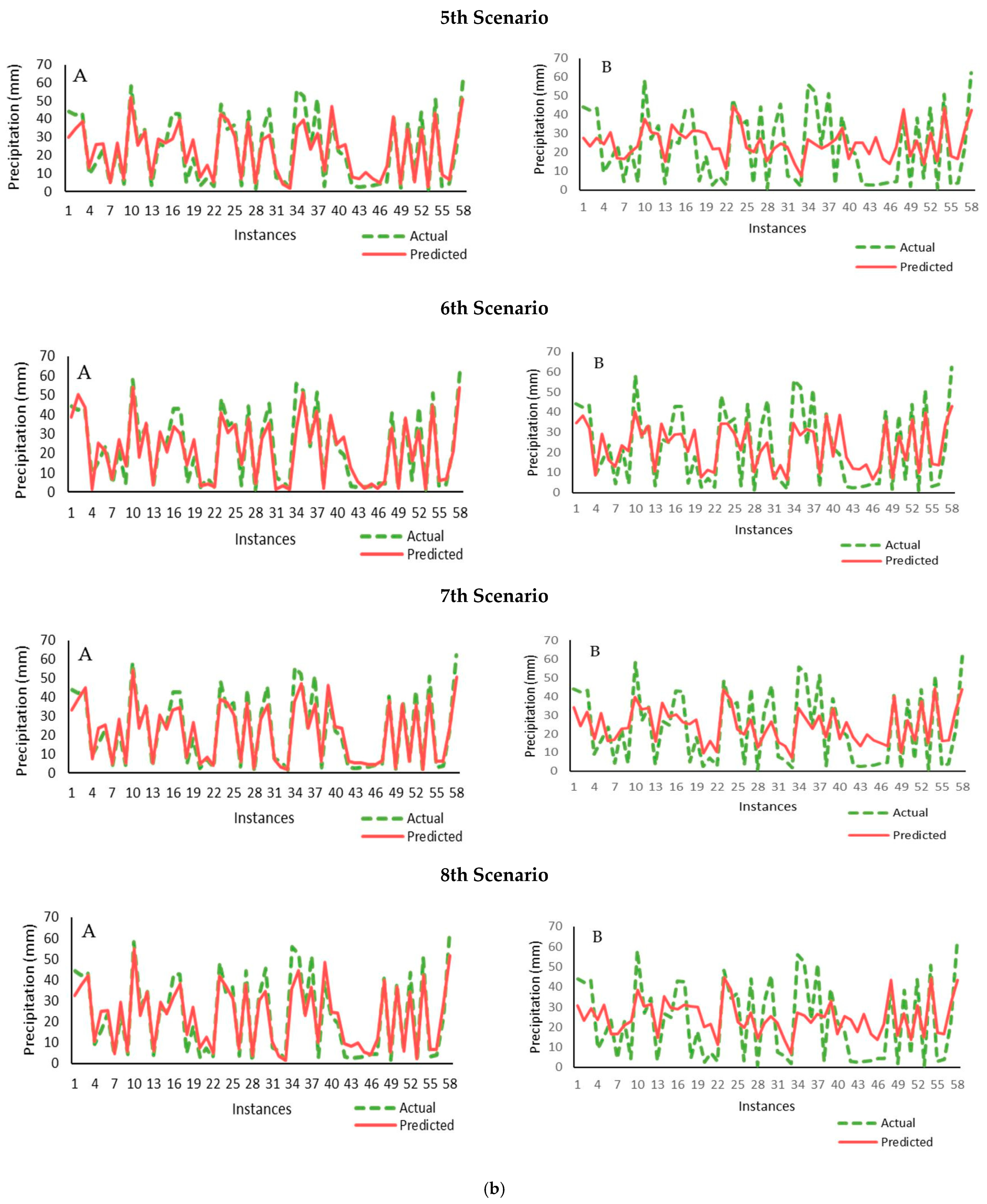
In the next step, a scatter diagram and a comparison were drawn for the best and worst models in each scenario, which can be seen in Figure 3 and Figure 4, respectively. The letters A show the performance of the best models, and the letters B show the worst models in each figure. A linear equation was drawn in scatter diagrams.
According to the scatter diagrams, in the third scenario (A), the equation line has the smallest distance with the points, indicating the best modeling. The γ value (i.e., slope value) is a significant parameter as it is a measure of the over- (γ > 1.0) or under-prediction (γ < 1.0) of the model compared to the observed data. In all scatter diagrams, the slope of the line is less than one, which indicates the under-prediction of the model in relation to the observational data.
In the third scatter diagram, the RF model has a slope equal to 0.889 and R2 equal to 0.912.
In the scatter diagrams, the vertical axis is the predicted data, and the horizontal axis is the actual precipitation data. In the profit diagrams, the vertical axis is the amount of precipitation, and the horizontal axis is an example of the amount of precipitation modeled.
3.2. Comparison Results of the Best Models of Each Scenario
In this step, the best model of each scenario, i.e., RFs, were selected to be compared with each other with the results presented in Table 5. The highest correlation coefficient calculated in the comparison is 0.9676, which belongs to the RF model scenario number 3, and the lowest belongs to the RF scenario number 5 with a value of 0.9425. All the models have shown good performance and have been able to predict the rainfall data with high accuracy. Each has obtained a high correlation coefficient of 0.94, which shows its strength in rainfall modeling and the lowest amount of all errors. The RF model of scenario No. 3 has been obtained, whose inputs include the monthly index, latitude, and distance of the stations from Lake Urmia and the Mediterranean Sea. This shows that these factors have the greatest impact on precipitation in the Lake Urmia basin. Also, this result was obtained in scenario three using four parameters under this scenario and the RF model. This is an advantage because even with a few parameters, it created an accurate model with low errors and high efficiency for predicting the rainfall pattern in the basin of Lake Urmia. Rainfall modeling in this basin can be utilized in many ways in various issues, including engineering and managing water resources in the Lake Urmia basin and more fundamental planning and planning for the future.
The best RF models of different scenarios are compared and sorted from the best to the worst in this table according to the correlation coefficient. This table shows that the best random forest is under scenario number 3. The other scenarios, from the best to the worst in comparison, are scenario number 7, 2, 4, 1, 8, and 6, and finally scenario 5.
The Nash–Sutcliffe efficiency in scenario number 3 in the random forest model was the highest and equal to 0.911. Considering the high value of the correlation coefficient in scenario number 3 in the random forest model and the low amount of errors, the random forest model of scenario number three is the best.
Another mode was investigated for all scenarios and models. In this method, the RF model was assumed to be out of reach for these data. Then, by comparing the correlation coefficient between all models in all scenarios, the next best model, after removing all RFs, is the KNN model from scenario six and with neighborhood 3. Under this scenario, this model has an acceptable and reasonable coefficient with only two monthly index inputs and the distance from Lake Urmia.
3.3. Zoning Map of Rainfall Changes
Zoning maps of rainfall changes for real data, data obtained from the best modeling, and data from the best scenario and model (RF scenario number 3) were drawn with Arc GIS software and compared with each other as shown in Figure 5a and b, respectively.
The IDW interpolation method was used to draw these maps to show the actual and predicted rainfall and ultimately shows that it has been able to model the precipitation accurately, and the result is very similar to the real precipitation map. Around Lake Urmia, especially east of the lake, there is very little precipitation in both real and modeled data. Shabestar and Miandoab stations have the lowest amount of precipitation.
4. Discussion
Today, rainfall modeling and forecasting are inseparable from engineering and water resources management. Therefore, both play an important role in managing water for irrigation, drinking water supply, and needs in the industrial and agricultural sectors. Precipitation in nature largely depends on spatial, temporal, and atmospheric variables, so it can be modeled by considering these parameters. Although various studies have been conducted to investigate precipitation in different parts of Iran, a comprehensive and detailed study and investigation have not been conducted in the Lake Urmia basin. In this study, the precipitation in the Lake Urmia basin was investigated completely and comprehensively with various models and spatial variables such as latitude and longitude, altitude, and station distance from the Mediterranean Sea and Lake Urmia. A relatively similar study was conducted in 2020 by Apaydin et al. [7]. In the coastal region of Turkey, they used deep learning methods to model precipitation. They used artificial intelligence methods such as Gaussian process regression, support vector regression, the Broyden–Fletcher–Goldfarb–Shanno artificial neural network, M5, random forest, and long short-term memory. The study shows that the amount of precipitation can be estimated and a distribution map can be drawn by using spatio-temporal data and the deep learning and GIS hybrid method at points where the measurement is not performed.
In another study conducted by Garai et al. [37] in 2024, algorithms based on complete ensemble empirical mode decomposition with adaptive noise combined with stochastic models like autoregressive integrated moving average and generalized autoregressive conditional heteroscedasticity; and machine learning techniques like a random forest, artificial neural network, support vector regression, and kernel ridge regression (KRR) have been proposed for predicting rainfall series. The proposed algorithms have been applied for predicting rainfall in three selected sub-divisions of India.
Another study was conducted by Parviz et al. [38] to improve hybrid models by using an ensemble of linear and non-linear models. They used precipitation data of two weather stations in Iran, namely Tabriz, East Azerbaijan, and Rasht, Gilan, over 1992–2019. Preprocessing configurations and each of the Gene Expression Programming (GEP), support vector regression (SVR), and Group Method of Data Handling (GMDH) models were used as in the traditional hybrid models. They were compared against the proposed hybrid models with a combination of all these three models. The results showed that Theil’s coefficient, which measures the inequality degree to which forecasts differ from observations, improved by 9% and 15% for SVR and GMDH relative to GEP for the Tabriz station. Generally, the representation of the non-linear models within the improved hybrid models showed better performance than the traditional hybrid models.
The most important feature of this study was the relatively accurate prediction of monthly rainfall without the need for measured rainfall amounts. In this research, for the first time, precipitation modeling was performed using an artificial intelligence algorithm and spatio-temporal variables in the Lake Urmia basin, especially the distance from the sea, and machine learning algorithms, and for the first time, the effect of distance from nearby seas on the basin’s precipitation is investigated. Considering the monthly time index for different stations, monthly rainfall was modeled using five machine learning models under eight scenarios. In general, by examining and analyzing the results, the following can be pointed out:
The eight defined scenarios were entered into the Weka software, and the five mentioned models were implemented in each of these scenarios. In GPR and SVR models, three sub-branches of kernel functions, namely PolyKernel, PUK, and RBFKernel, were investigated in all scenarios. After examining and modeling these functions, the PUK function had the best result in both models. Therefore, the results of this function were introduced as the best results of these two models. For the nearest neighbor model, neighborhoods from one to ten were examined for each model in each scenario, and the neighborhoods with the best results in each scenario were selected. Among all the eight defined scenarios, the RF model always had the best performance, had the highest correlation with the real data, and had the lowest error under different scenarios. It was chosen as the most suitable model, showing its high rainfall modeling ability.
In contrast, the GPR model always performed the worst. The RF model of scenario number three had the highest correlation. This indicates the high accuracy of this model under this particular scenario for the available data. In this scenario, the input data included the monthly index, latitude, and distance from Lake Urmia and the Mediterranean Sea. Accurate precipitation modeling using its four parameters can be a suitable and acceptable result in modeling science. Therefore, these four parameters can be considered the most important influencing factors on the precipitation in the Lake Urmia basin or the climatic conditions. It is notable that this model also has the least error. The zoning maps of the changes showed this clearly as well. The monthly index, which indicates the number of the month, is affected by different rainfall in different seasons in different months. The latitude indicates this basin’s general location, climate, and influence.
The distance of the stations from Lake Urmia can indicate the influence of the precipitation air masses formed from Lake Urmia itself. Finally, the distance from the Mediterranean Sea, which indicates the effect of the rain-producing air fronts caused by it in the basin of Lake Urmia, is an important and influential factor in the precipitation of this basin.
Future studies may consider using this method for other points as well or using other deep learning algorithms. On the other hand, in the future, the effect of the open seas on the rainfall of coastal areas in other parts of the world can be investigated.
5. Conclusions
The most important feature of this research is the demonstration of accurate precipitation modeling based on monthly precipitation data without the need to measure precipitation. That is, rainfall modeling and rainfall maps can be drawn by interpolation in the GIS environment using the RF model under scenario three, which has relatively high accuracy for the points where rainfall measurements are absent. Although studies have been conducted in different parts of Iran, a comprehensive and detailed study has not been carried out in the Lake Urmia basin. Therefore, in this study, precipitation in the Lake Urmia basin was investigated in a complete and comprehensive manner with various models, and spatial variables such as the latitude and longitude, altitude, and station distance from the Mediterranean Sea and Lake Urmia were used to model precipitation. This study also examined the effect of proximity of nearby seas on precipitation and subsequent fluctuations in the Lake Urmia basin.
Lastly, considering the monthly time index for different stations, monthly rainfall was modeled using five machine learning models (M5 decision tree model, RF (random forest) model, SVR model, GPR (Gaussian regression) model, and KNN model) under eight different scenarios. Among all the eight defined scenarios, the RF model always had the best performance and was able to have the highest correlation with the real data and the lowest error under different scenarios, and was thus chosen as the most suitable model. The RF model of scenario number three was the best among the eight scenarios and had the highest correlation with a rate of 0.968. In this scenario, the input data included four parameters: the monthly index, latitude, and distance from Lake Urmia and the Mediterranean Sea. The monthly index, which indicates the number of the month, is affected by different rainfall in different seasons in different months. The latitude indicates the general location and climate of this basin and its influence. The distance of the stations from Lake Urmia can indicate the influence of the precipitation air masses formed from Lake Urmia itself. Finally, the distance from the Mediterranean Sea, which indicates the impact of the rain-producing air fronts caused by it in the Lake Urmia basin, is an important and influential factor in the precipitation of this basin. Accurate modeling of precipitation using its four parameters can be a very suitable and acceptable result in modeling science. Therefore, these four parameters can be considered as the most important influencing factors on precipitation in the Lake Urmia basin or climatic conditions.
This new approach can now be used in the engineering, planning, and management of water resources in the Lake Urmia basin, and important steps can be taken to revive the lake. One major limitation of this study is that the results cannot be generalized to other basins due to the unique climatic conditions of each region. However, the same approach could be followed in other basins. Additionally, the complexity of the machine learning models and tools used in this study may make it difficult for non-experts to apply them, which is a disadvantage from an applicable standpoint.
Author Contributions
Conceptualization, M.T.S. and S.A.; methodology, M.T.S. and S.A.; software, S.A. and N.F.A.; validation, M.T.S.; formal analysis, M.S.; investigation, A.M.; data curation, S.A.; writing—original draft preparation, S.A. and N.F.A.; writing—review and editing, M.T.S. and A.M.; visualization, S.A. and N.F.A.; supervision, M.S.; project administration, M.T.S. and A.M.; funding acquisition, A.M. All authors have read and agreed to the published version of the manuscript.
Funding
This research received no external funding.
Data Availability Statement
Data are contained within the article.
Conflicts of Interest
The authors declare no conflicts of interest.
Appendix A
The Diebold–Mariano test is a statistical test used to compare the forecast accuracy of two competing forecasting models. Diebold–Mariano test results were obtained for each of the eight scenarios. If these values are lower than the critical value (here, 0.05), the null hypothesis will be rejected and it means that the two models have equal forecast accuracy, indicating that one model significantly outperforms the other. Table A1, Table A2, Table A3, Table A4, Table A5, Table A6, Table A7 and Table A8 show these values. All models and scenarios have the same forecast accuracy except the bold models, which are shown in each table.

Table A1.
First scenario p-value results for Diebold–Mariano test.
| GPR | KNN.IBK | M5 | Random.Forest | SVR.SMOREg | |
|---|---|---|---|---|---|
| GPR_GPR | 9.89078 × 10⁻⁵ | 0.008744 | 1.53123 × 10⁻⁷ | 5.86551 × 10⁻⁷ | |
| KNN-IBK | 9.89078 × 10⁻⁵ | 0.425019 | 0.000343249 | 0.242947779 | |
| M5 | 0.008743668 | 0.425019123 | 3.8851 × 10⁻⁵ | 0.128466214 | |
| Random forest | 1.53123 × 10⁻⁷ | 0.000343249 | 3.89 × 10⁻⁵ | 0.000255017 | |
| SVR-SMOREg | 5.86551 × 10⁻⁷ | 0.242947779 | 0.128466 | 0.000255017 |
Table A2.
Second scenario p-value results for Diebold–Mariano test.
| GPR | KNN.IBK | M5 | Random.Forest | SVR.SMOREg | |
|---|---|---|---|---|---|
| GPR_GPR | 1.36 × 10⁻⁶ | 2.6 × 10⁻⁵ | 1.96 × 10⁻¹⁰ | 5.05592 × 10⁻⁹ | |
| KNN-IBK | 1.36 × 10⁻⁶ | 0.502032 | 4.29 × 10⁻⁵ | 0.649852621 | |
| M5 | 2.6 × 10⁻⁵ | 0.502032 | 2.75 × 10⁻⁵ | 0.694082881 | |
| Random forest | 1.96 × 10⁻¹⁰ | 4.29 × 10⁻⁵ | 2.75 × 10⁻⁵ | 2.4385 × 10⁻⁵ | |
| SVR-SMOREg | 5.06 × 10⁻⁹ | 0.649853 | 0.694083 | 2.44 × 10⁻⁵ |
Table A3.
Third scenario p-value results for Diebold–Mariano test.
| GPR | KNN.IBK | M5 | Random.Forest | SVR.SMOREg | |
|---|---|---|---|---|---|
| GPR_GPR | 0.239647 | 3.41 × 10⁻⁸ | 8.16 × 10⁻¹¹ | 6.37 × 10⁻⁷ | |
| KNN-IBK | 0.239647 | 9.36 × 10⁻⁵ | 1.2 × 10⁻⁷ | 0.002914 | |
| M5 | 3.41 × 10⁻⁸ | 9.36 × 10⁻⁵ | 1.45 × 10⁻⁶ | 0.113727 | |
| Random forest | 8.16 × 10⁻¹¹ | 1.2 × 10⁻⁷ | 1.45 × 10⁻⁶ | 4.8 × 10⁻⁶ | |
| SVR-SMOREg | 6.37 × 10⁻⁷ | 0.002914 | 0.113727 | 4.8 × 10⁻⁶ |
Table A4.
Fourth scenario p-value results for Diebold–Mariano test.
| GPR | KNN.IBK | M5 | Random.Forest | SVR.SMOREg | |
|---|---|---|---|---|---|
| GPR_GPR | 0.029746 | 1.71 × 10⁻⁸ | 5.68 × 10⁻¹¹ | 4.14 × 10⁻⁶ | |
| KNN-IBK | 0.029746 | 0.005356 | 1.54 × 10⁻⁵ | 0.126692 | |
| M5 | 1.71 × 10⁻⁸ | 0.005356 | 2.65 × 10⁻⁵ | 0.018715 | |
| Random forest | 5.68 × 10⁻¹¹ | 1.54 × 10⁻⁵ | 2.65 × 10⁻⁵ | 9.59 × 10⁻⁶ | |
| SVR-SMOREg | 4.14 × 10⁻⁶ | 0.126692 | 0.018715 | 9.59 × 10⁻⁵ |
Table A5.
Fifth scenario p-value results for Diebold–Mariano test.
| GPR | KNN.IBK | M5 | Random.Forest | SVR.SMOREg | |
|---|---|---|---|---|---|
| GPR_GPR | 0.008865 | 8.35 × 10⁻⁹ | 4.02 × 10⁻¹¹ | 5.83 × 10⁻⁷ | |
| KNN-IBK | 0.008865 | 0.004905 | 7 × 10⁻⁵ | 0.24729 | |
| M5 | 8.35 × 10⁻⁹ | 0.004905 | 0.00328 | 0.00416 | |
| Random forest | 4.02 × 10⁻¹¹ | 7 × 10⁻⁵ | 0.00328 | 3.74 × 10⁻⁶ | |
| SVR-SMOREg | 5.83 × 10⁻⁷ | 0.24729 | 0.00416 | 3.74 × 10⁻⁶ |
Table A6.
Sixth scenario p-value results for Diebold–Mariano test.
| GPR | KNN.IBK | M5 | Random.Forest | SVR.SMOREg | |
|---|---|---|---|---|---|
| GPR_GPR | 7.7 × 10⁻⁶ | 0.012552 | 1.35 × 10⁻⁶ | 5.7 × 10⁻⁶ | |
| KNN-IBK | 7.7 × 10⁻⁶ | 0.010868 | 0.49152 | 0.015912 | |
| M5 | 0.012552 | 0.010868 | 0.003817 | 0.171806 | |
| Random forest | 1.35 × 10⁻⁶ | 0.49152 | 0.003817 | 0.003317 | |
| SVR-SMOREg | 5.7 × 10⁻⁶ | 0.015912 | 0.171806 | 0.003317 |
Table A7.
Seventh scenario p-value results for Diebold–Mariano test.
| GPR | KNN.IBK | M5 | Random.Forest | SVR.SMOREg | |
|---|---|---|---|---|---|
| GPR_GPR | 0.001948 | 0.005009 | 1.41 × 10⁻¹⁰ | 1.12 × 10⁻¹⁰ | |
| KNN-IBK | 0.001948 | 0.647415 | 3.27 × 10⁻⁵ | 0.01261 | |
| M5 | 0.005009 | 0.647415 | 3.03 × 10⁻⁵ | 0.138436 | |
| Random forest | 1.41 × 10⁻¹⁰ | 3.27 × 10⁻⁵ | 3.03 × 10⁻⁵ | 0.000128 | |
| SVR-SMOREg | 1.12 × 10⁻¹⁰ | 0.01261 | 0.138436 | 0.000128 |
Table A8.
Eighth scenario p-value results for Diebold–Mariano test.
| GPR | KNN.IBK | M5 | Random.Forest | SVR.SMOREg | |
|---|---|---|---|---|---|
| GPR_GPR | 0.048849 | 3.29 × 10⁻⁸ | 4.33 × 10⁻¹¹ | 1.07 × 10⁻⁷ | |
| KNN-IBK | 0.048849 | 0.006959 | 2.03 × 10⁻⁵ | 0.026509 | |
| M5 | 3.29 × 10⁻⁸ | 0.006959 | 6.34 × 10⁻⁵ | 0.052325 | |
| Random forest | 4.33 × 10⁻¹¹ | 2.03 × 10⁻⁵ | 6.34 × 10⁻⁵ | 4.3 × 10⁻⁶ | |
| SVR-SMOREg | 1.07 × 10⁻⁷ | 0.026509 | 0.052325 | 4.3 × 10⁻⁶ |
References
- Hasanalizadeh, N.; Mosaedi, A.; Zahiri, A.; Hosseinalizadeh, M. Modeling Spatio-Temporal Variation of Monthly Precipitation (Case Study: Golestan Province). J. Water Soil Conserv. 2014, 22, 251–269. [Google Scholar]
- Sattari, M.T.; RezazadehJoudi, A.; Nahrein, F. Monthly Rainfall Prediction using Artificial Neural Networks and M5 Model Tree (Case study: Station of AHAR). Phys. Geogr. Res. Q. 2014, 46, 247–260. [Google Scholar] [CrossRef]
- Zahedi Qara Aghaj, M.; Qavidel Rahimi, Y. Determining the Threshold of Drought and Calculating the Reliable Amount of Precipitation in the Watershed Stations of Lake Urmia Basin. Geogr. Res. 2007, 21. Available online: https://jrg.ut.ac.ir/article_18518.html?lang=en (accessed on 4 March 2024).
- Mohmadzadeh, K.; Feizizadeh, B. Modeling the Impacts of Urmia Lake Drought on Soil Salinity of Agricultural Lands in the Eastern Area of Fuzzy Object Based Image Analysis Approach. J. RS GIS Nat. Resour. 2017, 11, 56–72. [Google Scholar]
- Pham, Q.B.; Abba, S.I.; Usman, A.G.; Linh, N.T.T.; Gupta, V.; Malik, A.; Costache, R.; Vo, N.D.; Tri, D.Q. Potential of Hybrid Data-Intelligence Algorithms for Multi-Station Modelling of Rainfall. Water Resour. Manag. 2019, 33, 5067–5087. [Google Scholar] [CrossRef]
- Paul, R.K.; Paul, A.K.; Bhar, L.M. Wavelet-Based Combination Approach for Modeling Sub-Divisional Rainfall in India. Theor. Appl. Climatol. 2020, 139, 949–963. [Google Scholar] [CrossRef]
- Apaydin, H.; Sattari, M.T. Deep-Learning GIS Hybrid Approach in Precipitation Modeling Based on Spatio-Temporal Variables in the Coastal Zone of Turkey. Clim. Res. 2020, 81, 149–165. [Google Scholar] [CrossRef]
- De Oliveira, V.A.; Rodrigues, A.F.; Morais, M.A.V.; de Castro Nunes Santos Terra, M.; Guo, L.; de Mello, C.R. Spatiotemporal Modelling of Soil Moisture in an Atlantic Forest through Machine Learning Algorithms. Eur. J. Soil Sci. 2021, 72, 1969–1987. [Google Scholar] [CrossRef]
- Di Nunno, F.; Granata, F.; Pham, Q.B.; de Marinis, G. Precipitation Forecasting in Northern Bangladesh Using a Hybrid Machine Learning Model. Sustainability 2022, 14, 2663. [Google Scholar] [CrossRef]
- Wahla, S.; Kazmi, J.; Sharifi, A.; Shirazi, S.A.; Tariq, A.; Smith, H. Assessing Spatio-Temporal Mapping and Monitoring of Climatic Variability Using SPEI and RF Machine Learning Models. Geocarto Int. 2022, 38, 21. [Google Scholar] [CrossRef]
- Di Nunno, F.; Granata, F. Spatio-Temporal Analysis of Drought in Southern Italy: A Combined Clustering-Forecasting Approach Based on SPEI Index and Artificial Intelligence Algorithms. Stoch. Environ. Res. Risk Assess. 2023, 37, 2349–2375. [Google Scholar] [CrossRef]
- Ghebleh, M.; Jafarzadeh, A.; Ahmadi, M.P. Spatial-Temporal Changes of Precipitation in Urmia Lake Basin. In Proceedings of the International Conference on Sustainable Development With a focus on Agriculture, Environment and Tourism, Tabriz, Iran, 16 September 2015. [Google Scholar]
- Frank, E.; Hall, M.A.; Witten, I.H. The WEKA Workbench. In Data Mining; Morgan Kaufmann: Burlington, VT, USA, 2017; pp. 553–571. [Google Scholar] [CrossRef]
- Hall, M.; Frank, E.; Holmes, G.; Pfahringer, B.; Reutemann, P.; Witten, I.H. The WEKA Data Mining Software. ACM SIGKDD Explor. Newsl. 2009, 11, 10–18. [Google Scholar] [CrossRef]
- Quinlan, J.R. Learning with Continuous Classes. Aust. Jt. Conf. Artif. Intell. 1992, 92, 343–348. [Google Scholar]
- Quinlan, J.R. Induction of Decision Trees. Mach. Learn. 1986, 1, 81–106. [Google Scholar] [CrossRef]
- Falahi, M.; Varvani, H.; Golian, S. Rainfall Forecasting Using Regression Tree Model for Flood Control. In Proceedings of the 5th National Conference on Watershed Management and Soil and Water Resources Management, Kerman, Iran, 29 February 2012. [Google Scholar]
- Alberg, D.; Last, M.; Kandel, A. Knowledge Discovery in Data Streams with Regression Tree Methods. Wiley Interdisc. Rew. Data Min. Knowl. Discov. 2012, 2, 69–78. [Google Scholar] [CrossRef]
- Breiman, L. Random Forests. Mach. Learn. 2001, 45, 5–32. [Google Scholar] [CrossRef]
- Kulkarni, V.Y.; Sinha, P.K. Effective Learning and Classification Using Random Forest Algorithm. Int. J. Eng. Innov. Technol. 2014, 3, 267–273. [Google Scholar]
- Frankel, D.S. Model Driven Architecture: Applying MDA to Enterprise Computing; Wiley: Hoboken, NJ, USA, 2003; ISBN 9780471462279. [Google Scholar]
- Vapnik, V.N. Statistical Learning Theory; Wiley: Hoboken, NJ, USA, 1998; ISBN 978-0-471-03003-4. [Google Scholar]
- Chen, C.-C.; Wu, J.-K.; Lin, H.-W.; Pai, T.-P.; Fu, T.-F.; Wu, C.-L.; Tully, T.; Chiang, A.-S. Visualizing Long-Term Memory Formation in Two Neurons of the Drosophila Brain. Science 2012, 335, 678–685. [Google Scholar] [CrossRef]
- Cristianini, N.; Shawe-Taylor, J. An Introduction to Support Vector Machines and Other Kernel-Based Learning Methods; Cambridge University Press: Cambridge, UK, 2000; ISBN 9780521780193. [Google Scholar]
- Omran, B.A.; Chen, Q.; Jin, R. Comparison of Data Mining Techniques for Predicting Compressive Strength of Environmentally Friendly Concrete. J. Comput. Civ. Eng. 2016, 30, 4016029. [Google Scholar] [CrossRef]
- Cheng, M.-Y.; Huang, C.-C.; Roy, A.F. Van Predicting Project Success in Construction Using an Evolutionary Gaussian Process Inference Model. J. Civ. Eng. Manag. 2013, 19, S202–S211. [Google Scholar] [CrossRef]
- Pal, M.; Deswal, S. Modelling Pile Capacity Using Gaussian Process Regression. Comput. Geotech. 2010, 37, 942–947. [Google Scholar] [CrossRef]
- Rezazadeh Joudi, A.; Sattari, M.T. Performance Evaluation of Data-Driven Methods in Mashhad Monthly Rainfall Modelling. Iran. Water Res. J. 2017. Available online: https://iwrj.sku.ac.ir/article_10568.html?lang=en (accessed on 4 March 2024).
- Wu, X.; Kumar, V.; Ross, Q.J.; Ghosh, J.; Yang, Q.; Motoda, H.; McLachlan, G.J.; Ng, A.; Liu, B.; Yu, P.S.; et al. Top 10 Algorithms in Data Mining. Knowl. Inf. Syst. 2008, 14, 1–37. [Google Scholar] [CrossRef]
- Fadaei Kermani, E.; Khanjani, M.; Barani, G. Application of K-Nearest Neighbor Algorithm in Drought Monitoring Based on Standard Precipitation Index (SPI) of Bam City. Int. Bull. Water Resour. Dev. 2014, 131. Available online: https://www.magiran.com/paper/1399321/application-of-k-nearest-neighbor-algorithm-in-drought-monitoring-based-on-the-standard-precipitation-index-a-case-study-of-city-of-bam-southeastern-iran?lang=en (accessed on 4 March 2024).
- Jagtap, S.S.; Lall, U.; Jones, J.W.; Gijsman, A.J.; Ritchie, J.T. Dynamic Nearest-Neighbor Method for Estimating Soil Water Parameters. Trans. Am. Soc. Agric. Eng. 2004, 47, 1437–1444. [Google Scholar] [CrossRef]
- Nash, J.E.; Sutcliffe, J. V River Flow Forecasting through Conceptual Models Part I—A Discussion of Principles. J. Hydrol. 1970, 10, 282–290. [Google Scholar] [CrossRef]
- Gikas, G.; Yiannakopoulou, T.; Tsihrintzis, V. Modeling of Non-Point Source Pollution in a Mediterranean Drainage Basin. Environ. Model. Assess. 2006, 11, 219–233. [Google Scholar] [CrossRef]
- Tsihrintzis, V.; Hamid, R. Urban Stormwater Quantity/Quality Modeling Using the SCS Method and Empirical Equations. JAWRA J. Am. Water Resour. Assoc. 2007, 33, 163–176. [Google Scholar] [CrossRef]
- Tsihrintzis, V.A.; Hamid, R. Runoff Quality Prediction from Small Urban Catchments Using SWMM. Hydrol. Process. 1998, 12, 311–329. [Google Scholar] [CrossRef]
- Boskidis, I.; Gikas, G.D.; Pisinaras, V.; Tsihrintzis, V.A. Spatial and Temporal Changes of Water Quality, and SWAT Modeling of Vosvozis River Basin, North Greece. J. Environ. Sci. Health Part A 2010, 45, 1421–1440. [Google Scholar] [CrossRef] [PubMed]
- Garai, S.; Paul, R.K.; Yeasin, M.; Roy, H.S.; Paul, A.K. Machine Learning Algorithms for Predicting Rainfall in India. Curr. Sci. 2024, 126, 360–367. [Google Scholar]
- Parviz, L.; Rasouli, K.; Torabi Haghighi, A. Improving Hybrid Models for Precipitation Forecasting by Combining Nonlinear Machine Learning Methods. Water Resour. Manag. 2023, 37, 3833–3855. [Google Scholar] [CrossRef]
Figure 1.
Geographical location of Lake Urmia basin and selected meteorological stations.

Figure 2.
Total monthly precipitation graph of each station compared to basin average.

Figure 3.
(a) Scatter diagram of the best and worst models. (b) Scatter diagram of the best and worst models.
Figure 3.
(a) Scatter diagram of the best and worst models. (b) Scatter diagram of the best and worst models.


Figure 4.
(a) Comparison diagram of the best and worst models. (b) Comparison diagram of the best and worst models.
Figure 4.
(a) Comparison diagram of the best and worst models. (b) Comparison diagram of the best and worst models.


Figure 5.
Precipitation zoning is based on real data and modeled by best model. (a) Real data map. (b) Modeled data map.
Figure 5.
Precipitation zoning is based on real data and modeled by best model. (a) Real data map. (b) Modeled data map.

Table 1.
Monthly precipitation characteristics for each station (General Directorate of Meteorology of Tabriz and Urmia).
Table 1.
Monthly precipitation characteristics for each station (General Directorate of Meteorology of Tabriz and Urmia).
| Stations | Min Precip (mm) | Max Precip (mm) | Mean Precip (mm) | Standard Deviation of Precip Data (mm) | Longitude (Degree) | Latitude (Degree) | Height (m) | Distance from the Lake (km) | Distance from the Mediterranean Sea | Data Period (Year) |
|---|---|---|---|---|---|---|---|---|---|---|
| Salmas | 7.073 | 44.553 | 20.431 | 12.720 | 44°51′0″ | 38°13′0″ | 1339 | 13.821 | 787.542 | 2001–2021 |
| Urmia | 2.634 | 60.300 | 27.932 | 18.814 | 45°2′59″ | 37°32′57″ | 1328 | 18.936 | 791.510 | 1951–2021 |
| Oshnavieh | 2.825 | 62.246 | 33.057 | 22.711 | 45°7′59″ | 37°2′59″ | 1416 | 28.727 | 796.632 | 2006–2021 |
| Naghdeh | 1.257 | 54.865 | 26.777 | 19.512 | 45°25′0″ | 36°57′0″ | 1307 | 17.655 | 821.696 | 2001–2021 |
| Mahabad | 0.975 | 62.115 | 32.175 | 23.680 | 45°43′0″ | 36°45′0″ | 1352 | 31.101 | 849.505 | 1985–2021 |
| Bukan | 2.159 | 51.994 | 28.680 | 20.551 | 46°13′59″ | 36°31′59″ | 1386 | 70.345 | 897.398 | 2005–2021 |
| Shahin Dej | 2.583 | 52.415 | 25.494 | 17.070 | 46°31′0″ | 36°37′0″ | 1395 | 81.010 | 921.399 | 2006–2021 |
| Miandoab | 0.940 | 50.131 | 22.669 | 16.523 | 46°9′1″ | 36°58′0″ | 1270 | 33.767 | 886.704 | 2002–2021 |
| Malekan | 0.829 | 39.365 | 21.523 | 14.333 | 46°5′41″ | 37°10′9″ | 1299 | 21.836 | 880.945 | 2008–2021 |
| Maragheh Airport | 1.152 | 55.876 | 24.223 | 17.729 | 46°8′46″ | 37°20′51″ | 1342 | 13.349 | 885.618 | 1983–2021 |
| Ajabshir | 0.744 | 34.731 | 16.566 | 12.016 | 45°51′54″ | 37°30′32″ | 1310 | 5.205 | 861.638 | 2013–2021 |
| Sahand | 3.157 | 42.309 | 18.353 | 12.061 | 46°9′24″ | 37°55′25″ | 1695 | 42.879 | 891.668 | 1985–2021 |
| Tabriz Airport | 3.604 | 51.602 | 23.567 | 14.662 | 46°14′1″ | 38°7′20″ | 1345 | 53.547 | 900.387 | 1951–2021 |
| Marand | 8.386 | 62.576 | 31.873 | 17.949 | 45°46′13″ | 38°22′53″ | 1548 | 34.519 | 864.101 | 2000–2021 |
| Shabestar | 2.272 | 35.981 | 18.682 | 11.396 | 45°41′0″ | 38°10′18″ | 1385 | 9.632 | 853.635 | 2012–2021 |
| Bonab | 1.507 | 51.769 | 21.295 | 15.523 | 46°3′7″ | 37°22′11″ | 1281 | 5.061 | 879.406 | 1999–2021 |
Table 2.
List of parameters and abbreviations used in the model.
| Abbreviation | Parameter |
|---|---|
| M | Month Index |
| DM | Distance to the Mediterranean Sea |
| DU | Distance to Lake Urmia |
| X | Longitude |
| Y | Latitude |
| Z | Altitude |
Table 3.
Different scenarios with input parameters and their selection method and Relief attribute Eval and Correlation Matrix method with parameters.
Table 3.
Different scenarios with input parameters and their selection method and Relief attribute Eval and Correlation Matrix method with parameters.
| Scenario | Input | Scenario Selection Method | Parameter | Rated Features | Correlation |
|---|---|---|---|---|---|
| 1 | M, Y | Correlation Matrix | M | 0.072 | −0.262 |
| 2 | M, Y, DU | Correlation Matrix | DU | −0.013 | 0.092 |
| 3 | M, Y, DU, DM | Correlation Matrix | Y | −0.010 | −0.103 |
| 4 | M, Y, DU, DM, X | Correlation Matrix | Z | −0.009 | 0.021 |
| 5 | M, Y, DU, DM, X, Z | Correlation Matrix | X | −0.008 | −0.067 |
| 6 | M, DU | Relief | DM | −0.008 | −0.074 |
| 7 | M, DU, Y, Z | Relief | |||
| 8 | M, DU, Y, Z, X | Relief |
Table 4.
Scenarios and models with their evaluation criteria of R, NS, MAE, and RMSE.
| Scenario | Model | R | NS | MAE (mm) | RMSE (mm) |
|---|---|---|---|---|---|
| 1 | RF | 0.959 | 0.901 | 4.055 | 5.979 |
| SVR | 0.919 | 0.816 | 6.555 | 8.156 | |
| M5 | 0.918 | 0.768 | 7.408 | 9.156 | |
| KNN | 0.907 | 0.796 | 6.712 | 8.600 | |
| GPR | 0.882 | 0.693 | 9.205 | 10.540 | |
| 2 | RF | 0.964 | 0.902 | 4.246 | 5.957 |
| M5 | 0.919 | 0.772 | 7.312 | 9.093 | |
| SVR | 0.917 | 0.789 | 7.133 | 8.748 | |
| KNN | 0.912 | 0.798 | 6.827 | 8.558 | |
| GPR | 0.845 | 0.601 | 10.684 | 12.012 | |
| 3 | RF | 0.968 | 0.911 | 4.033 | 5.666 |
| M5 | 0.929 | 0.783 | 7.162 | 8.867 | |
| SVR | 0.866 | 0.711 | 8.581 | 10.227 | |
| KNN | 0.757 | 0.505 | 11.436 | 13.382 | |
| GPR | 0.738 | 0.455 | 12.495 | 14.044 | |
| 4 | RF | 0.961 | 0.892 | 4.737 | 6.249 |
| M5 | 0.929 | 0.783 | 7.162 | 8.867 | |
| SVR | 0.829 | 0.651 | 9.309 | 11.249 | |
| KNN | 0.747 | 0.557 | 9.838 | 12.659 | |
| GPR | 0.693 | 0.406 | 13.032 | 14.666 | |
| 5 | RF | 0.943 | 0.850 | 5.840 | 7.359 |
| M5 | 0.929 | 0.786 | 7.137 | 8.809 | |
| SVR | 0.816 | 0.625 | 9.717 | 11.658 | |
| KNN | 0.747 | 0.557 | 9.838 | 12.659 | |
| GPR | 0.661 | 0.372 | 13.430 | 15.080 | |
| 6 | RF | 0.943 | 0.878 | 5.036 | 6.653 |
| KNN | 0.936 | 0.858 | 6.107 | 7.176 | |
| SVR | 0.906 | 0.780 | 7.253 | 8.921 | |
| M5 | 0.903 | 0.738 | 8.012 | 9.743 | |
| GPR | 0.853 | 0.650 | 9.554 | 11.258 | |
| 7 | RF | 0.966 | 0.910 | 4.170 | 5.680 |
| SVR | 0.923 | 0.803 | 7.034 | 8.444 | |
| M5 | 0.889 | 0.722 | 8.067 | 10.033 | |
| KNN | 0.855 | 0.696 | 8.674 | 10.493 | |
| GPR | 0.824 | 0.570 | 11.116 | 12.474 | |
| 8 | RF | 0.957 | 0.886 | 5.004 | 6.418 |
| M5 | 0.924 | 0.776 | 7.289 | 8.998 | |
| SVR | 0.859 | 0.693 | 8.954 | 10.550 | |
| KNN | 0.747 | 0.557 | 9.838 | 12.659 | |
| GPR | 0.716 | 0.430 | 12.805 | 14.362 |
Table 5.
The best and worst models with respect to R, MAE, RMSE, and NS criteria.
| Best Model | RF | RF | RF | RF | RF | RF | RF | RF | Max | Min |
|---|---|---|---|---|---|---|---|---|---|---|
| Scenario | 3 | 7 | 2 | 4 | 1 | 8 | 6 | 5 | ||
| R | 0.968 | 0.966 | 0.964 | 0.961 | 0.959 | 0.957 | 0.943 | 0.943 | 0.968 | 0.943 |
| NS | 0.911 | 0.910 | 0.902 | 0.892 | 0.901 | 0.886 | 0.878 | 0.850 | 0.911 | 0.850 |
| MAE (mm) | 4.033 | 4.170 | 4.246 | 4.737 | 4.055 | 5.004 | 5.036 | 5.840 | 5.840 | 4.033 |
| RMSE (mm) | 5.666 | 5.680 | 5.957 | 6.249 | 5.979 | 6.418 | 6.653 | 7.359 | 7.359 | 5.666 |
Disclaimer/Publisher’s Note: The statements, opinions and data contained in all publications are solely those of the individual author(s) and contributor(s) and not of MDPI and/or the editor(s). MDPI and/or the editor(s) disclaim responsibility for any injury to people or property resulting from any ideas, methods, instructions or products referred to in the content. |
© 2024 by the authors. Licensee MDPI, Basel, Switzerland. This article is an open access article distributed under the terms and conditions of the Creative Commons Attribution (CC BY) license (https://creativecommons.org/licenses/by/4.0/).
Share and Cite
MDPI and ACS Style
Arbabi, S.; Sattari, M.T.; Attar, N.F.; Milewski, A.; Sakizadeh, M. Precipitation Modeling Based on Spatio-Temporal Variation in Lake Urmia Basin Using Machine Learning Methods. Water 2024, 16, 1246. https://doi.org/10.3390/w16091246
AMA Style
Arbabi S, Sattari MT, Attar NF, Milewski A, Sakizadeh M. Precipitation Modeling Based on Spatio-Temporal Variation in Lake Urmia Basin Using Machine Learning Methods. Water. 2024; 16(9):1246. https://doi.org/10.3390/w16091246
Chicago/Turabian StyleArbabi, Sajjad, Mohammad Taghi Sattari, Nasrin Fathollahzadeh Attar, Adam Milewski, and Mohamad Sakizadeh. 2024. "Precipitation Modeling Based on Spatio-Temporal Variation in Lake Urmia Basin Using Machine Learning Methods" Water 16, no. 9: 1246. https://doi.org/10.3390/w16091246
Note that from the first issue of 2016, this journal uses article numbers instead of page numbers. See further details here.