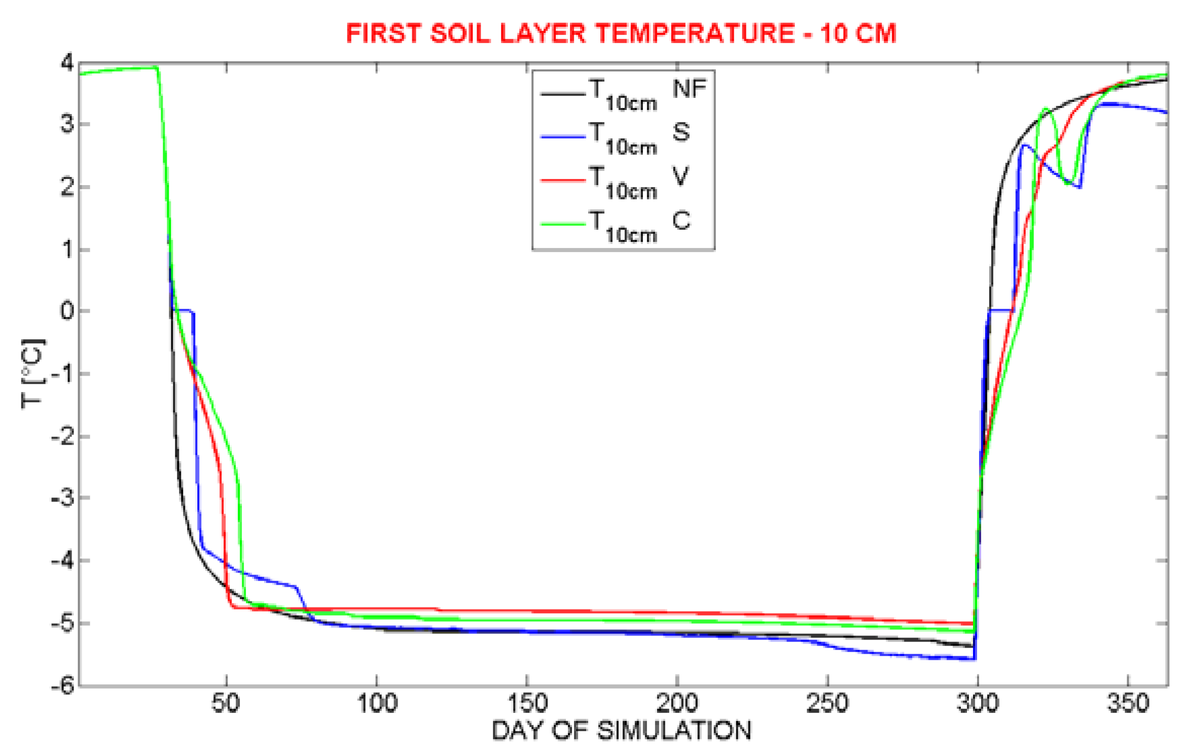
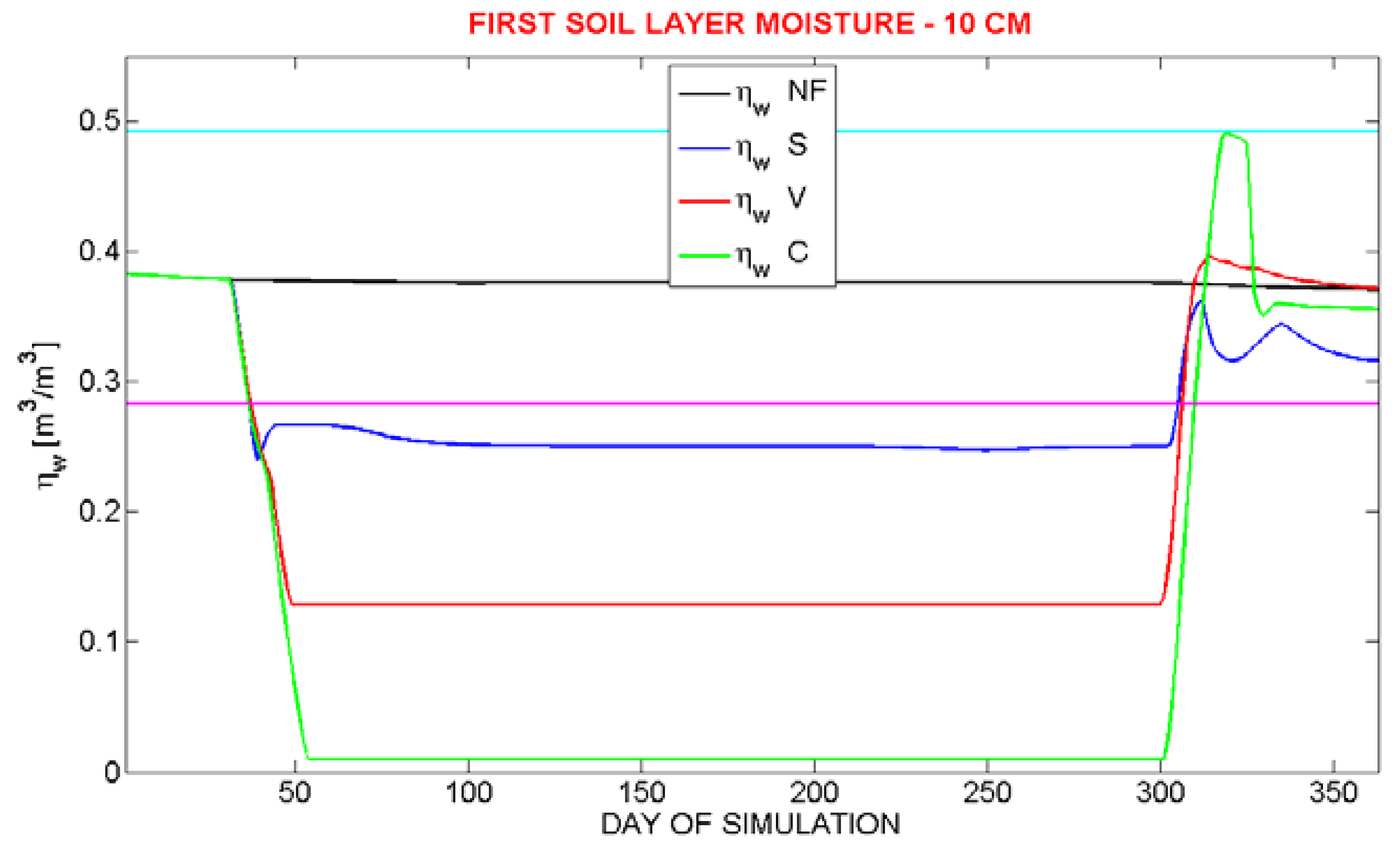
The results (
Figure 4 and
Figure 5) show that the model is able to reproduce the physical processes of both freezing and thawing using all three parameterizations above mentioned. In particular,
Figure 4 shows the warming of the layer affected by freezing with respect to ‘no freezing’ (“NF”) case (
i.e., when freezing is not activated), due to the latent heat release, while
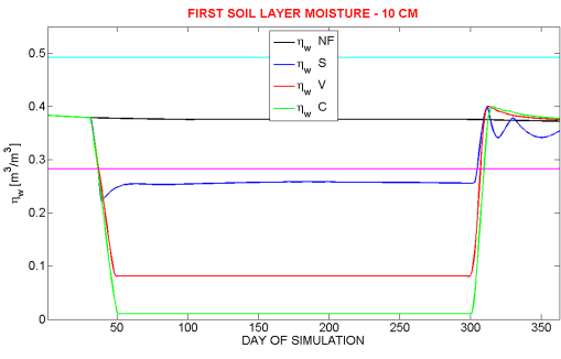
Figure 5 shows the decrease of the liquid water content
ηw during the freezing period. The warming of the layer in which ice forms is proportional to the quantity of ice present in the soil: this fact is not surprising, as the heating is linked to the latent heat release. In this sense, V and C parameterizations simulate the warmest temperatures and the biggest ice quantity.
Figure 4.
Simulated soil temperature in the 10 cm soil layer.
Figure 5.
Simulated soil moisture in the 10 cm soil layer. The cyan line is the porosity ηs, the pink line is the wilting point ηwi.
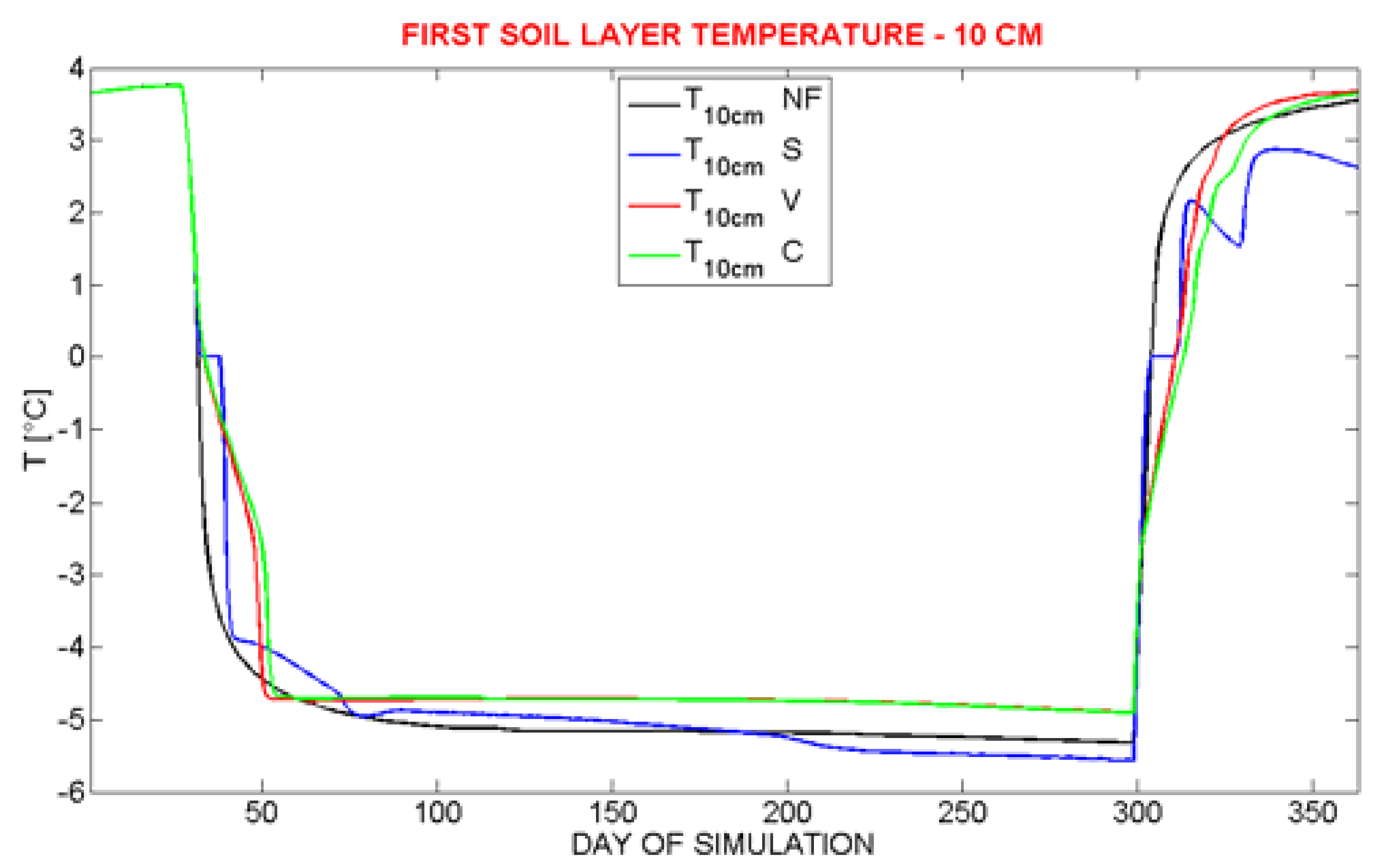
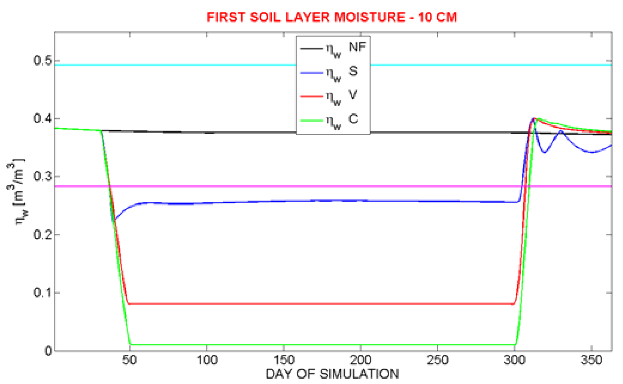
5..1 Numerical Instability during the Thawing Phase
Figure 4 and
Figure 5 show soil temperature and soil moisture oscillations during the thawing phase. This is due to two main factors: the first is that precipitation begins during the thawing period; the second is related to numerical instability, especially for the parameterization C.
Inspection of this problem revealed that the numerical part of this instability is caused by a single term.
In fact, the soil moisture is calculated from the conservation equation:
where
qwz is the soil water flux.
In this equation, the soil water flux, responsible for the above-mentioned numerical instability, is expressed by the following equation implemented in the UTOPIA model [
10]:
The first term on the right-hand-side of the equation is the soil water flux, related to the humidity gradient. This flux depends on the hydraulic diffusivity of liquid water Dwη and from the hydraulic diffusivity of water vapor Dvη. The second term is the water flux due to gravitational drainage, while the last one is the water vapor flux due to the temperature gradient.
In particular, the term responsible of numeric instability of soil moisture and temperature is the water vapor flux due to humidity gradient (
). Niu
et al. [
11] showed that this flux can be considered negligible for values of volumetric water content larger than 0.06 m
3/m
3. For this reason, the water vapor hydraulic diffusivity in the equation of soil water vertical flux has been set to zero for
ηw > 0.06 m
3/m
3, leading to a noticeable reduction of the instability (
Figure 6 and
Figure 7).
Figure 6.
Soil temperature in the 10 cm soil layer (as for
Figure 4) for the simulation performed when the water vapor hydraulic diffusivity is set to zero.
Figure 6.
Soil temperature in the 10 cm soil layer (as for
Figure 4) for the simulation performed when the water vapor hydraulic diffusivity is set to zero.
Figure 7.
Soil moisture in the 10 cm soil layer (as for
Figure 5) for the simulation performed when the water vapor hydraulic diffusivity is set to zero
Figure 7.
Soil moisture in the 10 cm soil layer (as for
Figure 5) for the simulation performed when the water vapor hydraulic diffusivity is set to zero
5.2. The Problem of Water Overproduction during Soil Freezing
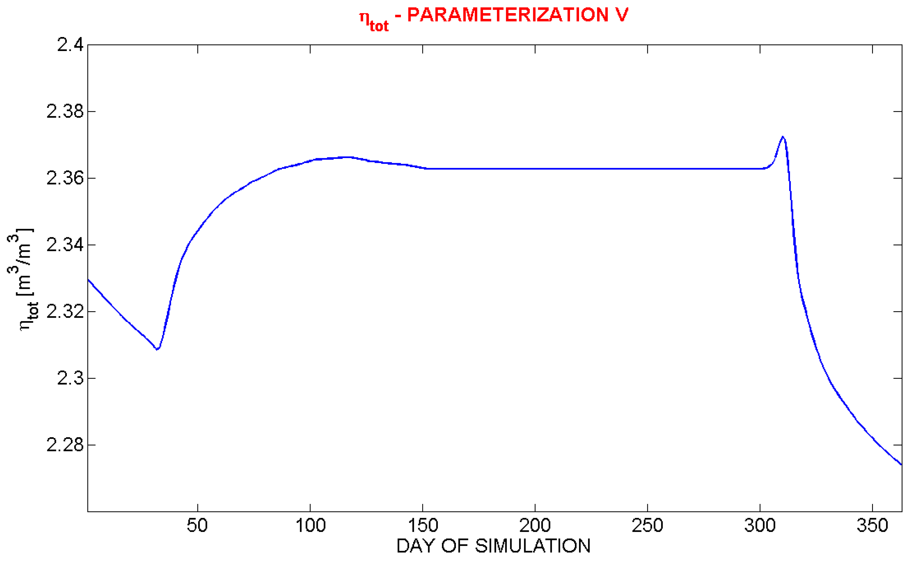
A second relevant problem encountered during the sensitivity tests concerning the phase change of water in the soil is the lack of conservation of the total soil water mass. This fact appears evident by considering the total volumetric water content (water and ice) in all model soil layers considered in a certain simulation.
In the ηTOT calculation, we considered the water density equal to 999.8 kg/m3 and the ice density equal to 917.0 kg/m3.
Figure 8 shows
ηTOT values corresponding to the simulation referring to
Figure 6 and
Figure 7. It is evident that, during the period of the soil freezing, the increase of
ηTOT is not justified on the basis of considerations related to hydrological soil balance. In fact, in the freezing period, there is no precipitation, and the transpiration stops because the temperatures drop below 0 °C, thus minimizing also the evaporation. Considering also the drainage from the bottom layer, a decrease, and not an increase, of total water content may be considered realistic.
Several analyses have shown that the term responsible of the observed water overproduction is the liquid water flux due to the humidity gradient (). This last term describes capillarity. In fact, when the soil starts to freeze, capillarity takes place because the ice formed in the soil occupies part of the soil pores volume.
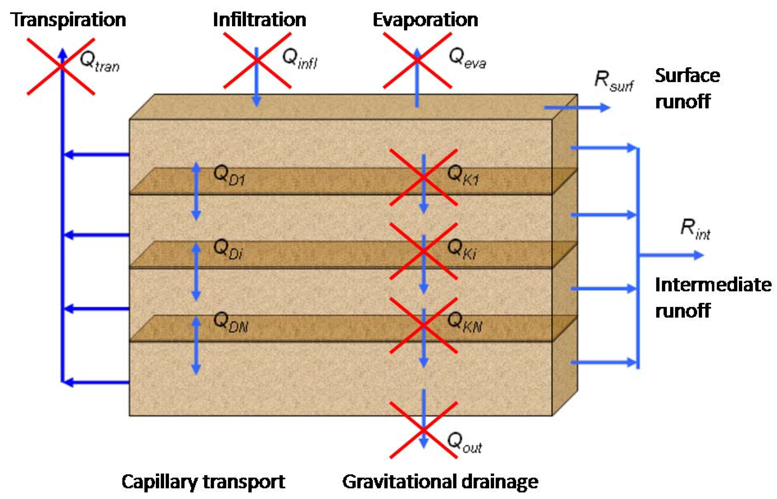
To demonstrate the relation between the water overproduction and the capillarity, we set all terms of the hydrological balance equation to zero, except this flux. If only surface and intermediate runoff are allowed (
Figure 9), an unreasonable increase of
ηtot is still present.
Figure 8.
ηtot trend for the simulation with synthetic data.
Figure 8.
ηtot trend for the simulation with synthetic data.
Figure 9.
Representation of the moisture fluxes between the different soil layers and the external environment. During the sensitivity test discussed in
Section 5.2, transpiration evaporation, infiltration and gravitational drainage have been set to zero.
Figure 9.
Representation of the moisture fluxes between the different soil layers and the external environment. During the sensitivity test discussed in
Section 5.2, transpiration evaporation, infiltration and gravitational drainage have been set to zero.
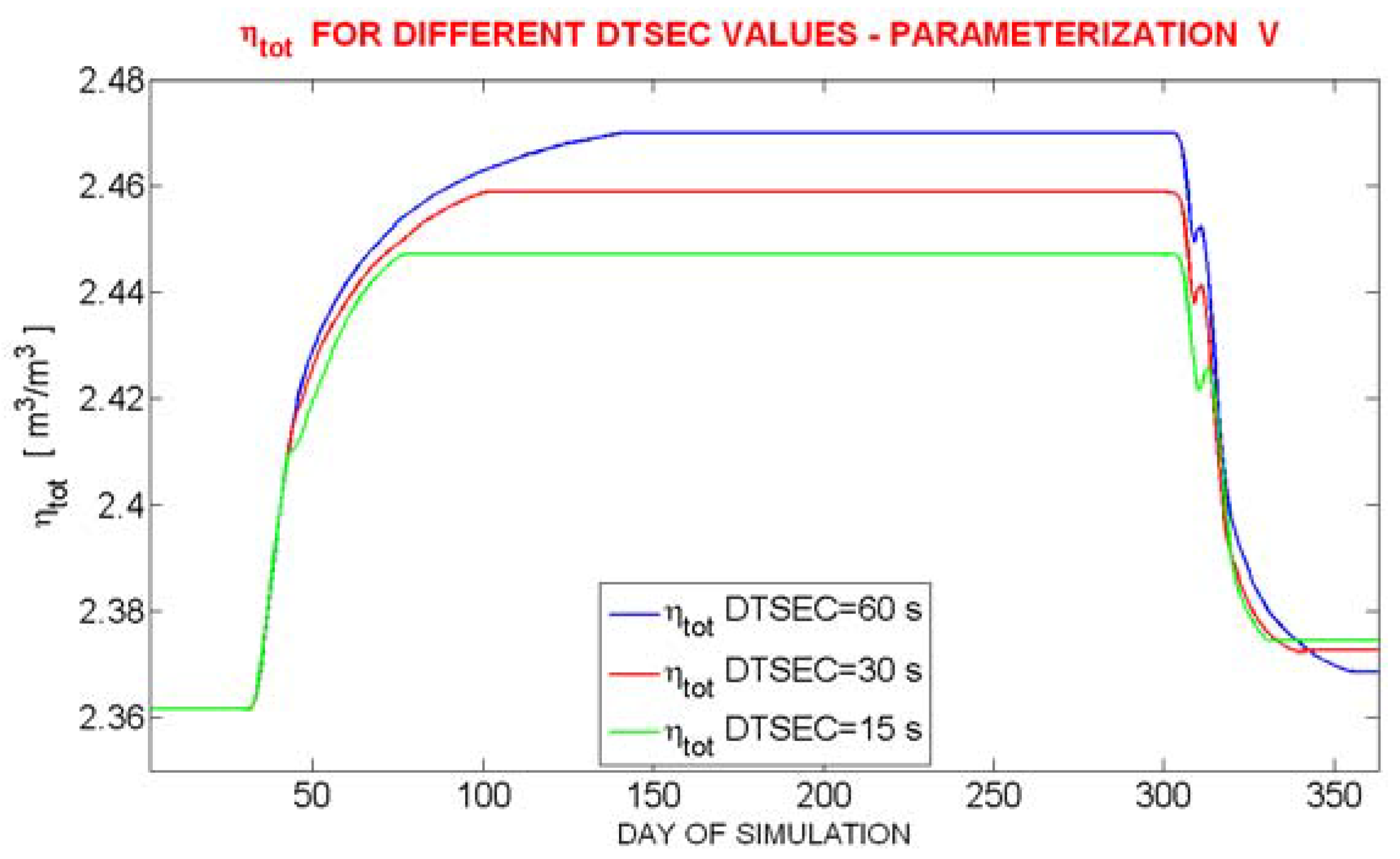
This behavior has been identified as a problem of numeric instability due to very fast variation of volumetric water content in the soil layers during the water-ice phase change. A reduction of the integration time-step in the UTOPIA model has resulted in a decrease of the water overproduction, as shown in
Figure 10. However, this approach for the solution of this problem cannot be adopted because it requires a very long computing time for the simulations.
Figure 10.
η tot trends evaluated in the sensitivity test summarized in
Figure 9. The three simulations have been executed using three different time step (DTSEC) values. The numerical convergence toward a constant value is just slightly shown. The complete numerical convergence would have been reached shorter values of DTSEC, however this is not shown because it requires too large a computation time.
An alternative approach has been adopted considering for each time-step the calculation of two variables for ηtot (in units of volumetric water content). The first one, called ηtot;correct, conserves the water mass during the freezing, while the second variable, called ηtot;effective, does not conserve the water mass.
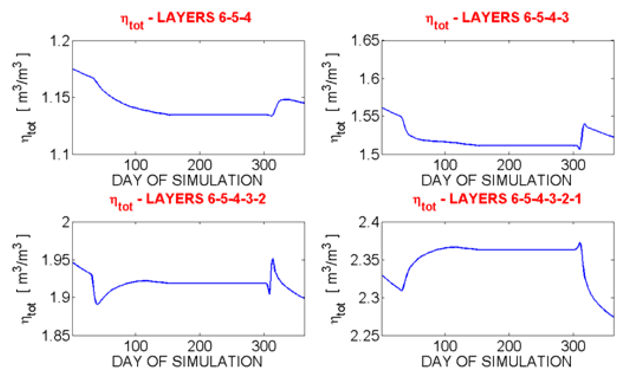
Simulation results show (
Figure 11 and
Figure 12) that the physically and hydrologically unreasonable increment of the total VSWC occur in presence of a water flux, due to the gradient humidity, towards soil layers with a significant ice production (
ηi > 0.01 m
3/m
3). Thus
ηtot begin to increase when the total VSWC of the second layer, where the volumetric ice content is greater than 0.01 m
3/m
3, is considered.
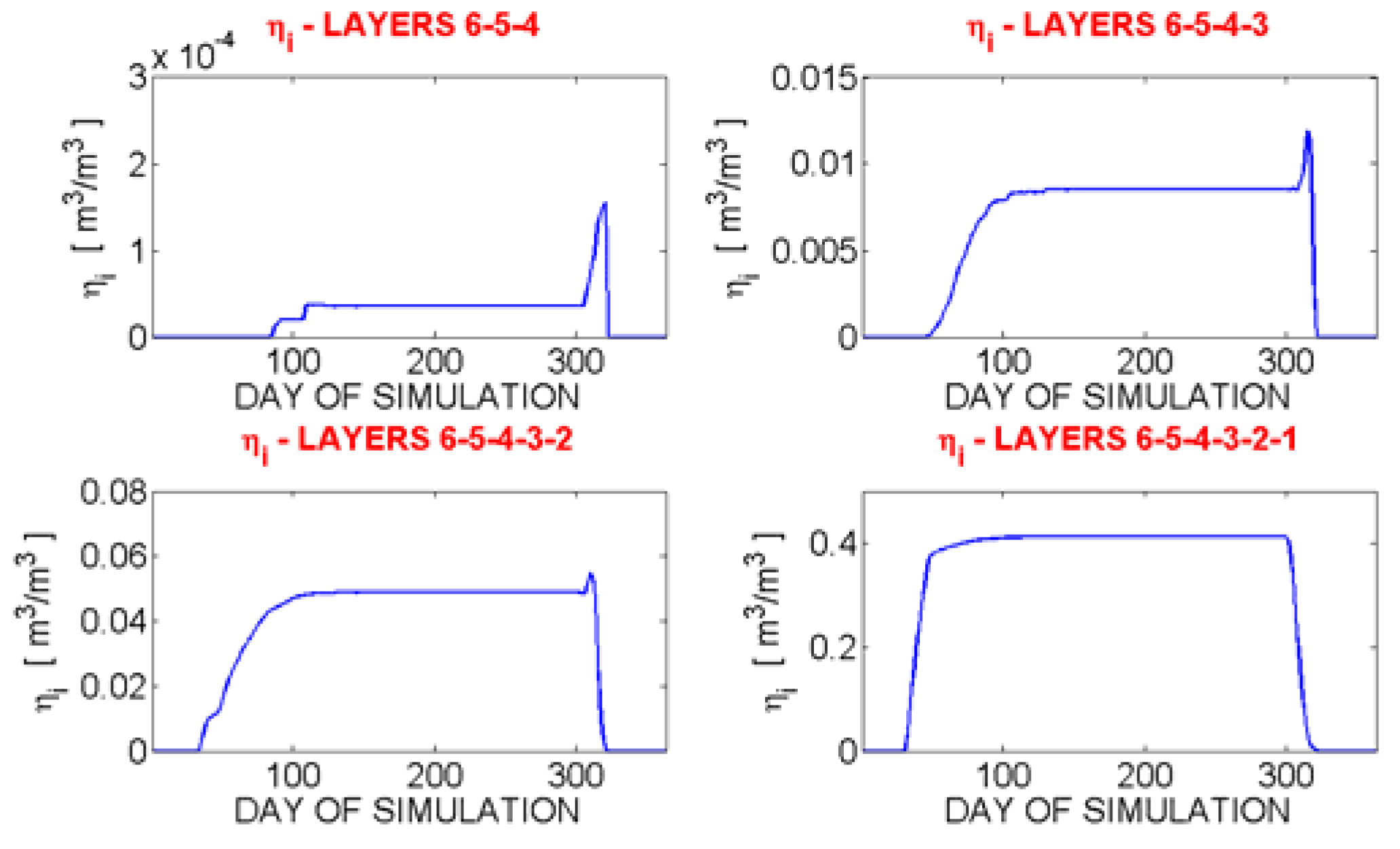
Figure 11.
ηtot trend relative to the sensitivity test summarized in
Figure 9, considering: the three deepest soil layers (top left), the four deepest soil layers (top right), the five deepest soil layers (bottom left), and all soil layers (bottom right).
Figure 11.
ηtot trend relative to the sensitivity test summarized in
Figure 9, considering: the three deepest soil layers (top left), the four deepest soil layers (top right), the five deepest soil layers (bottom left), and all soil layers (bottom right).
Figure 12.
ηi (volumetric ice content) trends relative to the sensitivity test summarized in
Figure 9, for the fourth layer (top left), the third layer (top right), second layer (bottom left) and first layer (bottom right).
Figure 12.
ηi (volumetric ice content) trends relative to the sensitivity test summarized in
Figure 9, for the fourth layer (top left), the third layer (top right), second layer (bottom left) and first layer (bottom right).
At the beginning of each time step, the quantity
ηi,tot,
i.e., the total volumetric ice content in all soil layers, is calculated. If
ηi,tot is greater than the minimum value 0.01 m
3/m
3 (
i.e., if there is a significant quantity of ice in soil), the variable
ηtot,correct is computed by setting to zero the hydraulic diffusivity (
Dwη= 0), in order to neglect the water fluxes among the soil layers due to the humidity gradient. In this way, the total VSWC (
η’w+η’i) of each layer contributes to conserve the total VSWC. Thus, the variable
ηtot;correct is calculated as:
at the same time, the total VSWC of all soil layers
ηtot,effective is calculated by accounting the true hydraulic diffusivity (
Dwη≠ 0) and it does not conserve the total VSWC:
At this point, as stated before, among all soil layers, those who do not conserve the total VSWC possess a significant ice production. Thus, the following correction on
ηw is performed only in those soil layers in which the volumetric ice content is significant (with
ηi > 0.01 m
3/m
3):
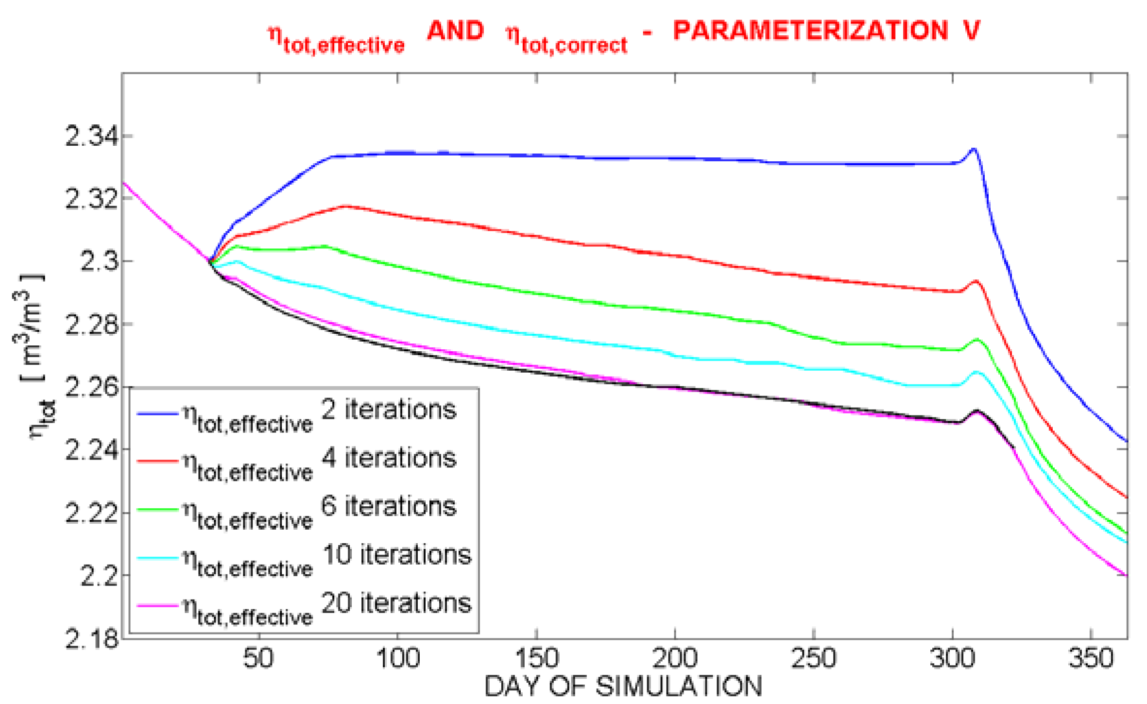
This last correction is inserted in a cycle of 30 iterations per time step. For every iteration the variable
ηtot,effective is recalculated from the
ηw,new values in the previous iteration based on the following scheme:
This cycle was introduced to ensure the convergence of
ηtot,effective, as shown in
Figure 13.
Figure 13.
Trends of ηtot;correct for parameterization V without correction (black line) and of ηtot;effective with corrections (other lines) and with different iterations numbers.
Figure 13.
Trends of ηtot;correct for parameterization V without correction (black line) and of ηtot;effective with corrections (other lines) and with different iterations numbers.
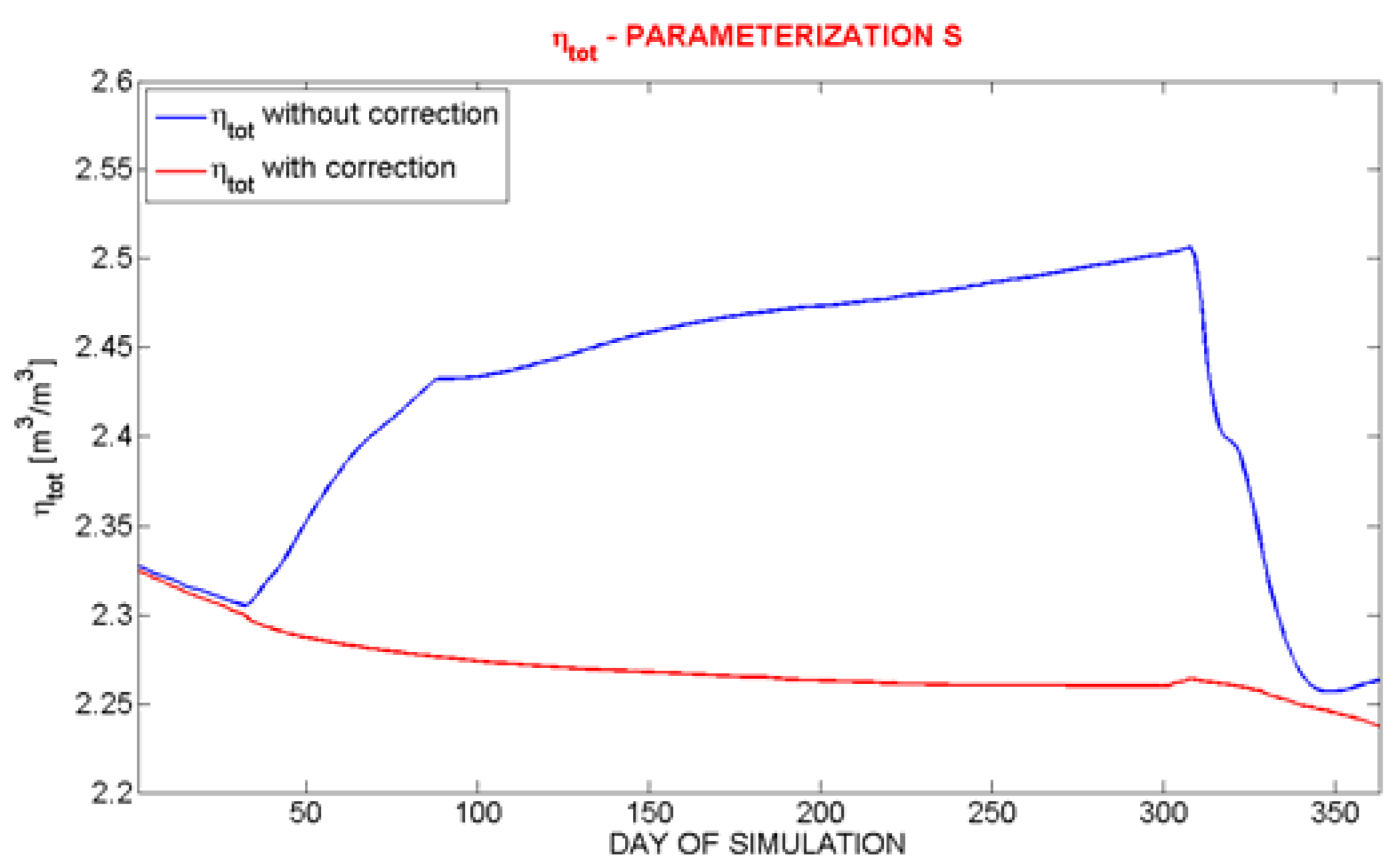
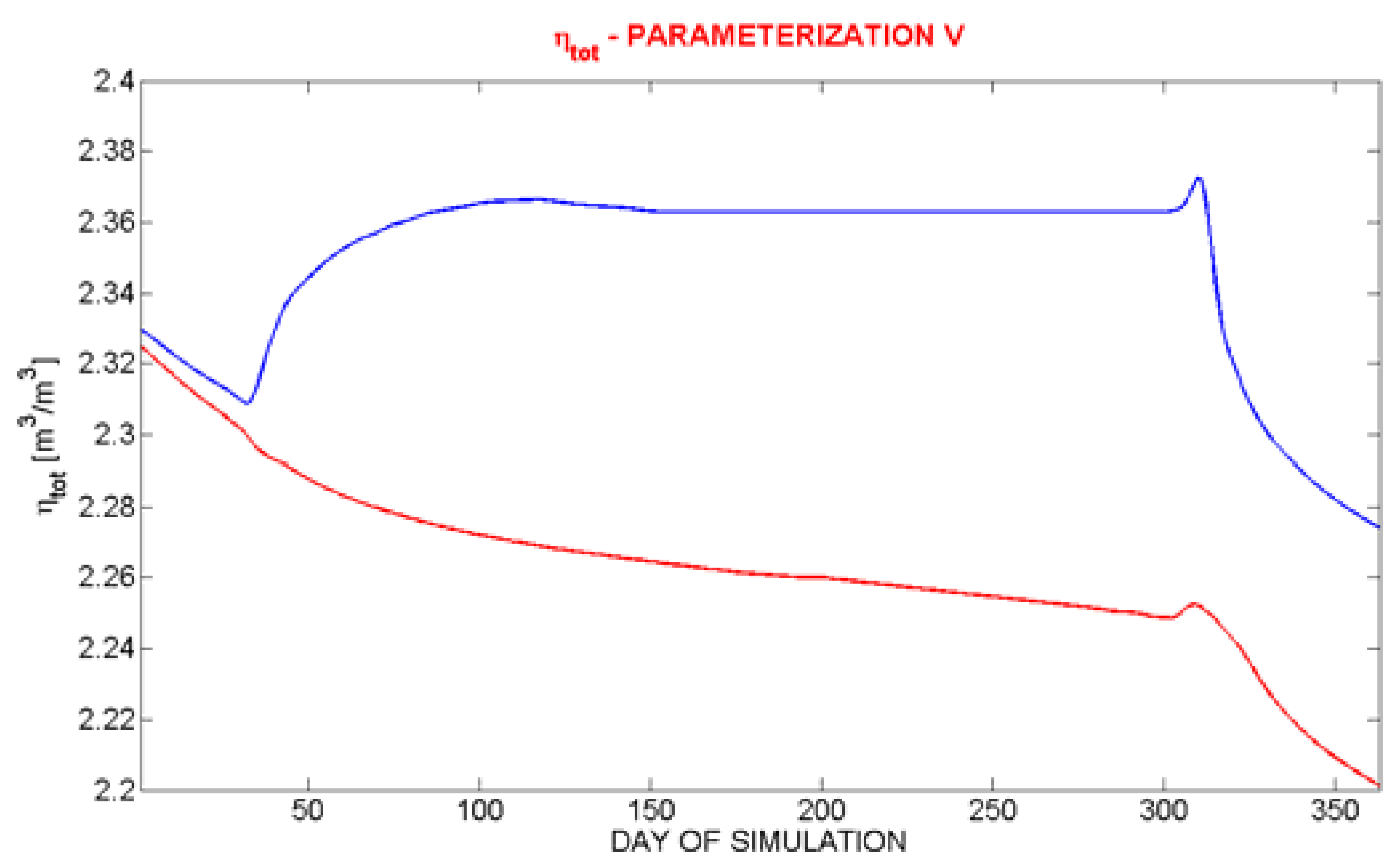
Figure 14,
Figure 15 and
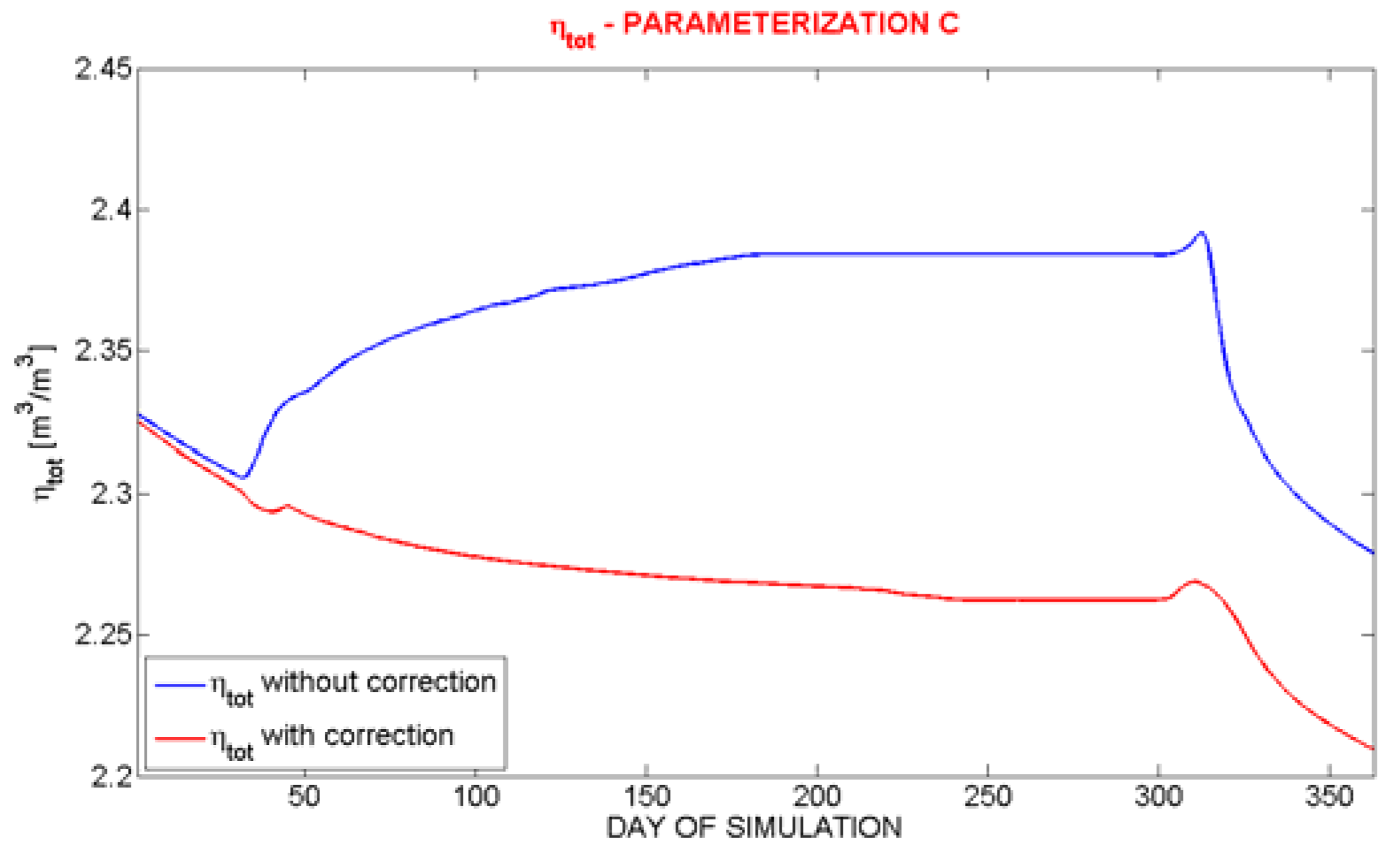
Figure 16 show the total volumetric water content for all soil layers, without (blue line) and with (red line) the above-mentioned correction. In the second case, the trend of
ηtot is justified on the basis of consideration related to hydrological soil balance. The decrease of
ηtot is mainly due to drainage from the bottom layer. In fact, in the period with temperature below zero degrees, the transpiration is stopped and evaporation is reduced.
Figure 14.
Trends of ηtot;correct for simulations without correction (blue line) and of ηtot;effective with correction (red line). In these simulations each soil layer has been initialized with a value of ηw = 0.4 m3/m3.
Figure 14.
Trends of ηtot;correct for simulations without correction (blue line) and of ηtot;effective with correction (red line). In these simulations each soil layer has been initialized with a value of ηw = 0.4 m3/m3.
Figure 15.
Same as
Figure 14 but for the parameterization V.
Figure 15.
Same as
Figure 14 but for the parameterization V.
Figure 16.
Same as
Figure 14 but for the parameterization C.
Figure 16.
Same as
Figure 14 but for the parameterization C.
Another diagnostic to analyze the water overproduction problem is to look at the hydrological balance given by:
In the previous formula
, where i and i-1 are the current and the previous timesteps, respectively, Δt is the model timestep, I is the precipitation, E the evapotranspiration, R the sum of intermediate and surface runoff and D is the drainage from the bottom soil layer.
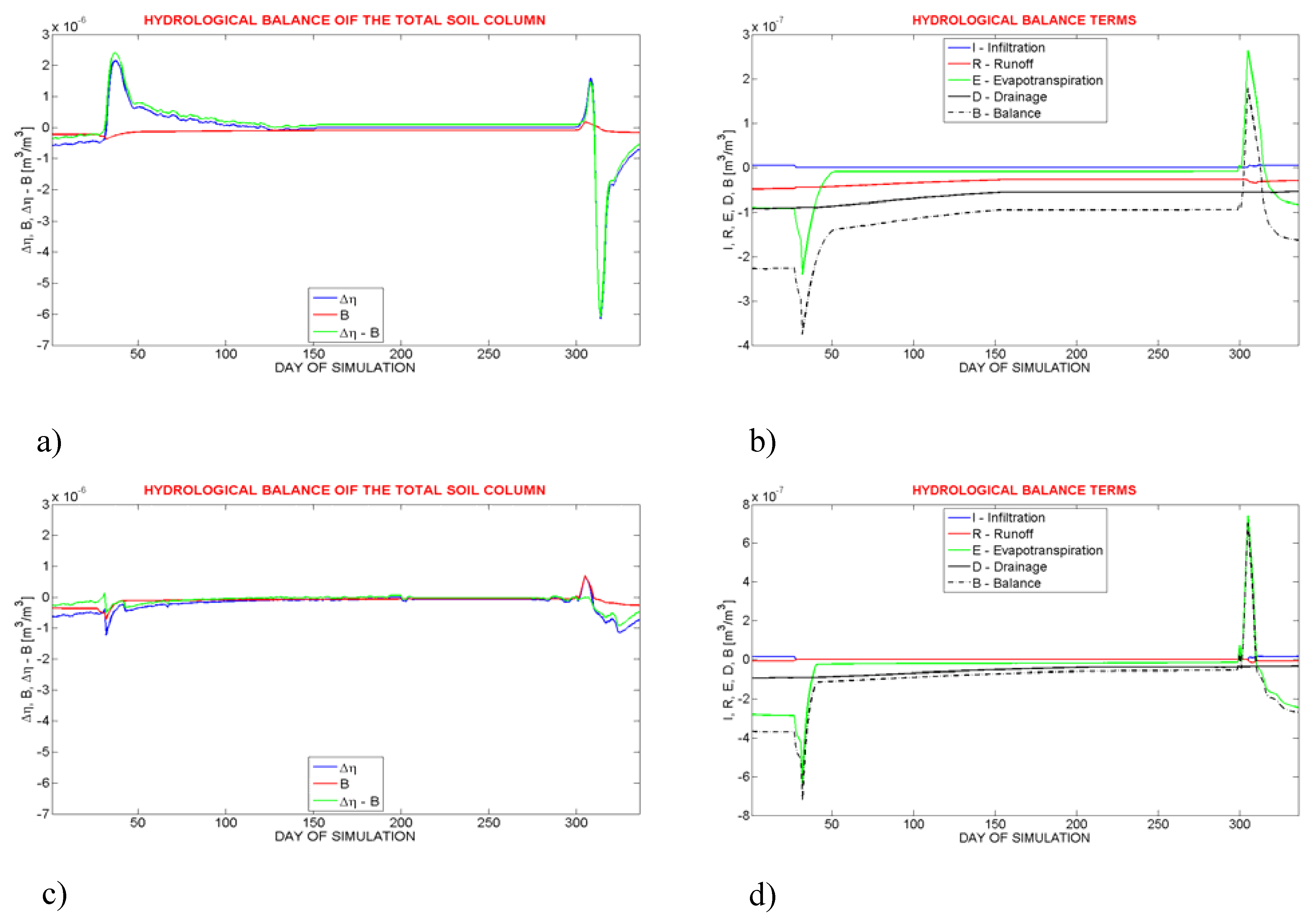
Figure 17 shows the hydrological balance and its components for simulation with and without the correction of the water overproduction correction for the parameterization V. Without the correction there is an unbalance of the hydrological balance during the transition phases (freezing and thawing). Implementing the correction in UTOPIA model, the hydrological balance and hence the mass conservation are respected.
Figure 17.
Hydrological balance and its components with (a, b) and without (c, d) the correction for the water overproduction and relative to the parameterization V. Notice the different scales of the plots (10-6 for the hydrological balance, 10-7 for the components).
Figure 17.
Hydrological balance and its components with (a, b) and without (c, d) the correction for the water overproduction and relative to the parameterization V. Notice the different scales of the plots (10-6 for the hydrological balance, 10-7 for the components).


