1. Introduction
In recent decades, groundwater has been extensively used for drinking, agricultural, and industrial purposes; consequently, its depletion has become a serious problem in many areas worldwide, such as the North China Plain [
1] and the High Plains of the United States [
2]. Because the mean residence time of groundwater reservoir is typically long (~1,400 years [
3]), groundwater is highly vulnerable to excess use and contamination; in the case of groundwater depletion or contamination, aquifers require a long time for recovery and purification.
Therefore, an understanding of groundwater flow systems and groundwater residence time is an important component of the sustainable management of water resources. The use of environmental tracers (see
Figure 1) is one of the most effective approaches in visualizing the movement of groundwater (e.g., [
4,
5]). Tritium (
3H) has been commonly used in hydrologic studies during the last several decades. However, due to its short half-life (12.32 years [
6]), tritium concentration has largely returned to the pre-bomb (natural) background level.
Bomb-produced
36Cl is an alternative to tritium [
7,
8], as it is a long-lived radioisotope of chlorine with a half-life of 3.01 ×10
5 years, decaying to
36Ar by β emission (98.10%) and to
36S by electron capture (1.90%) [
9]. Natural
36Cl in the hydrologic cycle originates mainly from cosmic ray spallation of
40Ar in the stratosphere. The global mean production rate of
36Cl in the atmosphere is estimated to be 21.4 atoms m
−2 s
−1 [
10], which is much lower than that of lighter long-lived radionuclides produced from nitrogen and oxygen (e.g.,
10Be and
14C).
After production,
36Cl leaves the stratosphere and enters the troposphere within about two years [
11]. The
36Cl produced in the atmosphere is mixed with marine-derived stable chlorine (from sea spray), and falls rapidly as wet or dry deposition onto the earth’s surface. The mean residence time in the troposphere is expected to be in the order of weeks, according to estimates of residence times for atmospheric aerosols [
12,
13,
14].
In addition to natural production, significant amounts of
36Cl were produced by thermonuclear testing on small islands or barges (mainly at Bikini and Eniwetok atolls in 1954, 1956, and 1958 [
15]). Neutrons released from the testing activated
35Cl in seawater. Some of this bomb-produced
36Cl reached the stratosphere and spread over the globe. The fallout of bomb-produced
36Cl preserved in ice cores (e.g., [
11]) shows a peak in the late 1950s. Due to the relatively low abundance of
35Cl in the atmosphere, atmospheric tests have a negligible contribution to the production of
36Cl, resulting in the time lag between the
3H and
36Cl peaks (~7 years; see
Figure 1)
Chlorine has a high electron affinity and exists predominantly as the chloride anion (Cl
−) in the environment [
16]. It generally does not participate in redox reactions and biochemical processes, and is not absorbed onto mineral surfaces except under conditions of low pH [
17,
18]. Hence, it moves with water in the natural hydrological cycle without significant chemical interaction. Its simple geochemistry and conservative behavior make chloride an ideal tracer in hydrology [
19]. In addition, it is straightforward to collect samples for analyses of chloride and chlorine isotopes.
The advantage of bomb-produced
36Cl as a hydrological tracer is derived from the fact that the peak is well defined, and that the long half-life of
36Cl makes decay attenuation negligible on the time scale of several decades to centuries (e.g., [
20,
21]). In previous studies, the
36Cl bomb pulse has been used to trace water movement in the unsaturated zone, especially in arid and semi-arid regions (e.g., [
22,
23,
24]); however, few studies have applied this method to tracing young groundwater [
25,
26]. In combination with
3H, bomb-produced
36Cl has been used to estimate the rate of groundwater recharge in a fractured rock aquifer [
25] and to deduce the flow velocity and dispersivity in a sandy aquifer [
26].
The aim of the present study is to investigate the potential of 36Cl in tracing a regional groundwater flow system with a time scale of ~50 years. This paper reports on the observed 36Cl distribution in groundwater beneath an upland–lowland topographic system, and compares the results with existing tritium data. The distribution of 36Cl observed in the present study has implications for the tracer properties of 36Cl, including the bomb-derived component.
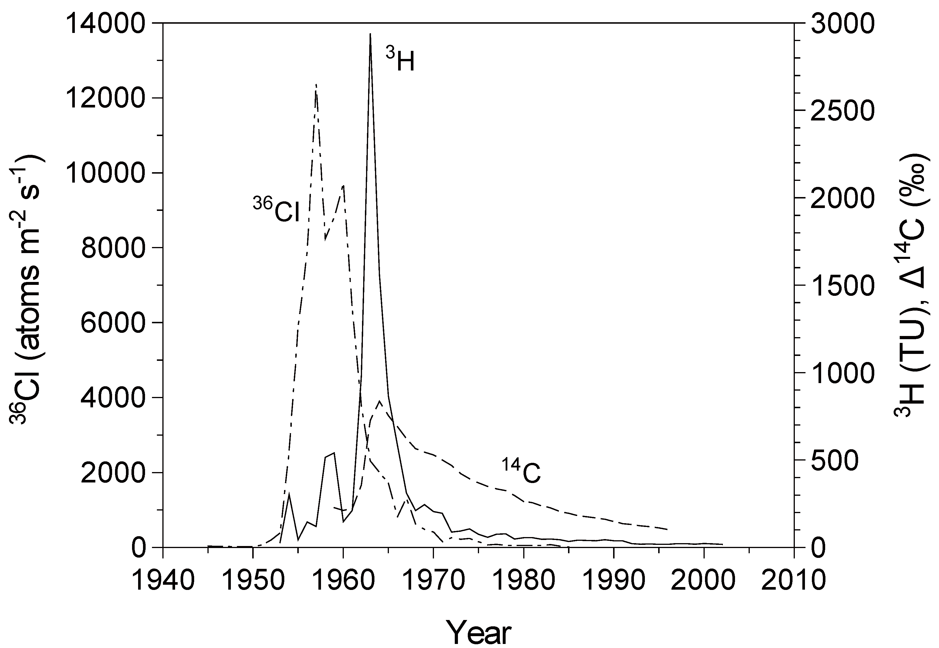
Figure 1.
Atmospheric concentrations or fallout rates of bomb-derived environmental tracers (after [
27]):
36Cl fallout rates at the Dye-3 site, Greenland [
11];
3H concentration in precipitation at Ottawa, Canada [
28]; and atmospheric δ
14C record at Vermunt, Austria (1959–1983); and Schauinsland, Germany (1984–1996) [
29].
2. Study Site and Methods
2.1. Topography, Geology, and Climate
The study area is located in the lower part of the Yoro River basin, northern Boso Peninsula, Central Japan (
Figure 2). The Yoro River runs northward through the central part of the area into Tokyo Bay. The area is characterized by fluvial terraces and alluvial lowlands along the river, and surrounding Pleistocene uplands and hills. The uplands and hills are part of the Shimosa Upland and Kazusa Hills, respectively. The upland surface slopes northwestward, at elevations ranging from ~100 m in the south to ~40 m along Tokyo Bay in the north.
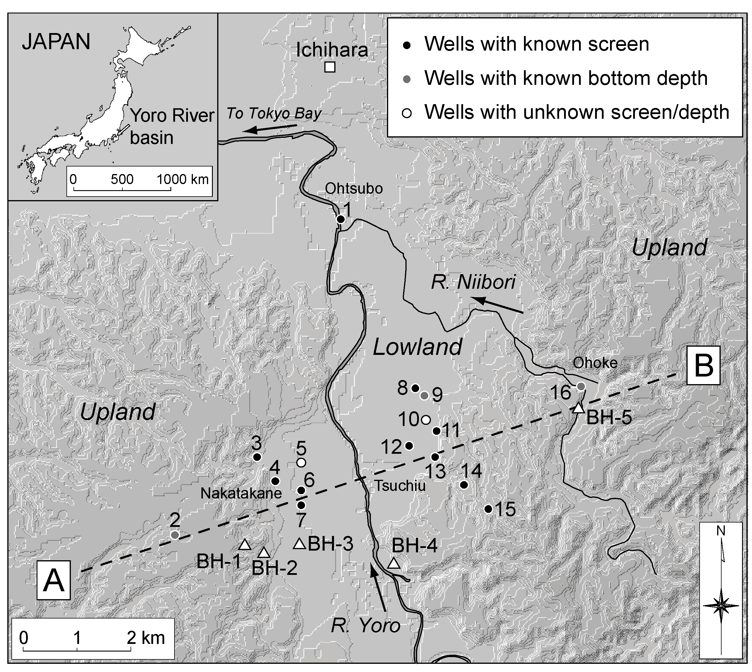
Figure 2.
Locations of sampled irrigation wells in the Yoro River basin. Open triangles indicate selected borehole locations from Kondoh (1985) [
30] and Chiba Prefectural Research Institute for Environmental Pollution (1974) [
31].
Figure 2.
Locations of sampled irrigation wells in the Yoro River basin. Open triangles indicate selected borehole locations from Kondoh (1985) [
30] and Chiba Prefectural Research Institute for Environmental Pollution (1974) [
31].
The following geological summary of the study area is based on Tokuhashi and Endo (1984) [
32]. The area is dominated by (in ascending stratigraphic order) middle Pleistocene upper Kazusa Group sediments, middle–upper Pleistocene Shimosa Group sediments, upper Pleistocene terrace deposits with Kanto Loam, Holocene terrace deposits, and alluvial deposits. The Kazusa and Shimosa groups strike northeast–southwest, dipping gently northwest at 0.4–6.0°. The alluvium is distributed mainly in the lowlands along the Yoro River, with lesser amounts in dissected valleys in the hills and uplands.
The Kazusa Group occurs extensively throughout the Kazusa Hills in the middle to northern part of the Boso Peninsula. Of the 12 formations in this group, only the upper formations (i.e., the Kokumoto, Kakinokidai, Chonan, Kasamori, and Kongochi formations, in ascending stratigraphic order) are exposed in the study area. The Kazusa Group is composed mainly of alternating deep-water sand and mudstone, with lesser shallow-water sandy mudstone, sand, and cross-bedded gravelly sands.
The Shimosa Group, which overlies the Kazusa Group, is widely exposed in the Shimosa Uplands, in the northern part of Boso Peninsula. This group consists of seven formations (i.e., the Jizodo, Yabu, Kamiizumi, Kiyokawa, Yokota, Kioroshi, and Anesaki formations, in ascending stratigraphic order), with a maximum total thickness of over 250 m. The uppermost Anesaki Formation consists of fresh‑water sediments. Other formations in the group are characterized by sedimentary cycles that start from fresh- or brackish-water muds and end with shallow-marine sands.
The study area is located in a humid temperate climate, with an annual mean temperature of ~15 °C and average annual precipitation ranging from 1,294 mm at Chiba on the northwestern side of the study area, near the coast along Tokyo Bay, to 1,590 mm at Ushiku in the southern hilly area (average values for 1971–2000 [
33]). The estimated annual evapotranspiration rate is ~700 mm at Chiba [
30].
2.2. Hydrogeology
In this area, the Kasamori Formation, which is dominated by muddy sandstone, probably acts as the hydraulic basement for the groundwater in the overlying Shimosa Group sediments. Mainly in the upland regions, groundwater is used extensively for irrigation and drinking water. The main aquifers supplying the groundwater located within the Jizodo and Yabu formations, which is composed by alternating sand and mud [
30] (
Figure 3). The depth to the water table is generally small, e.g., 3–5 m at Nakatakane area (near wells 3, 4, and 7), ~3 m at Ohtsubo area (near well 1), and ~3 m at Ohoke area (near well 16) [
31] (see
Figure 2 for the locations). Thus, the shape of the water table is expected to reflect the surface topography. Aquifer tests showed relatively high hydraulic conductivities (10
−3–10
−2 cm/s) in this area [
30].
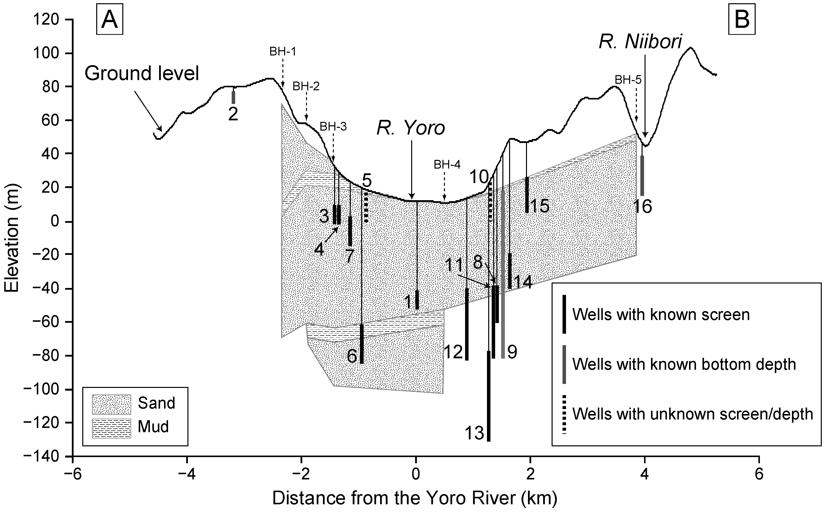
Figure 3.
Cross-section showing the geology and the distribution of well screens projected onto the line A–B in
Figure 2. The screen intervals or bottom depths of the wells are given in
Table 1. Geological data is from Kondoh (1985) [
30] and Chiba Prefectural Research Institute for Environmental Pollution (1974) [
31] (see
Figure 2 for the borehole locations).
Kondoh (1985) [
30] performed a three-dimensional numerical simulation of regional groundwater flow in this area. The results revealed the importance of topographic controls on the groundwater flow, as well as the minor contribution of the northwestward dip of the geological structure. These findings were confirmed by the distribution of tritium concentrations in groundwater within the basin [
30]: High tritium concentrations occur in the upland region, and low concentrations in the lowland region, along the Yoro River (
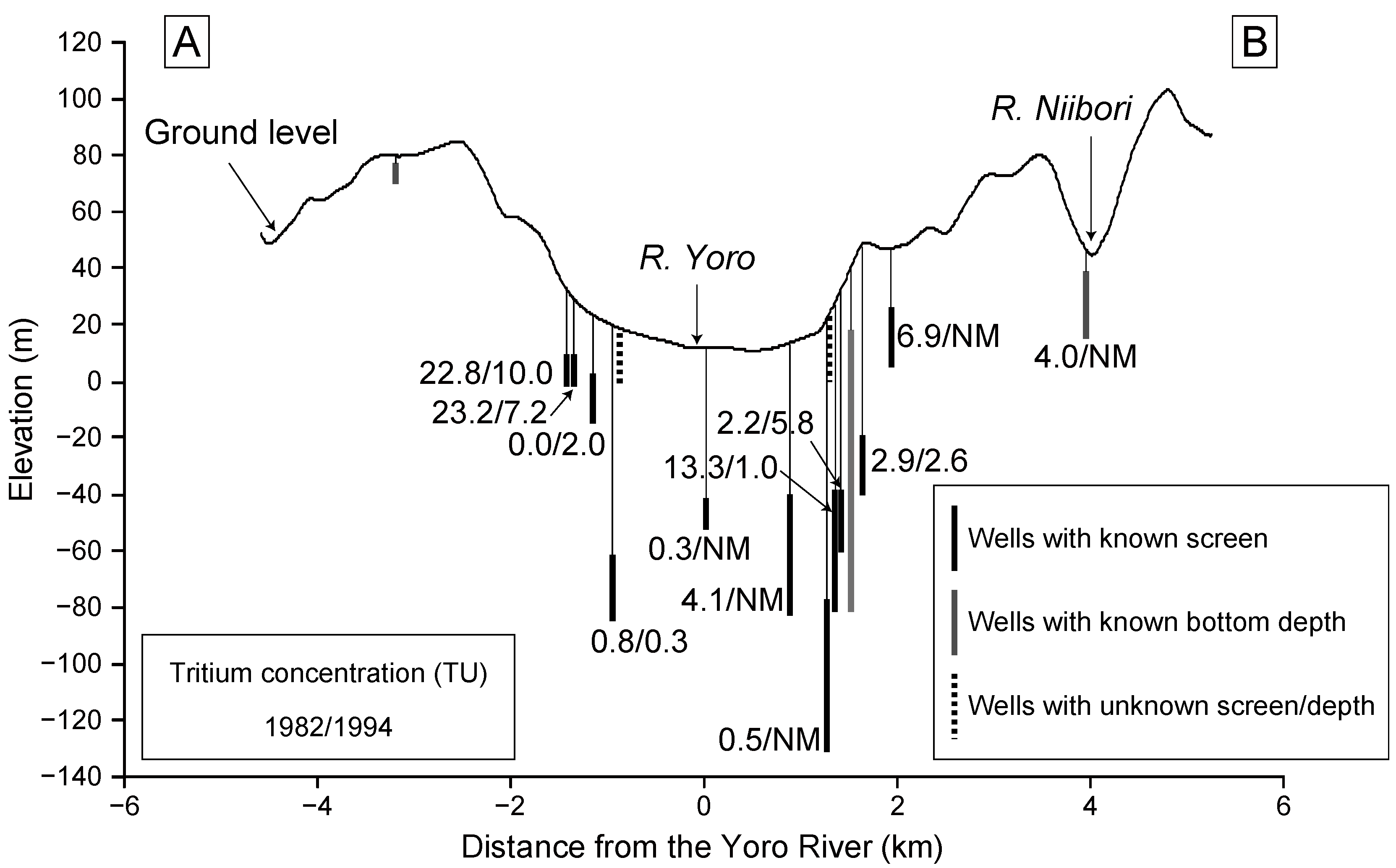
Figure 4). This distribution indicates the occurrence of relatively young groundwater ages in the upland region, and older ages in the lowland area. It also shows that recharge occurs mainly in upland areas and that groundwater essentially flows into the lowland area, eventually discharging into the Yoro River. Because groundwater samples in the lowland area showed very low tritium concentrations at that time (1982), the regional groundwater flow system from the upland to lowland region appears to have a residence time greater than 30 years (recharged before 1953; see
Figure 1).
In 1994, Miyazawa (1995) [
34] revisited the regional groundwater flow system in the Yoro River basin by measuring tritium concentrations in groundwater samples obtained from some of the locations sampled previously by Kondoh (1985) [
30]. Even though 12 years had passed since the first study, groundwater in the lowland area still contained low tritium concentrations (
Figure 4). This observation clearly indicates the presence of pre-bomb groundwater recharged before 1953 (age > 40 years).
Figure 4.
Tritium concentrations measured in 1982 [
30] and 1994 [
34]. Left and right values for each well are tritium data measured in 1982 and 1994, respectively. Wells without values indicate that tritium data are unavailable. NM: not measured.
Figure 4.
Tritium concentrations measured in 1982 [
30] and 1994 [
34]. Left and right values for each well are tritium data measured in 1982 and 1994, respectively. Wells without values indicate that tritium data are unavailable. NM: not measured.
2.3. Methodology
Sites for groundwater sampling for
36Cl measurements were mainly irrigation wells for which tritium data are available [
30,
34]. Sampling was performed during the irrigation period for paddy fields in the summer of 2004 (24 July and 13 August). Sixteen groundwater samples were collected from pumped irrigation wells located within the basin, ranging from lowland to upland areas (
Figure 2).
The samples were analyzed for dissolved inorganic ions, silica, stable isotopes of oxygen and hydrogen, and 36Cl, at the University of Tsukuba, Japan. Prior to chemical analyses, the samples were passed through 0.20 μm filters (25HP020AN, Advantec, Tokyo, Japan). Concentrations of major dissolved cations (Na+, K+, Mg2+, and Ca2+) and silica (SiO2) were measured with an ICP–AES (inductively coupled plasma–atomic emission spectroscopy) system (ICAP-757, Nippon Jarrell-Ash, Kyoto, Japan). Bicarbonate (HCO3−) concentrations were determined by titration with dilute H2SO4 solution. Concentrations of major anions (Cl−, NO3−, and SO42−) were measured by ion chromatography (QIC Analyzer, Dionex, Sunnyvale, CA, U.S.). Stable isotopic ratios of oxygen and hydrogen (δ18O and δD) were determined with a mass spectrometer (MAT252, Thermo Finnigan, Bremen, Germany). The analytical errors were 0.1‰ and 1‰ for δ18O and δD, respectively.
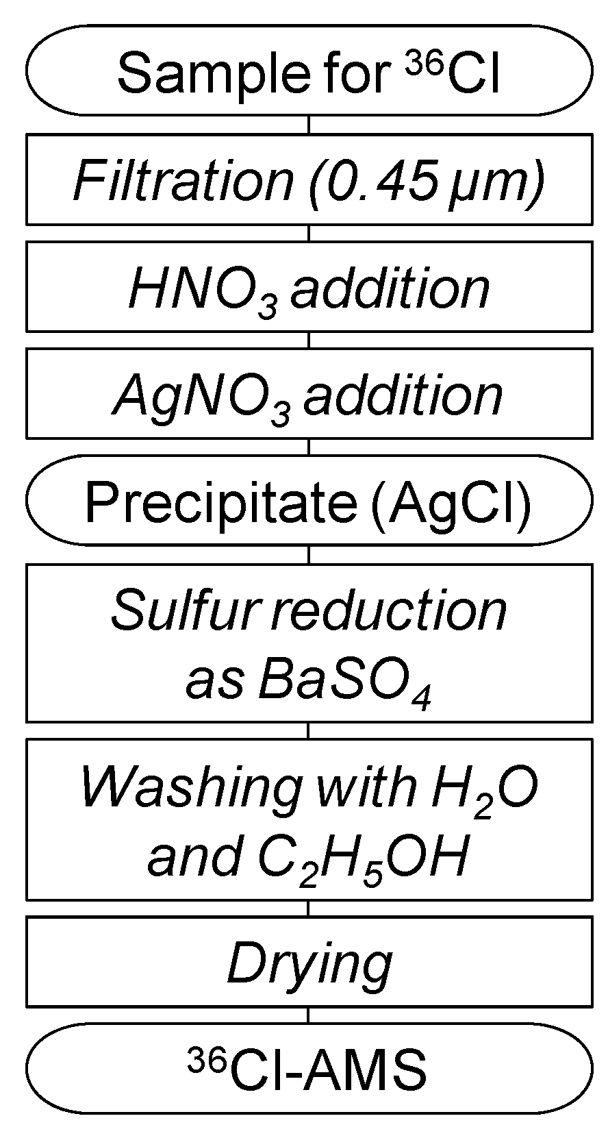
Figure 5 summarizes the preparation procedure used in this study. All samples for measurements of
36Cl by AMS (
36Cl-AMS) were passed through 0.45 μm filters (JHWP04700, Millipore). The samples were then processed according to the preparation scheme shown in
Figure 5. Water samples containing ~1 mg of Cl were acidified with 1 mL of 13 M of HNO
3. Chloride was then precipitated as silver chloride (AgCl) by adding excess AgNO
3, and was separated by centrifugation. The AgCl precipitate was dissolved once in 3 M of NH
4OH, and saturated Ba(NO
3)
2 solution was added to the solution. The solution was allowed to stand overnight in an oven at ~60 °C, to effectively precipitate SO
42− as BaSO
4. This precipitate was removed by filtration with a 0.20 μm membrane filter (25HP020AN, Advantec), and the filtrate was acidified by the addition of 13 M of HNO
3 to precipitate AgCl again.
Figure 5.
Summary of the sample preparation scheme for 36Cl-AMS.
Figure 5.
Summary of the sample preparation scheme for 36Cl-AMS.
Because the isobar
36S (natural abundance, 0.02% [
9]) strongly interferes with
36Cl measurements by accelerator mass spectrometry (AMS), the chemical reduction of sulfur is of major importance in preparing AgCl samples. The removal of sulfur (in the form of SO
42−) can be achieved by the precipitation of BaSO
4 (e.g., [
35]), by differential elution from an anion exchange resin [
36], or by absorption onto a cation exchange resin (in the form of BaSO
4) [
37]. The main part of sample preparation, including sulfur reduction, was performed in an air-conditioned room to prevent additional sulfur contamination and was performed under dark conditions to avoid the photolytic decomposition of AgCl.
The sample was purified by repeated precipitation of AgCl with HNO3 and dissolution in NH4OH. To further exclude remaining impurities, the AgCl precipitate was washed with Milli-Q ultrapure water twice and with 99.5% C2H5OH twice using ultrasonic vibration. The overall chemical yield of chlorine was typically about 80%. For subsequent 36Cl-AMS, a benzene solution saturated with fullerene (C60) was added to each sample (~20 μL per 1 mg of AgCl) and the sample was dried in an oven at 120 °C for more than 24 hours. Finally, the sample was pressed into the target holder for 36Cl-AMS.
36Cl/Cl ratios were measured using the AMS system at the Tandem Accelerator Complex, Research Facility Center for Science and Technology, University of Tsukuba [
38], along with diluted NIST
36Cl standards (
36Cl/Cl = 1.60 ×10
−12 [
39]). The electric current of
35Cl
− was measured by a Faraday cup located immediately after the ion source, whereas
36Cl ions were counted at the final detector, being distinguished from
36S. The
36Cl/
35Cl
− ratio (counts/μC) derived from the measurements was normalized to that obtained for the standard sample. The obtained
36Cl/Cl ratio of the sample was subjected to a background correction using the measured ratio of a chemical blank prepared from a sample of Himalayan halite. The overall precision of the system was better than 2%, and the background level of
36Cl/Cl was ~1 ×10
−15 [
38]. The calculated
36Cl/Cl ratio of the sample includes the statistical error derived from the uncertainties (1σ) calculated for the sample, the standard, and the blank.
3. Results and Discussions
Table 1 lists the stable isotopic compositions and
36Cl data for the analyzed samples, along with existing data for tritium [
30,
34]. Major dissolved ions and SiO
2 concentrations are given in
Table 2. Samples 2, 3, 7, and 16, show much higher Cl
− concentrations than the other samples (
Table 2). Samples 2 and 16, which were taken from shallow wells (<30 m;
Table 1) located far from the Yoro River, have high NO
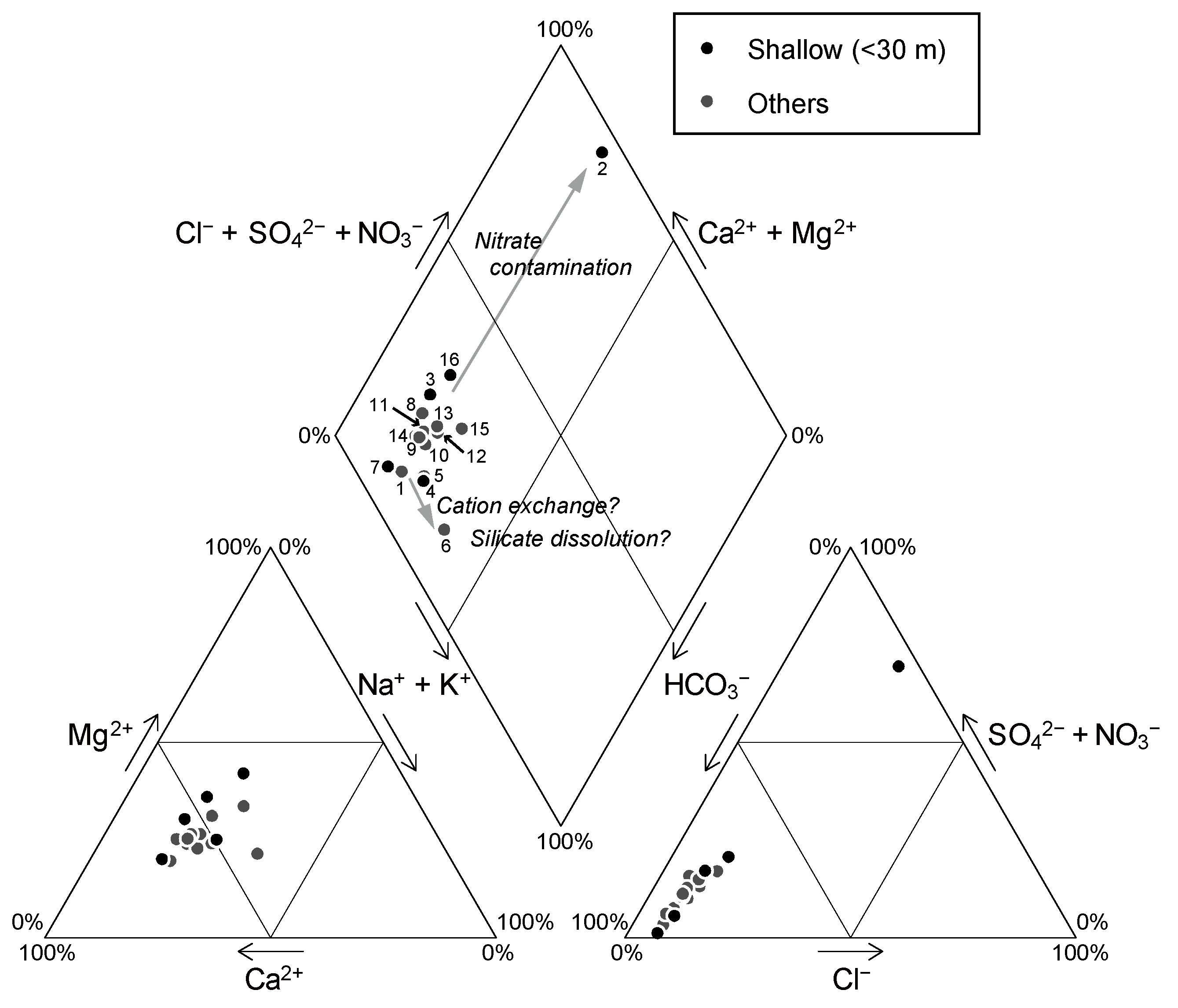
3− concentrations (>30 mg/L), indicating the influence of agricultural fertilizers. This trend of nitrate contamination is confirmed by a Piper diagram (
Figure 6). These two samples (Samples 2 and 16) may contain anthropogenic chloride derived from fertilizer, which would lower their original
36Cl/Cl values to some extent; consequently, these samples were excluded from the discussion on the distribution of
36Cl/Cl values. Although the
36Cl/Cl values obtained for Sample 2 are not considered in the interpretations presented below, the low SiO
2 concentration obtained for this sample (
Table 2) suggests a young groundwater age.
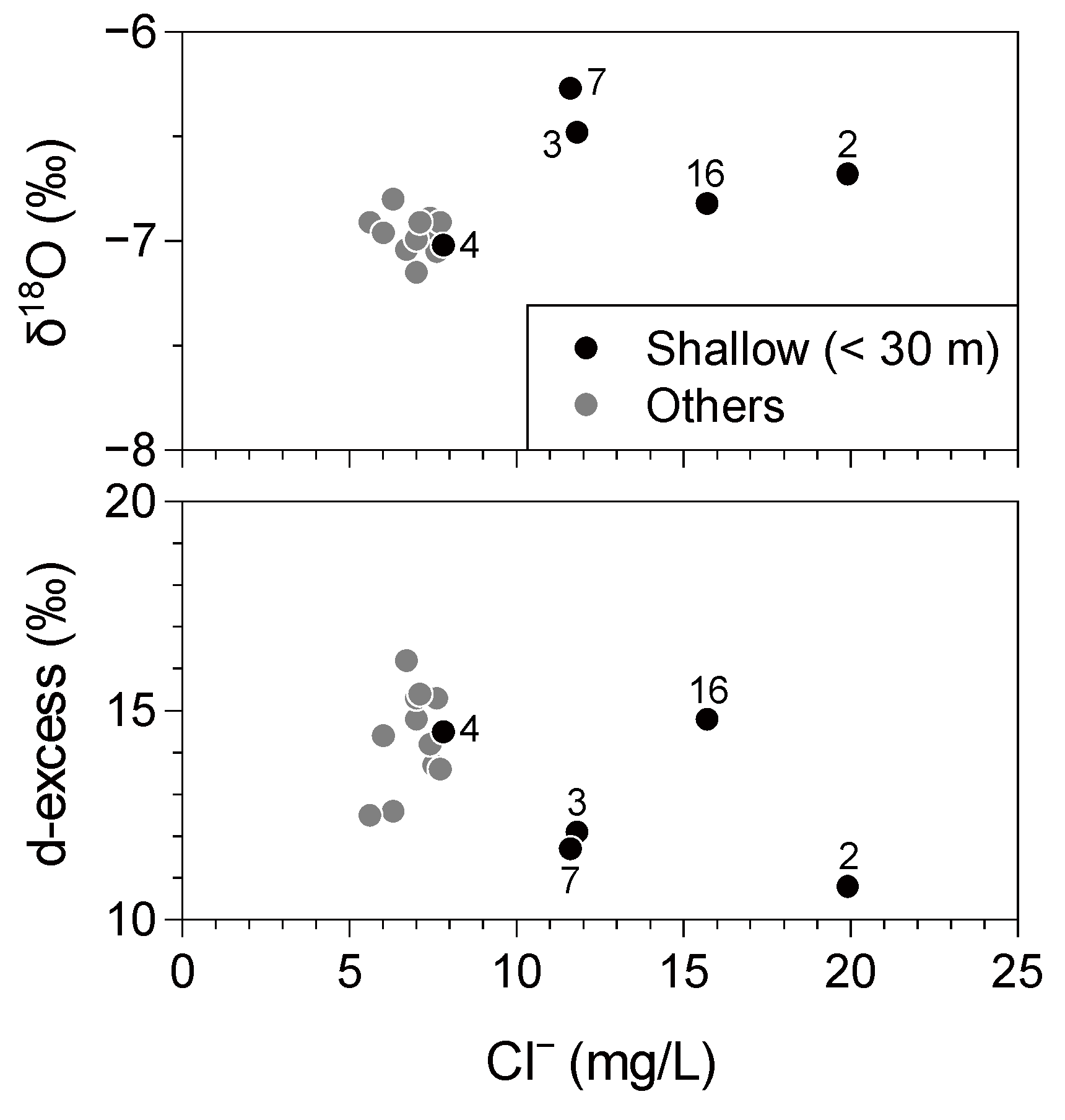
The stable isotopic compositions showed a relatively small variation mostly in the range of −7.1‰ to −6.8‰ and −43‰ to −40‰ for δ
18O and δD, respectively, although the bottom depth (or screen depth) of the wells varies from ~10 m to ~100 m. This range of variation is almost consistent with the results of a δ
18O–δD mapping study of surface waters and shallow groundwaters in Japan [
40]. The small variation may indicate that the investigated aquifers of the study area are recharged at almost similar elevation, probably in upland areas. Shallow wells tend to show slightly higher stable isotopic ratios, while deeper wells have lower δ
18O and δD values (
Table 1;
Figure 6). This may suggest an influence of a local recharge from the surface, which can possess higher δ
18O and δD values. Among the samples with high Cl
− concentrations, Samples 2, 3, and 7 show relatively low d-excess values (
Table 1;
Figure 6), as defined by d = 8δ
18O − δD, that may indicate the influence of evaporation. Because evaporation does not affect
36Cl/Cl values, Samples 3 and 7 are considered in the following discussion.
Figure 6.
δ18O and d-excess values for groundwater plotted against the Cl− concentrations.
Figure 6.
δ18O and d-excess values for groundwater plotted against the Cl− concentrations.
Table 1.
36Cl and isotopic data for groundwater samples from the Yoro River basin.
Table 1.
36Cl and isotopic data for groundwater samples from the Yoro River basin.
| Sample | Depth | 36Cl/Cl | 36Cl | 3Ha | 3Hb | δ18O | δD | d-excess |
|---|
| No. | (m) | (10−15) | (106 atoms/L) | (TU) | (TU) | (‰) | (‰) | (‰) |
|---|
| 1 | 48–60 | 25 ± 3 | 2.7 ± 0.3 | 0.3 ± 0.3 | NM | −6.8 | −42 | 12.6 |
| 2 | 10 | 61 ± 5 | 20.6 ± 1.8 | NM | NM | −6.7 | −43 | 10.8 |
| 3 | 14–27 | 140 ± 9 | 27.9 ± 1.8 | 22.8 ± 0.5 | 10.0 ± 1.3 | −6.5 | −40 | 12.1 |
| 4 | 24–27 | 150 ± 9 | 19.9 ± 1.2 | 23.2 ± 0.5 | 7.2 ± 1.2 | −7.0 | −42 | 14.5 |
| 5 | NK | 29 ± 20 | 2.8 ± 1.9 | NM | NM | −6.9 | −43 | 12.5 |
| 6 | 80–105 | 17 ± 3 | 1.8 ± 0.3 | 0.8 ± 0.3 | 0.3 ± 0.5 | −7.0 | −41 | 14.4 |
| 7 | 18–32 | 117 ± 10 | 23.1 ± 2.0 | 0.0 ± 0.4 | 2.0 ± 1.1 | −6.3 | −38 | 11.7 |
| 8 | 54–78 | 258 ± 11 | 33.2 ± 1.5 | 5.8 ± 0.8 | 5.8 ± 0.8 | −7.1 | −41 | 15.3 |
| 9 | 100 | 161 ± 14 | 21.2 ± 1.9 | NM | NM | −6.9 | −42 | 13.6 |
| 10 | NK | 65 ± 13 | 7.8 ± 1.6 | NM | NM | −7.0 | −41 | 14.8 |
| 11 | 56–100 | 128 ± 8 | 15.4 ± 1.0 | 13.3 ± 0.5 | 1.0 ± 0.6 | −6.9 | −40 | 15.4 |
| 12 | 56–100 | 216 ± 13 | 27.5 ± 1.7 | 4.1 ± 0.3 | NM | −6.9 | −42 | 13.7 |
| 13 | 95–150 | 362 ± 20 | 43.2 ± 2.4 | 0.5 ± 0.5 | 5.5 ± 1.0 | −7.1 | −42 | 15.3 |
| 14 | 50–72 | 225 ± 15 | 28.2 ± 1.9 | 2.9 ± 0.6 | 2.6 ± 0.9 | −6.9 | −41 | 14.2 |
| 15 | 32–54 | 345 ± 17 | 39.4 ± 2.0 | 6.9 ± 0.6 | NM | −7.0 | −40 | 16.2 |
| 16 | 25 | 243 ± 18 | 65.1 ± 4.8 | 4.0 ± 0.4 | 11.8 ± 1.4 | −6.8 | −40 | 14.8 |
Table 2.
Dissolved major ions and silica concentrations in groundwater from the Yoro River basin.
Table 2.
Dissolved major ions and silica concentrations in groundwater from the Yoro River basin.
| Sample | Na+ | K+ | Mg2+ | Ca2+ | Cl− | NO3− | SO42− | HCO3− | SiO2 |
|---|
| No. | (mg/L) | (mg/L) | (mg/L) | (mg/L) | (mg/L) | (mg/L) | (mg/L) | (mg/L) | (mg/L) |
|---|
| 1 | 7.7 | 7.3 | 7.9 | 30.6 | 6.3 | 0.2 | 4.0 | 143.4 | 45.6 |
| 2 | 8.9 | 5.2 | 11.6 | 15.9 | 19.9 | 93.3 | 0.1 | 6.1 | 18.8 |
| 3 | 9.5 | 7.1 | 9.2 | 48.2 | 11.8 | 0.8 | 29.3 | 163.5 | 55.6 |
| 4 | 10.4 | 10.7 | 8.7 | 28.3 | 7.8 | 0.3 | 7.1 | 142.7 | 43.1 |
| 5 | 9.3 | 8.1 | 7.2 | 25.1 | 5.6 | 0.2 | 8.1 | 118.3 | 55.5 |
| 6 | 19.4 | 7.7 | 7.5 | 24.3 | 6.0 | 0.2 | 8.2 | 151.3 | 57.3 |
| 7 | 10.6 | 5.9 | 14.4 | 42.1 | 11.6 | 0.2 | 2.7 | 280.6 | 47.6 |
| 8 | 9.4 | 7.5 | 11.2 | 42.6 | 7.6 | 0.2 | 25.5 | 160.4 | 57.9 |
| 9 | 9.5 | 7.8 | 10.0 | 36.3 | 7.7 | 0.2 | 16.2 | 150.7 | 62.0 |
| 10 | 8.0 | 6.4 | 7.8 | 25.4 | 7.0 | 0.3 | 10.6 | 111.0 | 60.3 |
| 11 | 8.8 | 7.0 | 9.5 | 32.2 | 7.1 | 2.2 | 15.1 | 133.6 | 63.1 |
| 12 | 7.6 | 7.2 | 6.4 | 25.3 | 7.5 | 0.2 | 13.3 | 100.0 | 54.9 |
| 13 | 8.4 | 5.6 | 9.0 | 22.6 | 7.0 | 0.2 | 15.8 | 103.7 | 60.5 |
| 14 | 8.6 | 7.3 | 7.5 | 39.2 | 7.4 | 0.2 | 14.6 | 145.8 | 52.5 |
| 15 | 7.2 | 6.2 | 7.1 | 13.6 | 6.7 | 3.4 | 10.4 | 68.9 | 65.6 |
| 16 | 11.3 | 7.5 | 16.8 | 35.4 | 15.7 | 32.0 | 10.3 | 143.4 | 61.2 |
Figure 7.
Chemical compositions of groundwater shown in a Piper diagram.
Figure 7.
Chemical compositions of groundwater shown in a Piper diagram.
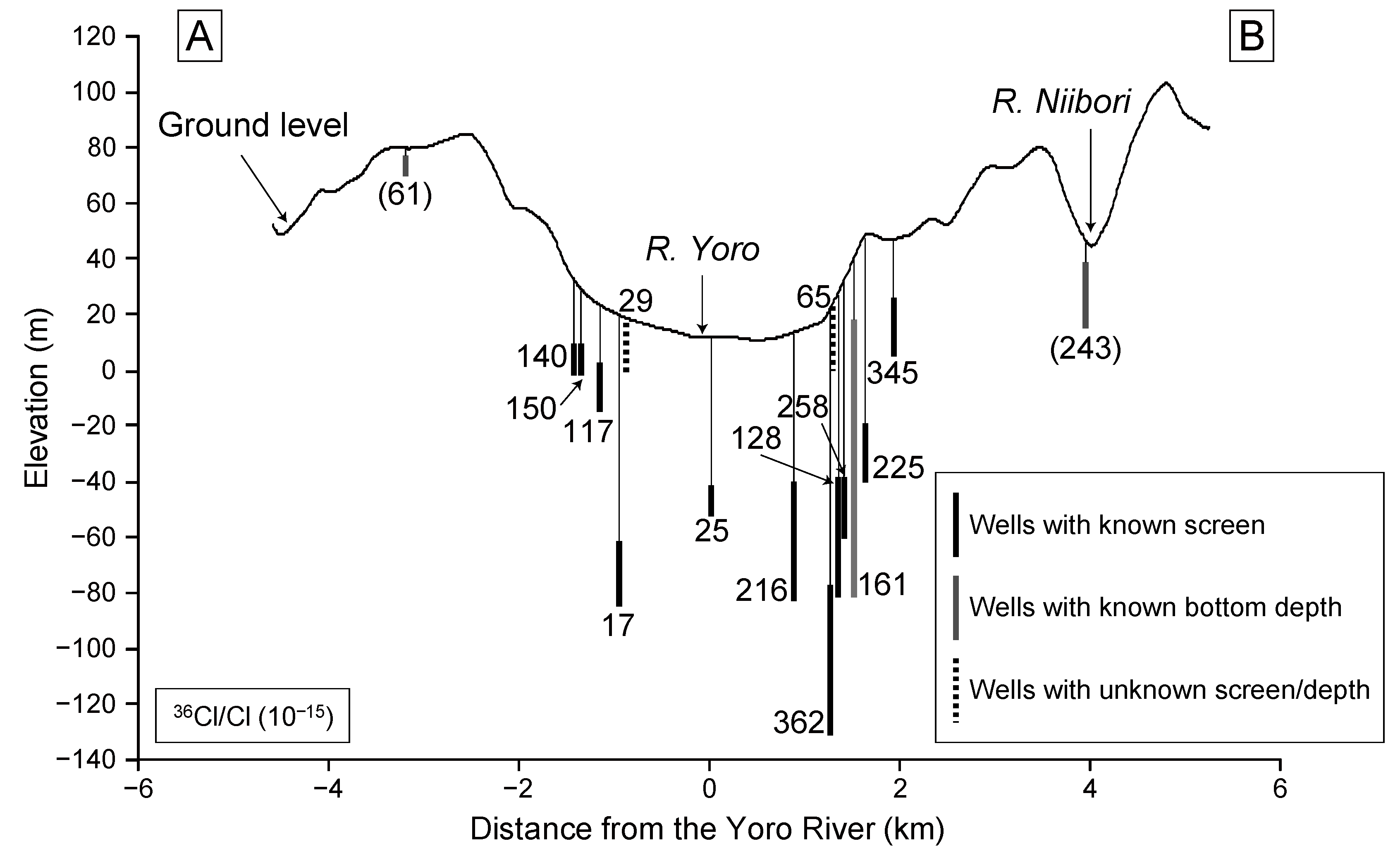
Figure 8 shows the distribution of
36Cl/Cl values projected onto the line A–B in
Figure 2. Although Sample 1 is located relatively far from the projection line, it was also included because it represents groundwater in the discharge area. The overall distribution shows low
36Cl/Cl values in the lowland area along the river, and higher values toward upland areas, except for nitrate-contaminated samples. The observed distribution is basically consistent with the groundwater flow system traced by tritium in 1982 and 1994 (
Figure 4), which showed relatively high concentrations in upland areas and low concentrations in lowland areas. One difference in this regard is that relatively high
36Cl/Cl values are found near the upland area on the eastern side of the Yoro River. This result is expected if we consider the time that has passed since tritium concentrations were measured, as the groundwater could have flowed further toward the lowland area during this time.
Figure 8.
Cross-sectional distribution of 36Cl/Cl values in the Yoro River basin. Parentheses indicate samples with high NO3− concentrations.
Figure 8.
Cross-sectional distribution of 36Cl/Cl values in the Yoro River basin. Parentheses indicate samples with high NO3− concentrations.
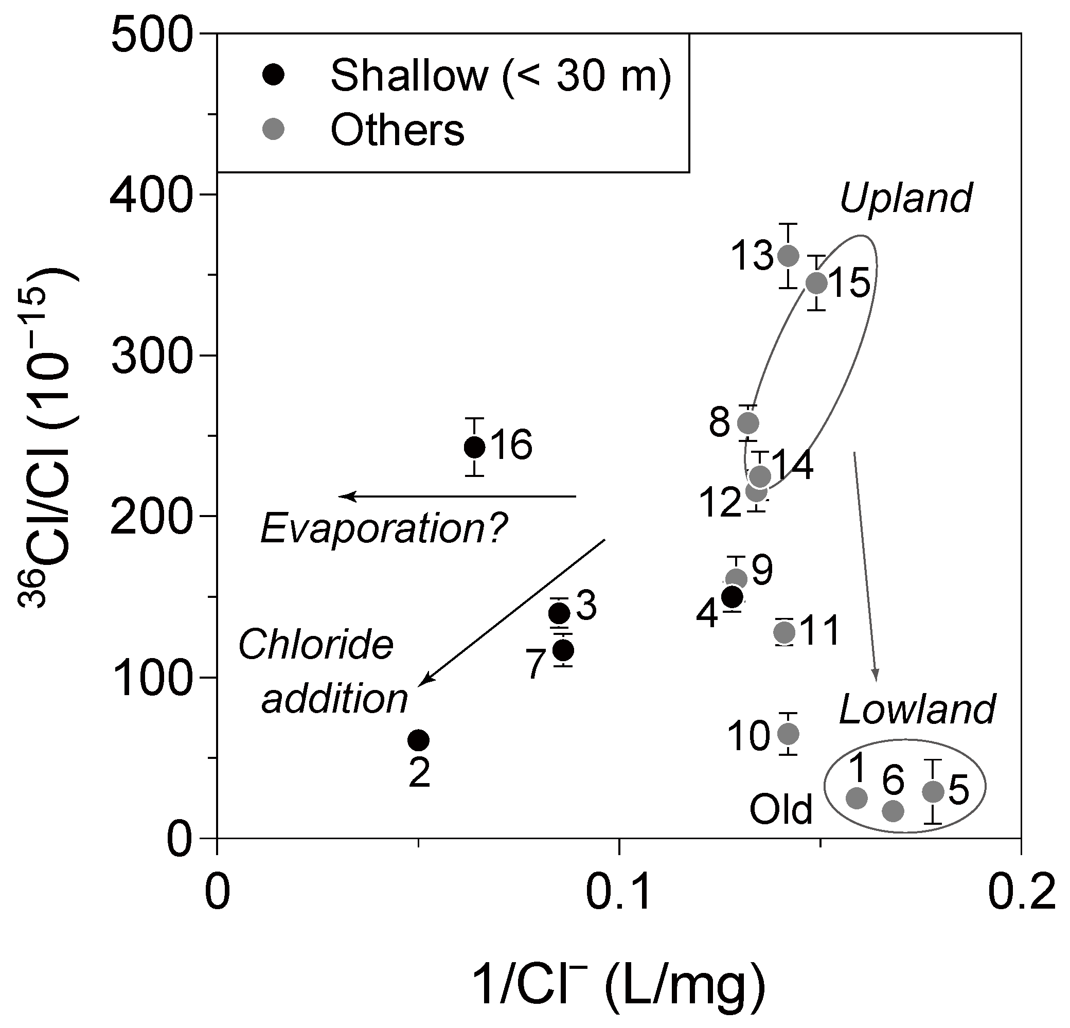
To further examine the nature of hydrological processes operating in the basin,
Figure 9 shows
36Cl/Cl values plotted against the reciprocal of Cl
− concentrations. Samples obtained from shallow wells (<30 m) show higher Cl
− concentrations than do the other samples, which again suggests the influence of non-meteoric chloride and/or evaporation. Among the remaining samples (
i.e., samples from deeper wells, including two samples from unknown depths), two samples from the upland area (Samples 14 and 15) have high
36Cl/Cl values (
Figure 8). The
36Cl/Cl values has a roughly decreasing trend northwestward from well 15 to well 10, except for wells 8 and 9 (
Figure 2 and
Figure 8). Because these wells are located slightly north of the Tsuchiu area (
Figure 2), they are possibly on a different flow line from the other samples. Conversely, three representative samples of the lowland area (Samples 1, 5, and 6), show markedly low
36Cl/Cl values (<30 ×10
−15). This difference demonstrates that pre-bomb (
i.e., ages > 50 years) groundwater remains in the lowland area, suggesting residence times in excess of 50 years for the regional groundwater flow system, which is longer than that estimated previously (up to 40 years) [
30,
34]. Because most of the other samples, except for the lowland samples, show elevated
36Cl/Cl values, their ages are likely to be in the range of 25–50 years (see
Figure 1).
Figure 9.
36Cl/Cl values for groundwater plotted against the reciprocal of Cl− concentrations.
Figure 9.
36Cl/Cl values for groundwater plotted against the reciprocal of Cl− concentrations.
The Na/Cl molar ratios of the three lowland samples (Samples 1, 5, and 6) tend to have higher values (1.9, 2.5, and 5.0, respectively) than those of the other samples (0.7–2.1), as calculated from
Table 2. This result may reflect a cation exchange reaction between Ca
2+ in groundwater and Na
+ in the matrix materials of the aquifer, or silicate dissolution (see
Figure 7). Because the content of TDS (total dissolved solids) in Sample 6 shows no significant increase compared with that in other samples, the high Na/Cl value may have been derived mainly from a cation exchange reaction.
Considering the slightly lower Cl
− concentrations in lowland samples compared with upland samples (
Figure 9), it is possible that human activity (anthropogenic chloride derived from the application of agricultural fertilizer) has had an increasing influence on recharging groundwater (mainly in the upland area). However, this would not lead to a significant contribution on the observed
36Cl/Cl ratios, as indicated by the slight increase in chloride concentrations (~20%). The remarkably high Na/Cl value for Sample 6 suggests it has a relatively old age, which in turn supports the interpretations based on the distribution of
36Cl throughout the basin.


