Comparison of Water Flows in Four European Lagoon Catchments under a Set of Future Climate Scenarios

Hesse, Cornelia; Stefanova, Anastassi; Krysanova, Valentina

doi:10.3390/w7020716

Open AccessArticle

Comparison of Water Flows in Four European Lagoon Catchments under a Set of Future Climate Scenarios

by

Cornelia Hesse

^*,

Anastassi Stefanova

and

Valentina Krysanova

Potsdam Institute for Climate Impact Research, Post Box 601203, Potsdam 14412, Germany

^*

Author to whom correspondence should be addressed.

Water 2015, 7(2), 716-746; https://doi.org/10.3390/w7020716

Submission received: 17 December 2014 / Accepted: 2 February 2015 / Published: 12 February 2015

(This article belongs to the Special Issue Hydro-Ecological Modeling)

Download

Browse Figures

Versions Notes

Abstract

:

Climate change is supposed to remarkably affect the water resources of coastal lagoons as they are highly vulnerable to changes occurring at their catchment and/or ocean or sea boundaries. Probable impacts of projected climate changes on catchment hydrology and freshwater input were assessed using the eco-hydrological model SWIM (Soil and Water Integrated Model) for the drainage areas of four European lagoons: Ria de Aveiro (Portugal), Mar Menor (Spain), Tyligulskyi Liman (Ukraine) and Vistula Lagoon (Poland/Russia) under a set of 15 climate scenarios covering the time period until the year 2100. Climate change signals for all regions show continuously increasing trends in temperature, but various trends in precipitation. Precipitation is projected to decrease in two catchments on the Iberian Peninsula and increase in the Baltic region catchment, and does not show a clear trend in the catchment located near the Black Sea. The average projected changes in freshwater inputs reflect these changes in climate conditions, but often show variability between the scenarios, in future periods, and within the catchments. According to the individual degrees of water management influences in the four drainage basins, the climate sensitivity of river inflows is differently pronounced in each.

Keywords:

climate change impact assessment; ENSEMBLES; European lagoons; SWIM; freshwater input; climate sensitivity

1. Introduction

Positive trends in temperature and diverse changes in precipitation, affecting water balance components and regional water resources, have been observed worldwide over the past decades [1,2,3,4,5]. The observed annual average temperature increase across European land areas is higher than the global scale average [6] and amounts to 0.9 °C for 1901 to 2005, with some variability between regions and seasons [7]. The greatest warming over the past 30 years was detected over Scandinavia, especially in winter, whereas the Iberian Peninsula warmed mostly in summer [8]. It is very likely that the temperature increase since the mid of the 20th century is due to the increase in greenhouse gas concentrations in the atmosphere resulting from anthropogenic activities, and it is expected that the climate warming will continue [1,2]. Observed precipitation changes during the last decades show higher temporal and spatial variability compared to the changes of temperature. Annual precipitation has generally increased in Northern Europe and decreased in most parts of Southern Europe [6]. The effects of altered climate conditions on diverse ecosystemic and social functions can already be detected, such as a longer plant-growing season, changes in species distribution and biodiversity, retreating of glaciers, and humans suffering from heat waves (e.g., [9,10,11,12]).

According to Alcamo et al. [7], potential warming in Europe could reach values from +1 to +6 °C by the end of this century. The trends may noticeably vary in different European regions. Not only are changing temperatures expected in the future, but also shifting rainfall patterns and altered river runoff, less snow cover in extent and duration, rising sea levels, and continuously melting glaciers. Projections indicate a general increase in annual precipitation varying between +10% and +20% in Northern Europe and a decrease between −5% to −20% in Southern Europe and the Mediterranean region [6]. All these changes can have various effects on water resources and affect ecology and society as well as the ecosystem services of different regions.

Expected climate changes are also supposed to impact the coastal lagoon ecosystems in Europe. Changes at its ocean and/or catchment boundary conditions may cause changes in the lagoon’s ecological status and in its ability to serve as a recreation area, living environment and source of livelihood. The potential impacts could differ considerably at regional and local scales, and have to be studied in order to help people prepare and improve the adaptive capacity of particular lagoon ecosystems [13,14]. Many authors emphasize the importance of developing adequate lagoon management plans and implementing proactive adaptation measures [15,16].

Climate impact studies for lagoons and coastal areas worldwide most often deal with the direct impacts of climate change on their water bodies and ecosystems (e.g., [17,18,19]). But the indirect impacts should not be forgotten as climate change can also cause variations in river runoff and freshwater inflow from the drainage areas to the lagoons (e.g., [20,21,22]). This certainly may affect the lagoon’s condition by, for example, shifting its salinity, biodiversity or eutrophication status. Climate change impact assessment allows us to use models to study possible changes in river discharge under different climate conditions.

A common approach for hydrological impact studies at the catchment scale is to use climate parameters provided by climate models as input for calibrated and validated hydrological models [23]. As global climate models (GCM) have resolutions too coarse for regional eco-hydrological studies, downscaling is usually needed to get more reliable input data for the hydrological models. It is normally provided either by Regional Climate Models (RCM) driven by GCMs or by using statistical downscaling methods. Using climate scenarios from several driving RCMs (multi-model approach) is preferable in comparison to applying just one climate model as a driver to investigate the range of uncertainty for impact projections [24,25,26,27]. Such an approach is also applied in this study.

The main objective of the study was to perform a climate impact assessment for water flows in the catchment areas of four European lagoons—Ria de Aveiro (Portugal), Mar Menor (Spain), Tyligulskyi Liman (Ukraine) and Vistula Lagoon (Poland/Russia)—until the end of the 21st century. For that purpose, the eco-hydrological model SWIM (Soil and Water Integrated Model, [28]) was applied, and a set of 15 climate scenarios from the ENSEMBLES project [29] served as drivers.

The explicit research questions concerning model applications in the case study areas in this publication are as follows:

Is the SWIM model able to sufficiently simulate the hydrology of the four chosen multi-river European lagoon catchments?
What future climate changes can be expected in the four selected lagoon catchments?
How are the river discharge and catchment runoff impacted by possible changed climate conditions?
Is there a spatial heterogeneity of impacts between the catchments in Europe or within single catchments?
Which climate parameter is most important in terms of influencing future river runoff?
What suggestions can be made for the management of the four lagoon catchments, and what are the implications of this work for other lagoons and coastal systems?

The outputs of the SWIM catchment model driven by climate scenarios could also be used as inputs for lagoon models to simulate the responses of water bodies to altered freshwater inputs from the catchments resulting from changed climate conditions, as was done in a subsequent separate climate impact assessment.

Our catchment-to-coast modelling is the first step in an overall catchment-lagoon impact assessment study supporting the development of a pan-European strategy plan for coastal areas under a changing climate. The study is done within the European FP7 project LAGOONS. The results would enable a better understanding of potential future developments in lagoon catchments, and contribute to creating appropriate adaptation strategies for these regions in view of climate change.

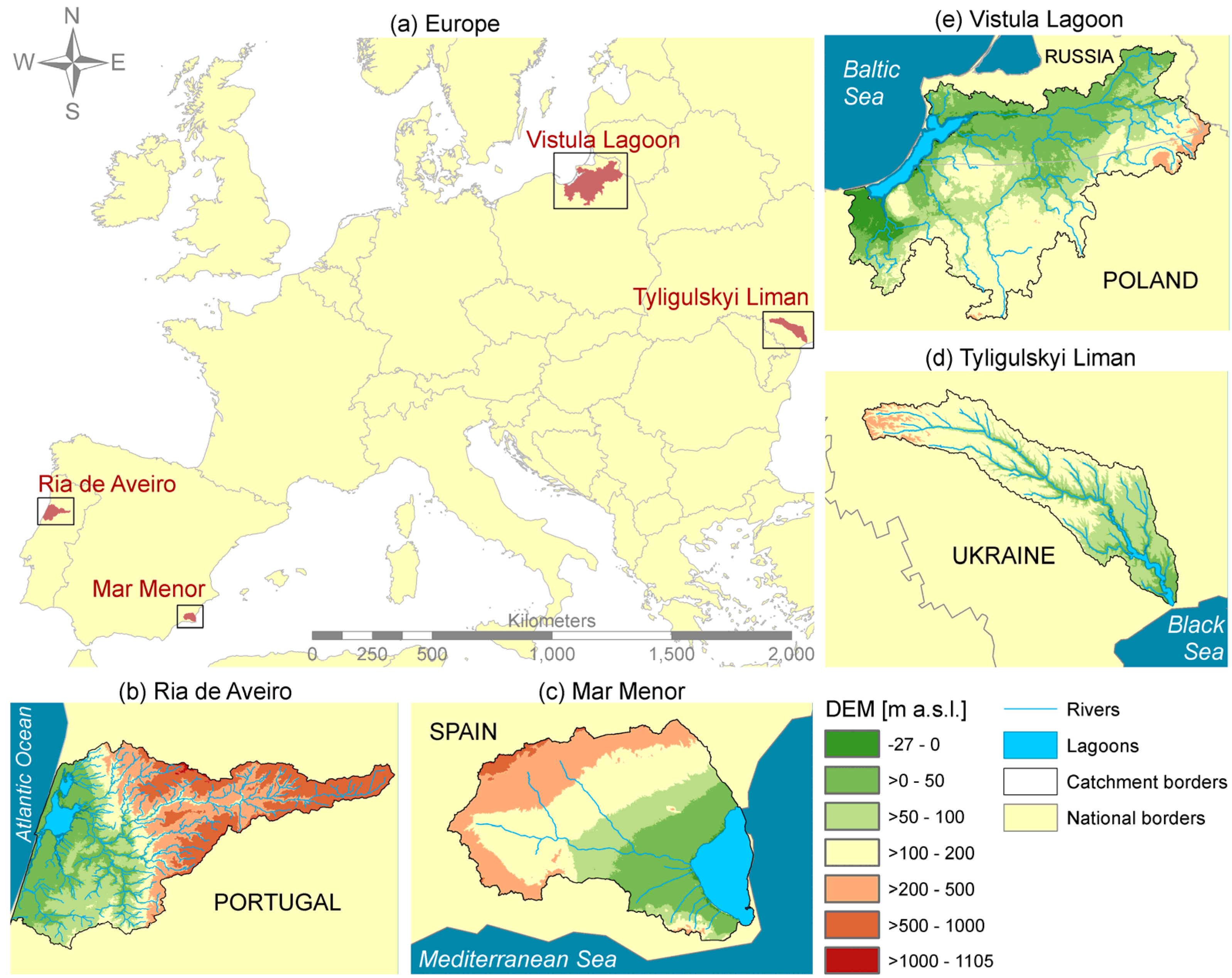
2. Description of the Case Study Areas

Climate and land use change impact assessments were conducted for the catchments of four lagoons located in different regions of Europe and connected to four different seas:

(1): The Ria de Aveiro is located in Portugal and connected to the Atlantic Ocean. It has a catchment of about 3560 km² mainly drained by the Vouga River. The catchment is influenced by a humid and temperate climate, and largely covered by forest.
(2): The Mar Menor is located in Spain close to the Mediterranean Sea with a catchment of about 1380 km². Although the catchment is characterized by hot and dry summers, it is intensively used for irrigated agriculture. The largest river Albujon Wadi often dries up and is not a permanent stream.
(3): The Tyligulskyi Liman can be found in the Ukraine near the Black Sea with a catchment of about 5240 km². It is mainly drained by the Tyligul River and characterized by a warm temperate to continental climate. Due to very fertile soils in this region the catchment is mainly used for agriculture.
(4): The transboundary catchment of the Vistula Lagoon is located in Poland and Russia connected to the Baltic Sea. It covers an area of about 20.730 km² drained by several main rivers in a marine temperate climate. The drainage area is mainly used for agriculture with relatively numerous forested areas.

The locations of the four case study areas (CSA) within Europe as well as the digital elevation models (DEM) for the lagoon catchments can be found in Figure 1. Some catchment characteristics are listed in Table 1.

Figure 1. Location of the four case study areas (CSAs) within Europe (a) as well as the Digital Elevation Models (DEM), locations of lagoons, and main inflowing rivers per CSA (b–e).

The four CSAs investigated in this study are subject to different degrees of human water management impacts on the natural river flow in the catchments. The water management measures in the Aveiro and Vistula Lagoon catchments are not substantial compared to two other cases studies. In relation to the total volume of freshwater inflow to the lagoons, the managed water flows amount to 2.3% in the Ria de Aveiro (abstraction and discharge for public water supply) and 8.5% in the Vistula Lagoon catchment (water transfer from the Vistula River). Additionally, 40% of the Pregolya River discharge does not reach the Vistula Lagoon directly but is instead transferred to another catchment beforehand. However, the management measures are more extensive in the other two cases. In the Mar Menor catchment, the total water inflow to the lagoon is influenced by water transfer from the Tagus catchment (used for irrigation) and the UWTP (urban water treatment plant) effluents (i.e., 51% of the total discharge to the lagoon is related to management). The river discharge in the Tyligulskyi Liman catchment is highly influenced by the construction of ponds within the whole river network and by irretrievable water use (as a result, only 49% of the discharge reaches the lagoon). Therefore, even smaller absolute volumes of water transfer or abstraction can cause a high management degree in catchments with naturally low water discharges, as in the Mar Menor and Tyligulskyi Liman drainage basins, characterized by dry climate conditions.

Table 1. Characteristics of the four case study areas investigated in the study.

**Table 1.** Characteristics of the four case study areas investigated in the study.
Parameter	Unit	Ria de Aveiro	Mar Menor	Tyligulskyi Liman	Vistula Lagoon
Lagoon area	km²	75	135	160	322
Catchment area	km²	3,556	1,380	5,240	20,730
Country(ies)	-	Portugal	Spain	Ukraine	Poland/Russia
Sea	-	Atlantic Ocean	Mediterranean	Black Sea	Baltic Sea
Total freshwater inflow	km³·year⁻¹	2.14	0.009	0.023	3.69
Main inflowing rivers	-	Vouga	Albujon	Tyligul	Pregolya
					Pasleka
					Elblag
Number of analysed inflowing rivers	-	10	7	6	12
Number of infl. rivers with avail. gauge data	-	1	0	1	5
Av. altitude (range)	m a.s.l.	363 (−10–1,105)	100 (−5–1,061)	102 (−6–254)	82 (−27–308)
Av. temperature	°C	14	25	9.7	7.7
Av. precipitation (range)	mm·year⁻¹	1,100 (600–2,100)	337 (300–370)	515 (470–570)	750 (670–860)
Major land uses
Agriculture	%	29	82	80	67
Forest	%	56	1	4	25

3. Material and Methods

3.1. Soil and Water Integrated Model (SWIM)

The eco-hydrological model SWIM [28] was used for climate impact assessment in the four European lagoons. This process-based semi-distributed model was developed based on the models SWAT (Soil Water Assessment Tool) [30] and MATSALU [31] for river basins at the regional scale (200 up to 500,000 km²). The hydrological, nutrient, sediment and vegetation processes are simulated with a daily time step at the hydrotope level. Hydrotopes are sets of the smallest spatial units in SWIM, and are defined as areas within one subbasin with unique land use class and soil type. It is assumed that such units behave similarly regarding water flows, nutrient cycling and vegetation growth (principle of similarity). After process calculation for hydrotopes, the components and flows are aggregated at the subbasin level, and then the lateral flows are routed to the basin’s outlet (and enter the specific lagoon).

Soil hydrological processes in SWIM are based on the water balance equation, and consider surface, subsurface and groundwater flows as well as percolation and recharge of the aquifers. Surface flow is calculated by a non-linear function of precipitation and a retention coefficient which depends on land use, soil type, management, and the actual soil water content. Subsurface flow and percolation are calculated simultaneously, separately for each soil layer: subsurface flow occurs if percolation exceeds field capacity in a layer. The number of soil layers (up to ten can be considered) is defined depending on available soil parameterization for the catchments. Percolation from the bottom soil layer leads to a recharge of the shallow aquifer, from where water can rise again to the soil profile through capillaries, flow laterally to the river network, or percolate to a deep aquifer. From the deep aquifer water cannot rise up again.

Snow processes are simulated using the method of Gelfan et al. [32] as described in Huang [33]. Snow melting is calculated with a degree-day-factor. Water outflow from the snowpack depends on snow depth, content of ice and liquid water, and snow density. The processes of refreezing and snow metamorphism are also considered.

In the original SWIM model potential evapotranspiration is generally calculated based on solar radiation, daily mean temperature and elevation using the method of Priestley and Taylor [34]. However, in the case of the Tyligulskyi Liman catchment the Turc–Ivanov equation [35,36] was used to better reproduce observed values in this catchment. The actual evaporation/transpiration is calculated separately for soils and plants as functions of potential evapotranspiration and the leaf area index (LAI), while soil evaporation is reduced when its accumulated amount exceeds 6 mm. The limited soil water content leads to decreased plant transpiration [28].

Climate as well as land use and management practices are important external drivers for the processes represented in the model. The main external climatic drivers are precipitation and snow fall together with temperature and solar radiation influencing snow melt processes and the evapotranspiration potential of the vegetation and the landscape. Climate parameters are assumed to be homogeneous at the subbasin level. Measured (for model calibration) or projected (for impact assessment) climate data are interpolated to the subbasin centroids by using an inverse weighted distance method.

Due to its spatial resolution as well as climate and land use considered as boundary conditions, the SWIM model allows the analysis of impacts of climate and land use changes on the major model outputs. It is therefore a suitable tool for climate change impact assessments as planned in this study.

SWIM has been successfully applied in several catchments of different sizes firstly in Germany and later in other river basins in Europe, Africa, Asia and South America. It is still being developed further in accordance with the particular research needs or specific case characteristics. An overview of the main applications and implementations can be found in Krysanova et al. [37].

3.2. Input Data, Model Setup and Calibration Strategies

The SWIM model was applied to each of the four case study areas individually. The model setup for the drainage basins of the lagoons was a challenging task, as they mostly consist of several inflowing rivers and streams, with often no available data on water flows and discharges. A non-trivial modelling strategy was necessary to combine several river catchments within one SWIM modelling project for a specific lagoon.

The modelled river discharge could only partly be properly calibrated and validated at one or several gauges in four individual applications, and the sub-catchments of smaller rivers/streams flowing to the lagoons had to be modelled in an ungauged mode. Therefore, calibration and validation were performed for the largest river catchments within the lagoon drainage basins: two in the case of the Vistula Lagoon, and one in each of the three other cases. After that, SWIM was applied for the entire lagoon drainage areas transferring the same calibrated parameters to the ungauged parts, assuming similar geophysical and hydrological conditions in adjacent river catchments but under consideration of catchment-specific characteristics and management settings.

For model setup and hydrological calibration the SWIM model needs spatial data, time series and water management information as input. The spatial data include maps depicting DEM, land use classes and soil type distribution, as well as subbasin structure. The required time series for model setup especially include daily climate data (minimum, maximum and average temperature, precipitation, air humidity and solar radiation). Necessary management data for hydrological modelling include information on water abstraction, water transfer from and to adjacent catchments, major crops with their planting and harvesting dates, as well as irrigation practices on agricultural fields.

Furthermore, river discharge data at gauging stations are needed for model calibration and validation. In three of four catchments, discharge data from several gauges provided an opportunity for a multi-site calibration, which is more reliable in general and especially important in multi-river drainage basins as in our case.

Table 2 presents an overview of datasets used for SWIM application in the drainage basins of the four lagoons. Most of the data are case specific. In all four case study areas some data were missing, or data coverage in time and/or space was problematic. Therefore, in all four cases the model calibration was a very complicated task. The heterogeneity of spatial input data and inconsistent or missing time series of climate and water discharge required interpolation and empirical methods for data estimation.

The model setup and calibration strategies are described in more detail in LAGOONS (2013) as well as the Ria de Aveiro case study area in Stefanova et al. [38] and the Vistula Lagoon case study area in Hesse et al. [39].

During the calibration process, the model results were evaluated in regard to the ability of SWIM to adequately simulate observed water discharges in the lagoon catchments using two criteria of fit: Nash and Sutcliffe efficiency (NSE) and deviation in water balance (DB). The equations to calculate NSE and DB can be found in Hesse et al. [40].

The non-dimensional NSE [41] criterion describes the squared differences between the observed and the simulated values and is based on the dispersion of values around the line of equal values. The NSE can vary from minus infinity to 1 and should be as near as possible to 1. In hydrological modelling, NSE values above 0.5 are considered as corresponding to satisfactory, and above 0.65 as to good modelling results for a monthly time step [42].

Table 2. Data used for model setup and calibration in the catchments of the lagoons under study.

**Table 2.** Data used for model setup and calibration in the catchments of the lagoons under study.
Data	Ria de Aveiro	Mar Menor	Tyligulskyi Liman	Vistula Lagoon
Observed climate	30 stations; large gaps in records; missing solar radiation was derived with the Hargreaves-Samani method	5 stations (4 in the basin), period: 2000–2011	4 climate and 2 precipitation stations outside the catchment available; poor correlation between precipitation and measured discharge → model data for 1979–2009 were used	Observed climate data with poor coverage in time and space → model data for 1979–2009 were used
Observed climate	Sources: http://snirh.pt/ http://www.tutiempo.net/	Source: SIAM	Source: WFDEI climate data [43]	Source: WFDEI climate data [43]
DEM	SRTM (Shuttle Radar Topography Mission)	SRTM (Shuttle Radar Topography Mission)	SRTM (Shuttle Radar Topography Mission)	SRTM (Shuttle Radar Topography Mission)
DEM	Source: http://srtm.csi.cgiar.org/	Source: http://srtm.csi.cgiar.org/	Source: http://srtm.csi.cgiar.org/	Source: http://srtm.csi.cgiar.org/
Land use	CORINE Land Cover 2006, Version 13	CORINE Land Cover 2006, Version 13	No digital data was available A paper map was scanned and digitized	CORINE (CLC2000), Kaliningrad oblast territorial planning scheme
Land use	Source: EEA	Source: EEA	Source: DENR, RDILM	Sources: EEA, PKO
Soil map and soil parameterization	Map: ESDB	Map: HWSD (1 km × 1 km)	Map: HWSD (1 km × 1 km)	Maps: HWSD and SGDBE
Soil map and soil parameterization	Soil parameters from SGDBE and estimated using the German soil mapping guidelines [44]	Soil parameters from HWSD and estimated using the German soil mapping guidelines [44]	Soil parameters from HWSD and estimated using the German soil mapping guidelines [44]	Soil parameters from maps and estimated using the German soil mapping guidelines [44]
Spatial resolution in SWIM	90 m × 90 m raster maps	20 m × 20 m raster maps	100 m × 100 m raster maps	100 m × 100 m raster maps
	365 subbasins	215 subbasins,	175 subbasins	442 subbasins
	2452 hydrotopes	744 hydrotopes	920 hydrotopes	4469 hydrotopes
Observed discharge	hourly/quarterly water levels and flow curve equations for 3 gauges for 2002–2005	no gauge data available, 24 survey measurements for period 09/2003–06/2006, estimated seasonal dynamics for 2003	one upstream gauge (1984–1988) and one downstream gauge (1984–1988 and 1998–2007)	10 discharge gauges for different sub-periods during 1995–2009 Main calibration gauges Lozy (Pasleka river) and Gvardeysk (Pregolya river)
Observed discharge	Source: http://snirh.pt/	Sources: UM, [45,46]	Source: CGO	Sources: IMGW-PIB, KCHEM
Main crops	corn	water melons, lettuce	winter wheat	winter wheat
Main crops	Source: [47]	Source: [48]	Source: [49]	Source: [50]
Water management	Water abstraction: from stream for public water supply with exact location	Irrigation with water from Tagus river (data on annual amounts and location of irrigated area)	Data on ponds and irretrievable water use provided by case study partners	Water inflow and outflow implemented according to literature
Water management	Source: APA	Source: [51]	Sources: IWR-MR, PTR	Sources: [52,53]

Notes: APA—Portuguese Environment Agency (former ARH Centro). CGO—Central Geophysical Observatory http://cgo.kiev.ua. CORINE Land Cover—Coordination of Information on the Environment http://www.eea.europa.eu/data-and-maps/data. DENR—Department of Ecology and Natural Resources, Odessa Regional State Administration http://ecology.odessa.gov.ua/. EEA—European Environment Agency. ESDB/SGDBE—European Soil Database http://eusoils.jrc.ec.europa.eu/data.html. HWSD—Harmonized World Soil Database http://webarchive.iiasa.ac.at/Research/LUC/External-World-soil-database/HTML/. IMGW-PIB—Institute of Meterology and Water Management—National Research Institute. IWR-MR—Inventory of water resources in Mykolaiv Region. Mykolaiv, 2009, pp. 184 (in Ukrainian). KCHEM—Kaliningrad Centre for Meteorology and Environmental Monitoring. PKO—Government of the Kaliningrad Region http://old.gov39.ru/. PTR—Passport of Tyligul River. Odessa: UkrYuzhGIProVodChoz, 1994, pp. 148 (in Russian). RDILM—Odessa Research and Design Institute of Land Management http://www.landres.od.ua/kontakts.html. SIAM—Murcia Agriculture Information System http://siam.imida.es. UM—University Murcia. WFDEI—WATCH Forcing Data methodology applied to ERA-Interim data www.eu-watch.org/publications and ftp.iiasa.ac.at.

The DB criterion corresponds to the percent bias (PBIAS), but with the opposite algebraic sign, and shows the long-term percental difference of the observed values against the simulated ones. For best model results, DB should be as near as possible to 0. In hydrological model applications with a monthly time step, DB/PBIAS below ±25% is considered satisfactory, and DB/PBIAS lower than ±10% shows very good model results [42].

For an objective appraisal of the model results achieved in this study, it should be kept in mind that some criteria of fit presented here were calculated with the daily values, where good performance rates are generally more difficult to obtain than for simulations with the monthly time step.

3.3. Climate Scenario Description and Application

Climate impact assessment in the four lagoon catchments was performed by using a set of climate scenario data provided by the ENSEMBLES project [29]. In this project, a set of RCMs was run using the boundary conditions simulated by different GCMs. All scenarios were driven by the A1B emission scenario, which is an intermediate one concerning projections for increasing atmospheric CO2 concentrations. For the study presented here, only scenarios with the finer spatial resolution of 25 km and a simulation period until the end of the century (mainly until 2098) were selected from the ENSEMBLES climate scenario collection, resulting in a set of 15 different climate scenarios, later referred to as S1 to S15 (Table 3). Such a multi-model approach delivers several projections for the future climate, which have a higher reliability on average than each single scenario with its general uncertainty.

Table 3. Global (GCM) and Regional Climate Model (RCM) combinations and responsible institutes for the 15 ENSEMBLES climate scenarios (S1-S15) used for impact assessment in the case study areas.

**Table 3.** Global (GCM) and Regional Climate Model (RCM) combinations and responsible institutes for the 15 ENSEMBLES climate scenarios (S1-S15) used for impact assessment in the case study areas.
Scenario	GCM	RCM	Institute	Country
S1	HadCM3Q3	RCA3	Swedish Meteorological and Hydrological Institute (SMHI)	Sweden
S2	HadCM3Q0	HadRM3Q0	Hadley Center for Climate Predictions and Research (HC)	Great Britain
S3	HadCM3Q3	HadRM3Q3	Hadley Center for Climate Predictions and Research (HC)	Great Britain
S4	HadCM3Q16	HadRM3Q16	Hadley Center for Climate Predictions and Research (HC)	Great Britain
S5	HadCM3Q16	RCA3	Community Climate Change Consortium for Ireland (4CI)	Northern Ireland
S6	HadCM3Q0	CLM	Swiss Federal Institute of Technology Zurich (ETHZ)	Switzerland
S7	ECHAM5-r3	RACMO2	Royal Netherlands Meteorological Institute (KNMI)	The Netherlands
S8	BCM	RCA3	Swedish Meteorological and Hydrological Institute (SMHI)	Sweden
S9	ECHAM5-r3	RCA3	Swedish Meteorological and Hydrological Institute (SMHI)	Sweden
S10	ECHAM5-r3	REMO	Max Planck Institute for Meteorology (MPI)	Germany
S11	ARPEGE	ALADIN RM5.1	National Center for Meteorological Research (CNRM)	France
S12	ARPEGE	HIRHAM5	Danish Meteorological Institute (DMI)	Denmark
S13	ECHAM5-r3	HIRHAM5	Danish Meteorological Institute (DMI)	Denmark
S14	BCM	HIRHAM5	Danish Meteorological Institute (DMI)	Denmark
S15	ECHAM5-r3	RegCM3	International Center for Theoretical Physics (ICTP)	Italy

As it is a common method in climate impact research to use 30-year-periods [54], scenarios S1 to S15 were divided into the reference period 1971–2000 (p0) and three scenario periods: near future 2011–2040 (p1), intermediate future 2041–2070 (p2), and far future 2071–2098 (p3) for climate impact assessment. They were analysed in advance by comparing the long-term monthly and annual averages of temperature and precipitation and calculating the according climate change signals per future period compared to the reference period of the same scenario (see results in Section 4.2).

The 15 climate scenarios were applied to the calibrated and validated SWIM for the four lagoon drainage basins under investigation. The climate parameters minimum, maximum and average temperature, precipitation, air humidity and solar radiation provided by the 15 individual scenarios were interpolated from the RCM grid points located within or at a maximum distance of 10 km around the catchments to the centroids of the subbasins in every case study area and then used to drive the SWIM model. The basin-specific land use and management input data of the reference period remained unchanged for the future periods in order to evaluate impacts of climate change only.

The climate impacts on runoff in the catchments were analysed considering (1) the long-term average daily, monthly and annual total water inflows to the lagoons; (2) the long-term average annual discharges of the main rivers per CSA; and (3) the long-term average runoff on a map with a hydrotope resolution, and all three analyses averaged over 30 years and 15 scenarios. The results of the three future scenario periods were always compared to the outputs simulated by SWIM under reference conditions driven by the same climate dataset (S1–S15), and not by observed climate. To get an impression of the uncertainty ranges of future projections, different percentiles as well as minimum and maximum values of the scenario results were also analyzed.

4. Results

This section summarizes the results of the study and describes model calibration and validation, presents the climate change signals and impacts on total water inflow to the lagoons and on inflows of separate rivers in the drainage areas with uncertainty estimates. The results section also deals with the impacts on spatial patterns of runoff in the catchment, and concludes with the general climate sensitivity of the total freshwater inflow to the four lagoons under study.

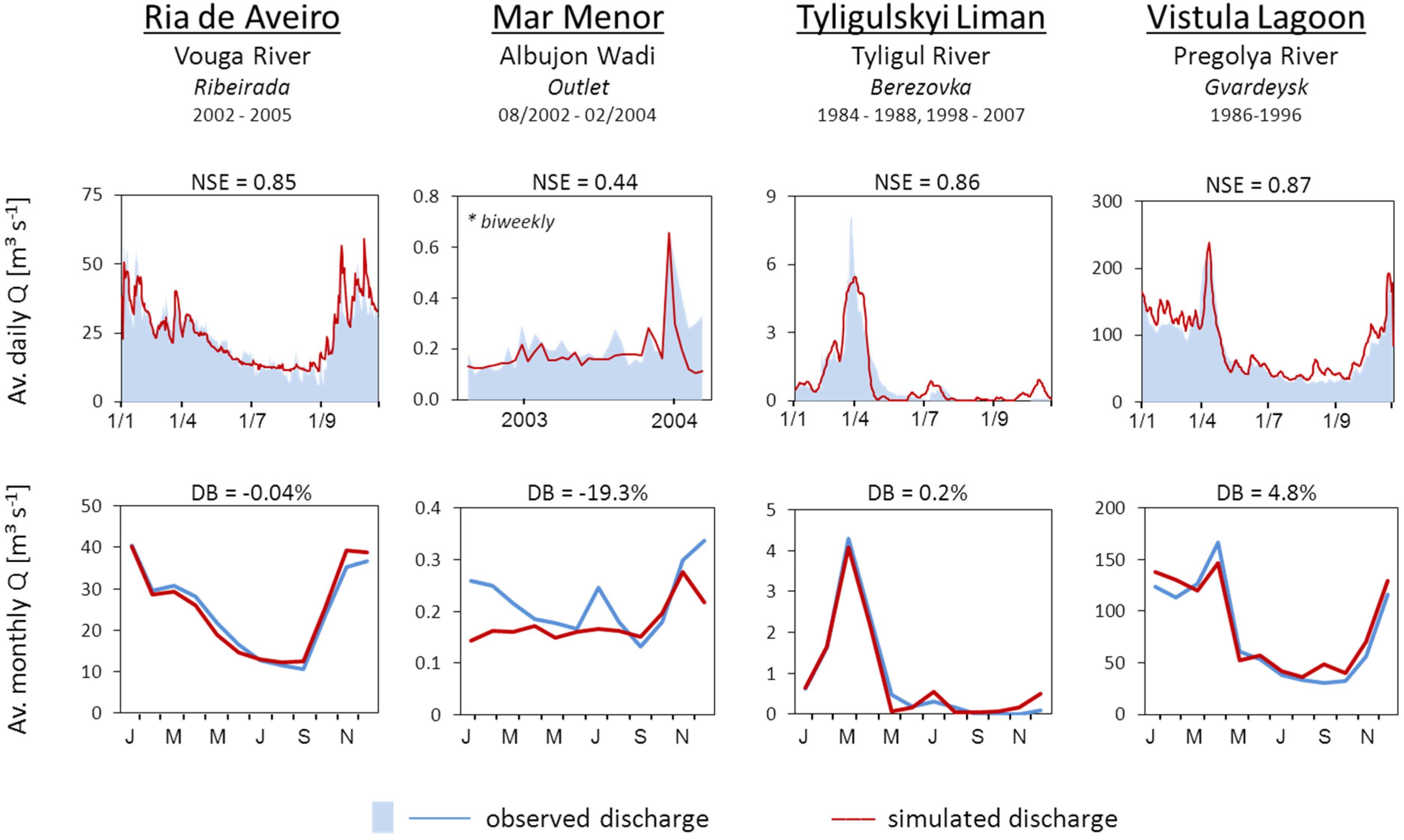
4.1. Model Calibration and Validation in the Four Case Study Areas

A detailed hydrological calibration and validation was performed for three gauges in the Ria de Aveiro catchment, for one gauge in the Mar Menor catchment (using an estimated hydrograph), for two gauges in the Tyligulskyi Liman catchment, and for two gauges in the Vistula Lagoon catchment. Figure 2 shows the observed and simulated long-term average daily and monthly discharges for the most downstream gauging stations of the largest rivers entering each of the four lagoons. In addition, all available discharge data for smaller rivers within the entire lagoon catchments were used for a spatial validation of the calibration parameter set. All analysed gauges are listed in Table 4 together with the criteria of fit achieved there. If available, daily discharge data were used for evaluating model performance, but in some cases only biweekly or monthly values could be compared. The calibration and validation results are presented in more detail in a separate report [55].

Figure 2. Comparison of the long-term average daily and monthly observed and simulated discharges (Q) at selected river gauges in the case study areas. Due to missing daily observed data in the Mar Menor case, the long-term average daily discharge could not be calculated.

Table 4. Criteria of fit achieved at all gauges with available water discharge data applying basin-wide calibration parameter sets in the lagoon case study areas.

**Table 4.** Criteria of fit achieved at all gauges with available water discharge data applying basin-wide calibration parameter sets in the lagoon case study areas.
Catchment	River	Gauge	Period	NSE	DB (%)
Ria de Aveiro	Águeda	Ponte Águeda	2002–2005	0.79	+5.6
	Cértima	Ponte Requeixo	2002–2005	0.72	−19.1
	Vouga	Ribeirada	2002–2005	0.7	−0.04
Mar Menor	Albujon	outlet	8/2002–2/2004 *	0.44	−19
Tyligulskyi Liman	Tyligul	Berezovka	1998–2007 °	0.36	+1.5
		Novoukrainka	1984–1988 °	−0.09	−0.1
		Novoukrainka	1984–1988 ^#	0.86	−0.4
Vistula Lagoon	Angrapa	Berestvo	1995–2000	0.63	−23.6
	Bauda	Nowe Sadulki	2009	0.55	−6.8
	Dzierzgon	Bagart	2009	0.34	−7.4
	Lava	Rodniki	1995–2000	0.70	−7.3
	Mamonovka	Mamonovo	2008–2009 °	0.62	−29.6
	Pasleka	Lozy	2007–2009	0.66	12.9
	Pasleka	Nowa Pasleka	1998–2000 °	0.72	−9.2
	Pissa	Zeleny Bor	1995–2000	0.73	0.4
	Pregolya	Gvardeysk	1983–1996	0.70	0.6
	Waska	Paslek	2009	0.48	−9.8

Notes: * biweekly values.° average monthly values.^# long-term average monthly values.

In the Ria de Aveiro case, hydrological calibration was performed using data from three discharge gauges located within the Vouga catchment, the largest and most important river flowing to the lagoon, one on the main river, and two on tributaries. The observed daily discharges in the Vouga basin were estimated using water levels and unique flow curve equations for each gauge. Since the equations are valid only within certain ranges, some recorded values of very low and very high water levels could not be transformed into daily discharges, which contributed to uncertainty of model calibration in this CSA. The calibration was additionally complicated by human interventions and seasonal damming of water on one tributary, which masks the natural hydrograph. Another large uncertainty is related to missing or incomplete precipitation data in the catchment. Nevertheless, despite all uncertainties in input data, the hydrological calibration of the model was quite successful, reaching NSE values above 0.7 and a relative deviation in water balance of −0.04% at the most downstream gauge Ribeirada (Table 4). The long-term average dynamic of water discharge at this gauge is also reproduced quite well for the calibration period 2002–2005 (Figure 2).

In the Mar Menor catchment, hydrological calibration could not be performed as usual, as there were no observed time series of river discharge available. The calibration was undertaken using biweekly estimated data mainly for 2003 derived from Garcia-Pintado et al. (2007). An additional difficulty was that data on important water contribution to the Albujon Wadi from an urban water treatment plant (UWTP) were not available for 2003, and had to be estimated from the following years. The hydrological cycle in the catchment is additionally influenced by irrigation needs of highly water demanding crops, which are fulfilled by water transfer from adjacent catchments. The calibration results for the period 8/2002–2/2004 using the fortnightly estimated discharge are presented in Figure 2. The simulated curve shows acceptable results. In August 2003 the simulated discharge is missing one peak, which probably has its origin in the discharge coming from the UWTP since almost no rainfall was recorded for this month. Nevertheless, the average simulated discharge for 2003 is 0.20 m³·s⁻¹, which is very close to the 0.24 m³·s⁻¹ estimated by Garcia-Pintado et al. [45].

For the Tyligulskyi Liman catchment data from two gauges located at the Tyligul River, Novoukrainka and Berezovka, were used for hydrological calibration. The calibration was hampered by totally missing data on observed precipitation within the catchment, and poor correlation between observed discharge and precipitation from stations around the catchment. In addition, river discharge is highly influenced by numerous ponds in almost all reaches of the river network, and the high evaporation potential in this region often causing interruption of discharge in summer. The observed discharge could only be reproduced by the model after implementing ponds in the rivers using empirical data. Looking at the long-term average daily and monthly discharges of the Tyligul River (Figure 2) one can see that the model results with NSE of 0.86 and DB of 0.2% are acceptable, and match the average discharge dynamics quite well. However, the comparison of monthly averaged values for two stations (Table 4) shows that the discrepancies between the simulated and observed discharges are still high. The results are better for long-term average discharges, and the achieved DB values indicate that the simulated total water amount coming with the Tyligul River to the lagoon matches the observed values (Table 4). An acceptable balance could also be seen by comparing the simulated outputs with average discharge values from literature for four rivers flowing to the Tyligulskyi Liman as well as for the total inflow to the lagoon [55].

Hydrological calibration of the Vistula Lagoon catchment was a challenging task as well, mainly due to the heterogeneity of spatial input data in this transboundary catchment, and inconsistent time series of observed climate and discharge data with many gaps. The two largest sub-catchments Pregolya (86 m³·s⁻¹ on average) and Pasleka (14 m³·s⁻¹ on average), draining 82% of the total drainage area, were calibrated first, and then the calibrated parameters were used for the whole catchment. The observed and simulated average daily and monthly discharges of the Pregolya are depicted in Figure 2 and show good model performance. Most of the intermediate gauges in the catchment also show satisfactory or good NSE values (Table 4) driven by WFDEI climate data [43], except of the two small rivers Dzierzgon and Waska. These two rivers are located in the lowland area close to the former mouth of the Vistula River, which drains directly into the Baltic Sea now due to hydraulic engineering and rechanneling. The deviation in balance shows good to very good model results in the majority of cases, except two rivers (Angrapa and Mamonovka) with larger discrepancies (Table 4). As the last step in hydrological calibration and spatial validation, average annual data on inflowing water to the lagoon found in literature were compared with the corresponding simulated values at the outlets of the twelve most important rivers entering the Vistula Lagoon [39,55]. In general the results show a good comparison.

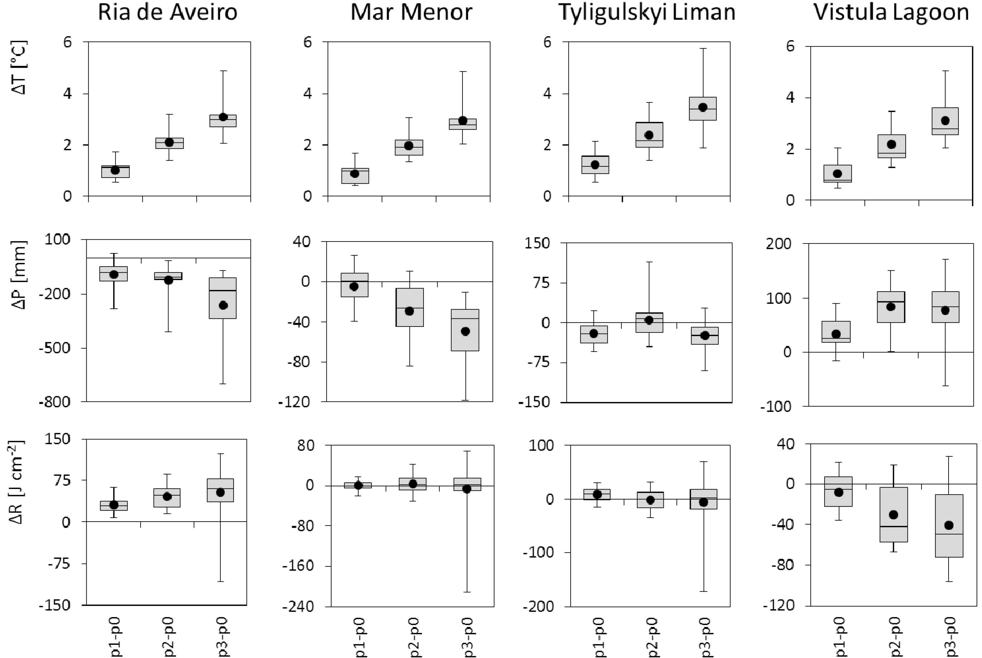
4.2. Climate Change Signals

Climate change signals were calculated as differences in long-term average (30 years) air temperature, precipitation and solar radiation between three future periods p1, p2 and p3 and the reference period p0 averaged over the whole case study areas, separately and averaged over 15 climate scenarios (Table 5).

Table 5. Annual climate change signals of the three future periods p1, p2, and p3 related to the reference period p0 for the parameters air temperature, precipitation and solar radiation averaged over 15 selected ENSEMBLES climate scenarios per lagoon catchment.

**Table 5.** Annual climate change signals of the three future periods p1, p2, and p3 related to the reference period p0 for the parameters air temperature, precipitation and solar radiation averaged over 15 selected ENSEMBLES climate scenarios per lagoon catchment.
Catchment	Temperature (°C)			Precipitation (%)			Radiation (%)
Catchment	p1	p2	p3	p1	p2	p3	p1	p2	p3
Ria de Aveiro	+1.03	+2.1	+3.1	−5.6	−7.5	−15.6	+2.2	+3.3	+3.9
Mar Menor	+0.9	+2.0	+3.0	−1.6	−10.7	−18.3	+0.03	+0.2	−0.3
Tyligulskyi Liman	+1.2	+2.4	+3.5	−3.3	+0.8	−4.1	+0.6	−0.1	−0.4
Vistula Lagoon	+1.1	+2.2	+3.1	+4.3	+10.5	+9.7	−0.8	−3.2	−4.3

The average climate change signals for air temperature show a continuous increase from period p1 to period p3 and are similar for all four case study areas. They amount to 1.06 °C for the period p1, 2.18 °C for p2 and 3.18 °C for p3 on average. For the Tyligulskyi Liman catchment the simulated raise in temperature is higher than for the other three catchments.

Regarding expected changes in precipitation, the change signals are more diverse among the catchments. Until the end of the 21st century, an increasing trend in precipitation is projected for the Vistula Lagoon catchment, while decreasing trends are projected for the Ria de Aveiro and Mar Menor catchments. The strongest relative decrease is simulated for the Mar Menor catchment. For the Tyligulskyi Liman catchment, only very small changes in precipitation are projected on average.

The average change signals for solar radiation show a continuous increasing trend for the Ria de Aveiro catchment, and a decreasing trend for the Vistula Lagoon. Average percental changes in projected solar radiation for the other two catchments are only minor.

However, if single scenarios are analysed, a wide range of possible climate change signals can be seen in the four case study areas (Figure 3). The cases with small changes and without clear trend direction, e.g., for precipitation in the Tyligulskyi Liman catchment or for solar radiation in the Mar Menor and Tyligulskyi Liman catchments, are visible. It can be observed that the projected changes in solar radiation show the opposite change direction than precipitation in the Ria de Aveiro and Vistula Lagoon catchments. Less precipitation means less cloudiness and higher radiation, and vice versa. This connection is less distinct for the other two catchments, which can be probably explained by the influence of some outlying scenarios.

Figure 3. Ranges of climate change signals for 15 ENSEMBLES scenarios calculated as differences in the long-term average annual air temperature (T), precipitation (P) and solar radiation (R) between three future periods (p1, p2, p3) and the reference period (p0). The box plots visualize min/max (error bars), 25/75-percentiles (grey boxes), median (line) and average (dots) values.

In all cases the uncertainty between the 15 ENSEMBLES climate scenarios rises with time, from period p1 to p3. The wide ranges between the minimum and maximum changes are mostly due to outlying scenarios, but the 25/75-percentile boxes cover similar ranges in all three future periods in most cases.

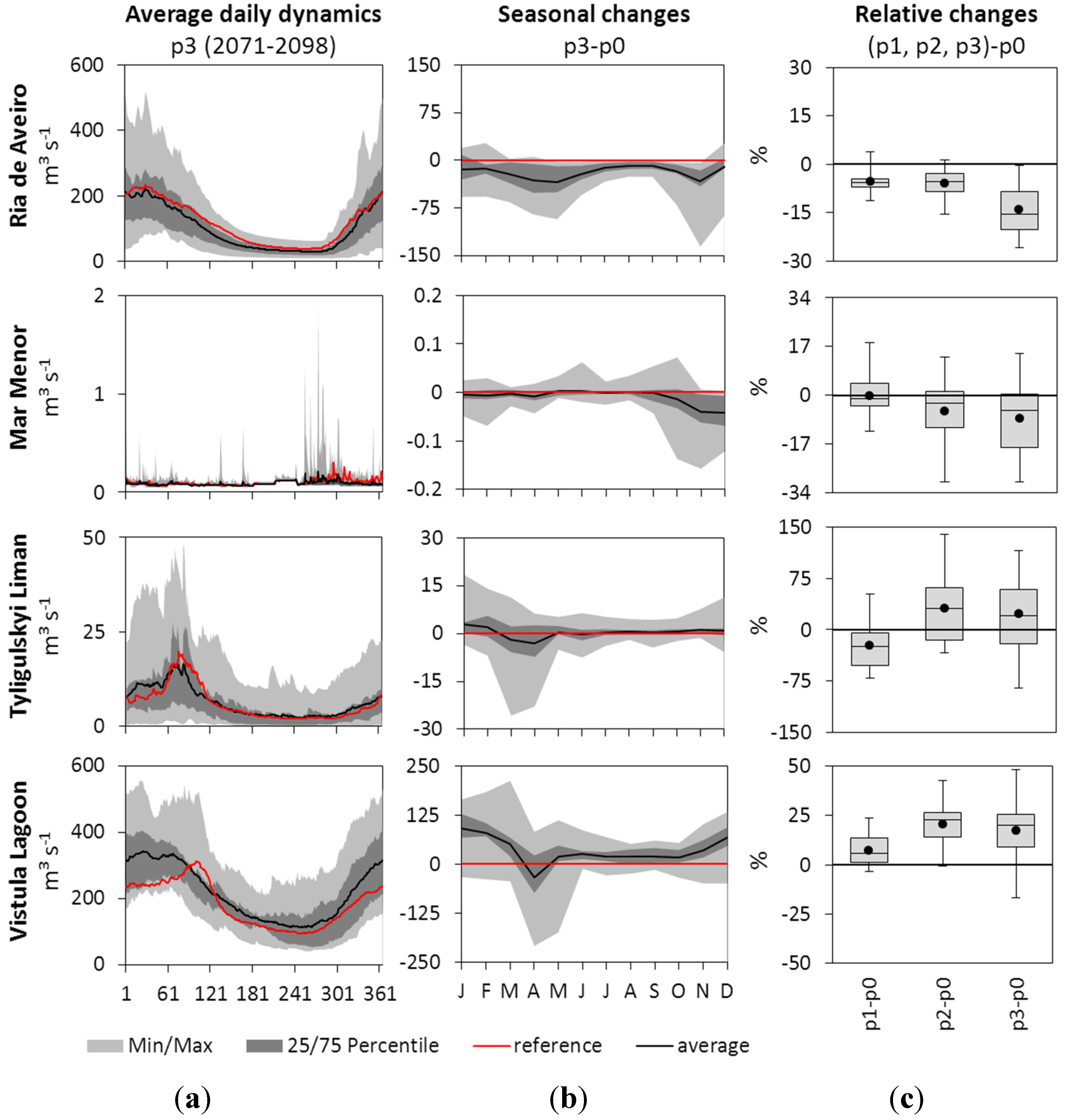
4.3. Impacts of Climate Change on Total Water Discharge to the Lagoons

Figure 4 shows the climate change impacts on total freshwater inputs coming from the catchments to the four lagoons (sum of all inflowing rivers): the long-term average daily dynamics for period p3 (a), the mean monthly differences in total water inflow between periods p3 and p0 (b), and long-term average annual changes for all three future periods compared to the reference period (c). The black line means the average of 15 future scenario simulations, whereas the red line symbolizes the average of 15 simulations driven by climate model data for the reference period p0. The graphs include uncertainty bounds and ranges estimated based on all results driven by 15 climate scenarios and shown by grey shading or, respectively, error bars. The outer light grey uncertainty band is defined by the minimum and maximum outputs, and the dark grey inner band means the 25/75-percentiles of all results. The latter includes 50% of all simulation results around the average and means the range in which freshwater input can be expected in future with a high probability. The results of the future periods were compared with results of the reference period of the same scenario to calculate average monthly and long-term average changes.

Following the precipitation change signal, the simulated long-term average water discharge in the Ria de Aveiro show a moderate decrease in the 1st and 2nd future periods (−5% to −7%), which becomes higher by the end of the century (about −15% on average) (Figure 4, right). Although the decreasing trend is clear on average, there are some scenarios showing a slight increase in the first two scenario periods. The ranges between the 25/75-percentile values (meaning the level of uncertainty for the most probable scenarios) are increasing with time from period p1 to period p3. The projected river discharge to the lagoon in period p3 has a higher uncertainty in the winter months than in the summer season (Figure 4, left). A decrease in average water discharges can be detected during the whole year, while the absolute reduction in spring and autumn is stronger than in summer. Almost all scenarios show the negative trend.

The average climate impacts on freshwater inflow to the Mar Menor are similar to those of Aveiro, as the precipitation change signals have similar trends in these two regions. The results show a moderate decrease of the long-term average discharge to the lagoon by about 10% on average by the end of the century (Figure 4c). For the 1st future period the scenarios do not agree on a common trend and only a negligible decrease on average can be stated. The negative trend becomes more distinct but with a higher uncertainty towards the end of the century. Seasonal changes in water inflow to the Mar Menor show a decrease only in October-December, when generally the highest discharges can be observed (Figure 4b). The absolute uncertainty ranges are quite moderate, as usually water inflow to the lagoon is very low.

The total river discharge to the Tyligulskyi Liman is expected to decline in the scenario period p1, and increase in the two last periods p2 and p3 on average (Figure 4c). These changes do not follow the mean precipitation change signal of the last future period (Figure 3), and can probably be explained by the influence of a decreased solar radiation, which reduces evaporation and by that affects the total discharge. Besides, water inflow to the Tyligulskyi Liman is strongly influenced by water management (ponds), which was considered unchanged in the future in order to investigate “pure” impact of changing climate. The influence of the implemented ponds on the modelled river discharges could interfere with the impacts of a changing climate, and small climate induced changes could be masked. So, only in times when the available water volume exceeds the total effective pond volume in the catchment and evaporation effect on water cycle is low can changes in discharge be observed in future. Looking at the differences in seasonal dynamics of total water inflow to the Liman (Figure 4b), changes can be recognized in winter (an increase) and spring time (a decrease), when warmer winter temperatures influence snowfall and snowmelt processes, which lead to higher winter discharge and earlier and lower snowmelt peak.

Figure 4. Climate change impacts on total freshwater inflow to the four lagoons with uncertainty ranges simulated by SWIM driven by 15 ENSEMBLES scenarios. (a): Long-term average daily dynamics in period p3 (black) with uncertainty ranges (grey) compared to that in the reference period (red); (b): Differences in long-term monthly dynamics between periods p3 and p0 (black) with uncertainty ranges (grey) and zero line (red); (c): Spread of 15 long-term average annual changes for three future periods compared to the reference period of the same scenario. Each box plot visualizes the min/max, 25/75-percentiles, median (line) and average (dot) of 15 average changes. The dynamics for Tyligulskyi Liman are shown without the outlying scenario S8.

The results of climate impact assessment on total inflow to the Vistula Lagoon show a notable increase of 7%, 21% and 18% on average in the three scenario periods due to higher precipitation (Figure 4c). The minimum and maximum ranges projected by SWIM driven by the 15 ENSEMBLES scenarios increase in time from period p1 to p3. The 25/75-percentile ranges (grey boxes) are quite narrow for all three periods, and are located above the zero line. Therefore, an overall increase in future water discharge as simulated by SWIM driven by 15 climate scenarios is quite certain. It can be seen in Figure 4b that positive absolute changes in river discharge are largest in winter and lower in summer. The only negative change in average discharge can be seen in April, probably due to increasing average temperatures causing a totally missing snow melt peak.

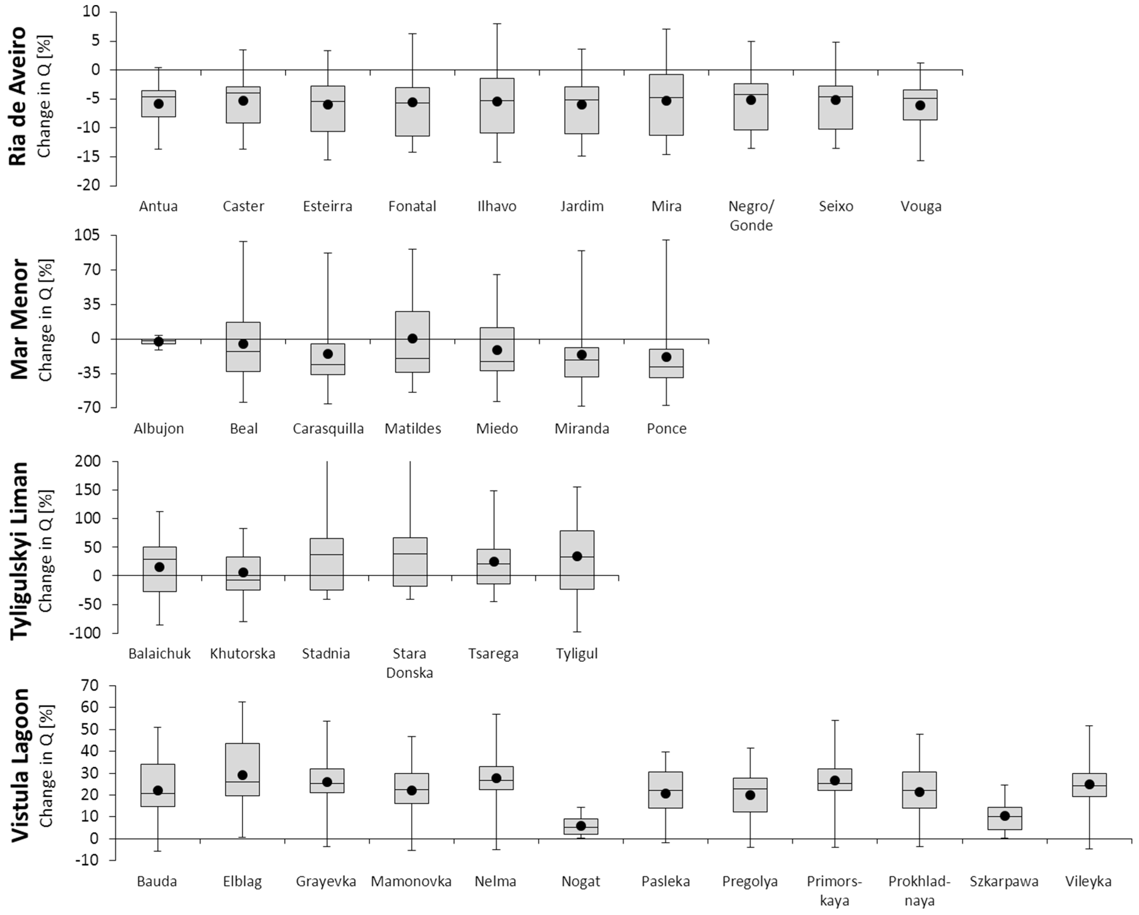
4.4. Impacts of Climate Change on Water Discharge of Single Rivers

Considering the spatial heterogeneity in the four lagoon catchments, it could be assumed that the different rivers and streams entering the lagoons may show different reactions to climate change, depending on the shares of specific land use classes and soil types within their catchments. Therefore, an analysis of climate change impacts was also done for discharges of the individual rivers flowing to the four lagoons. The same as before, percental changes were calculated by comparing the average discharge in the future period with the corresponding value simulated for the reference period of the same scenario. Some selected results comparing the intermediate period p2 with the reference period p0 are shown in Figure 5. This period was chosen, as the expectable future direction of changes should already be clearly visible, but the uncertainty ranges are quite moderate. The box plots show the average and median changes in discharge per river catchment together with their min/max-intervals and the 25/75-percentiles.

In Figure 5 it is evident that the region-specific average trends in total river discharge per CSAs presented in Figure 4 can be detected for the single rivers as well. For the Ria de Aveiro catchment, the majority of 15 climate scenarios project decreasing river discharges in period p2 for all rivers. The decreasing trend is less obvious for the Mar Menor rivers. Mostly an increasing trend with a high uncertainty originating in 15 climate scenarios can be seen for the Tyligulskyi Liman catchment. A distinct increasing trend projected by approximately 90% of the applied climate scenarios is obvious for all rivers flowing to the Vistula Lagoon.

However, some outliers still exist, for example the catchments with the smallest relative changes, e.g., the Albujon Wadi in the Mar Menor catchment, or the Nogat and Szkarpawa Rivers in the Vistula Lagoon catchment, resulting mainly from the water management measures. The effluents from an UWTP (Albujon Wadi) and water transfer from adjacent catchments via the small rivers (Vistula River) implemented in the model mask the climate change impacts in these cases, and result in only small relative changes with narrower uncertainty ranges. The wider uncertainty ranges can be detected in catchments with low or even no flow in drier summer months (e.g., in the smaller Mar Menor or Tyligulskyi Liman tributaries). Here, the relatively high percental changes mean only very low absolute differences in discharge values.

The river-specific analysis of the scenario results shows that the differences in climate impacts on simulated water discharge between the rivers of one catchment can be mostly attributed to the degree of water management within the sub-catchments and less to climate variability or variability in land use and soil distribution. Water management makes the share of natural flow in the rivers considerably smaller and can mask the “pure” climate change impact. But temporally undifferentiated management measures (e.g., water transfer from other catchments, irrigation or waste water outflow from UWTP), which have to be implemented in the model using imprecise information, contribute to the general uncertainty of impact assessment. Additionally, the spatial variability within one (outlying) climate projection or between different climate scenarios can highly influence average results (e.g., for the Tyligulskyi Liman CSA). However, averaging the model outputs driven by a set of scenarios diminishes the influence of a single scenario, and provides more reliable results.

Figure 5. Percental changes in long-term average annual discharge of the main tributaries entering the four lagoons under study comparing the intermediate future period p2 (2041–2070) and the reference period p0 (1971–2000). The box plots visualize min/max, 25/75-percentiles, median (line) and average (dots) values based on simulated results driven by 15 ENSEMBLES scenarios.

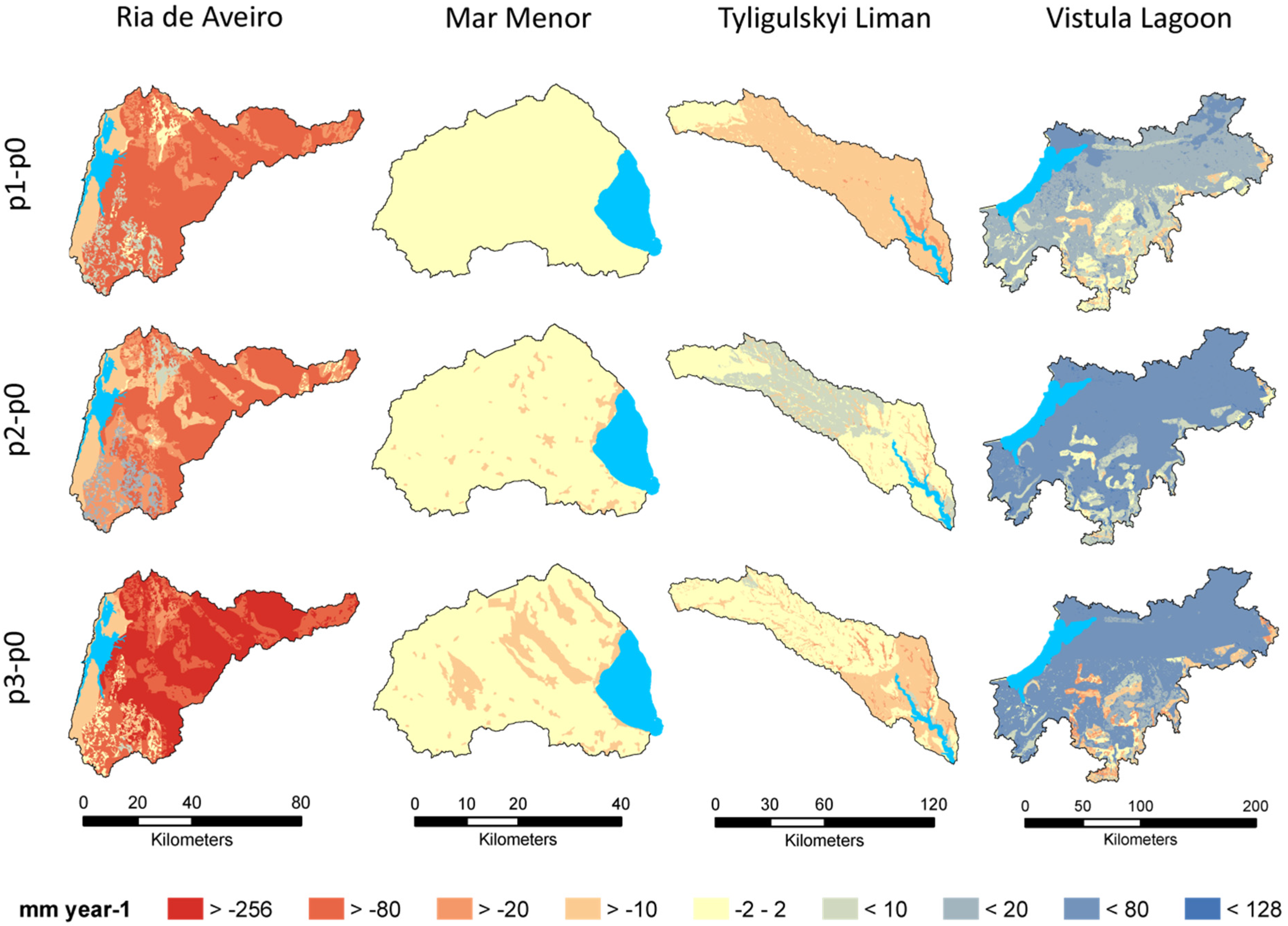
4.5. Impacts of Climate Change on Spatial Patterns of Runoff

Climate change impacts on water flows were additionally analysed in the four lagoon catchments on the hydrotope level to get an impression on the spatial distribution of changes within the catchments. Figure 6 shows the average differences in surface and subsurface runoff between the three future periods and the reference period. For the maps, the annual runoff values per hydrotope were averaged over 30-year-periods for every scenario and over 15 scenarios and then used for calculating and mapping the differences in runoff between periods.

Figure 6. Spatial patterns of average annual changes in runoff (surface and subsurface flow) in the lagoon catchments under study simulated under the set of 15 ENSEMBLES climate change scenarios (average of 15 mean runoff maps for future periods p1, p2, p3 are compared to those of the reference period p0).

The largest average annual decrease in runoff in the Ria de Aveiro catchment is evident for period p3, especially in the eastern part of the catchment with higher elevation. In some areas the average reduction in runoff reaches −250 mm·year⁻¹. However, during the 2nd future period, some areas (agricultural land) show a little increase (6 mm·year⁻¹) due to lower evapotranspiration by affected crops leading to a slightly higher runoff. Besides the land use types, the runoff generation also depends on soil characteristics such as porosity and field capacity. Therefore, different soil types and land use classes can be clearly identified in the runoff maps.

As precipitation and water availability are generally low in the Mar Menor catchment, the average absolute changes in annual runoff are almost not visible in the near future period p1 (< ±1 mm·year⁻¹), and show differences not larger than −10 mm·year⁻¹ in the periods p2 and p3. There are almost no changes visible in the driest western part of the catchment. The highest decrease in runoff can be observed in settlements, which had the highest runoff rates during the reference period, and thus a decrease in precipitation could result in runoff reduction.

Due to the fact that no continuous precipitation trend could be recognized in future in the Tyligulskyi Liman catchment, the spatial patterns of changes in runoff in the three scenario periods are quite diverse. The changes in surface and subsurface runoff more or less reflect the precipitation change signals of the future periods (Figure 3), and show decreasing runoff in the 1st and 3rd periods but practically unchanged or slightly increasing runoff in the 2nd period. They are also influenced by soil type and land use class distributions. The highest decreasing trend in runoff can be observed on areas covered by permanent vegetation (grassland) due to higher evapotranspiration values in these hydrotopes under warmer climate. The simulated decrease is highest in the currently drier south-eastern part of the catchment. It can be concluded that the increase in average discharge (sum of surface, subsurface and groundwater flow) to the Tyligulskyi Liman simulated for the 3rd future period (Figure 4) is probably caused by higher groundwater flow (which is not included in the maps) due to less evapotranspiration with decreased solar radiation.

Looking at the spatial distribution of changes in surface and subsurface runoff in the Vistula Lagoon catchment, the highest average increase is evident in period p2, and the heterogeneity of changes is highest in period p3. The simulated changes in runoff follow the changes in precipitation patterns, but are also influenced by soil characteristics and land use. The runoff increase is lower, or it is even decreasing, on highly permeable soil types, where additional precipitation may contribute to groundwater recharge instead. In general, the simulated changes in runoff are more diverse in the southern Polish part of the catchment, resulting from a soil map with better resolution used for this part of the catchment.

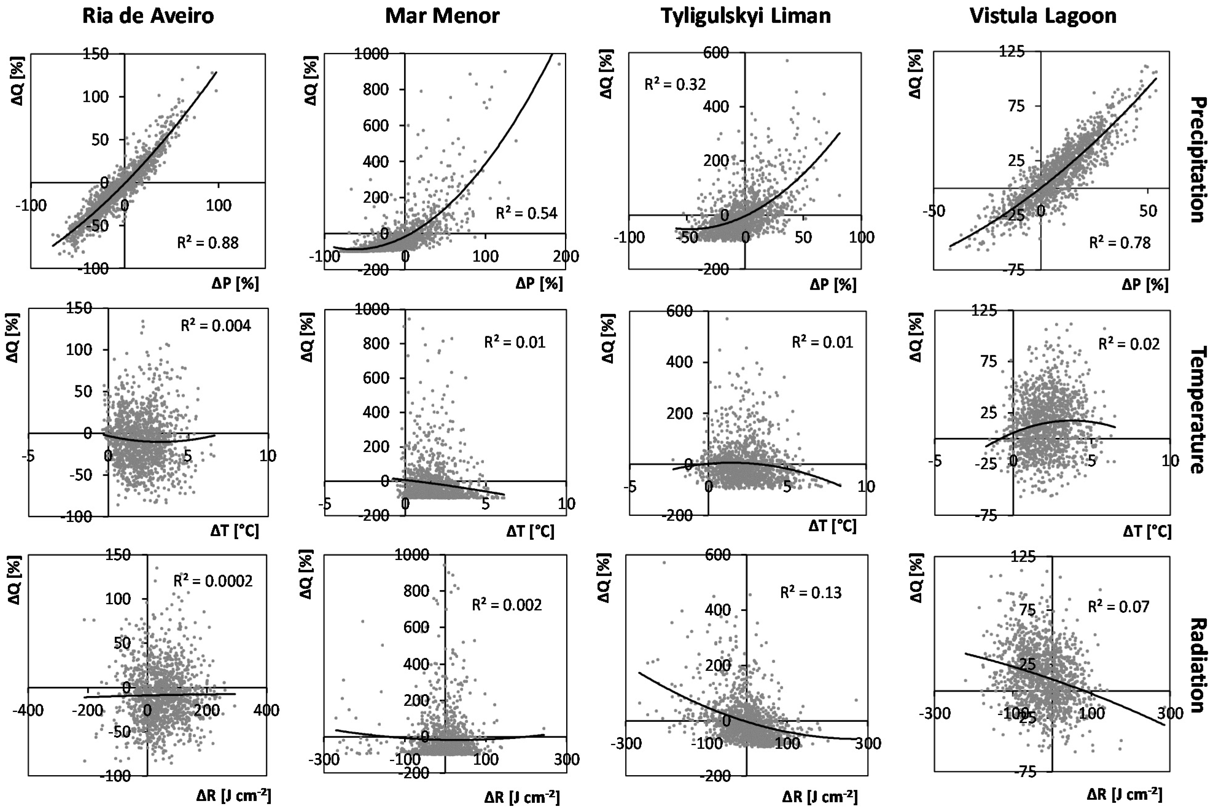
4.6. Climate Sensitivity of Freshwater Inflow to the Lagoons

In addition to the analysis of changes in the long-term average outputs under climate scenarios, the sensitivity of discharge to main climate parameters was analyzed. For that, the relative changes of the annual total water inflow for each future year of the time period 2011–2098 compared to the mean of the reference period 1971–2000 of the same scenario (ΔQ) were plotted against the corresponding relative changes in precipitation (ΔP) or absolute changes in temperature (ΔT) and radiation (ΔR). The latter were estimated the same: as the annual average climate parameters in the time period 2011–2098 related to the means in the reference period 1971–2000 of the same scenario (Figure 7).

Figure 7 illustrates the sensitivity of the total lagoon freshwater inflow (Q) to changes in climate parameters in the four lagoon catchments. The fitted regression curves are plotted as black lines together with their coefficient of determination (R²) to illustrate the correlation between the simulated discharge and climate parameters.

It is evident from Figure 7 that the freshwater inflow is most sensitive to changes in precipitation than to changes in temperature or solar radiation. The highest correlation between Q and P can be seen for the Ria de Aveiro catchment, followed by the Vistula Lagoon, Mar Menor and Tyligulskyi Liman catchments. The degree of correlation is higher in catchments without extensive water management measures (Ria de Aveiro, Vistula Lagoon) and decreases with increasing human impacts on river discharge (Mar Menor, Tyligulskyi Liman).

Figure 7. Climate sensitivity of the total freshwater inflow to the four lagoons for 15 ENSEMBLES climate scenarios: change of modelled annual discharge (ΔQ) per change of annual sum of precipitation (ΔP), average annual temperature (ΔT), and average annual solar radiation (ΔR) for the single years 2011–2098 compared to the mean of the reference period 1971–2000 for the same scenario.

According to the assumed regression lines, positive or negative changes in precipitation by 25% result in different relative changes in total freshwater inflows to the coastal water bodies. The discharge changes per catchment are listed in Table 6. In general, precipitation changes do not cause linear changes in river discharges. Rather, they can be potentiated, especially for catchments with very low natural river discharges and partially dry river beds (Mar Menor, Tyligulskyi Liman). In these catchments, a high number of years can be even detected, where the reduction of precipitation up to 50% causes a full absence of river discharges (−100%). It can be concluded from these experiments that especially water limited ecosystems are highly vulnerable to changing climate conditions.

Table 6. Response of annual modelled discharge to changes in annual sum of precipitation by ± 25%.

**Table 6.** Response of annual modelled discharge to changes in annual sum of precipitation by ± 25%.
Change in Precipitation		+25%	−25%
Resulting change in discharge	Ria de Aveiro	+30%	−25%
	Mar Menor	+50%	−62%
	Tyligulskyi Liman	+61%	−41%
	Vistula Lagoon	+42%	−34%

The coefficients of determination are very low for the relations between discharge and temperature or solar radiation in all catchments (Figure 7). Although higher temperatures and/or radiation should cause an increase in potential evapotranspiration in the catchments and by that influence water inflows, such behaviour is not indicated in the graphs. The largest R² can be seen for the ΔQ/ΔR-ratio in the Tyligulskyi Liman catchment, where decreased solar radiation can affect the resulting water discharge in some years and even mask the average precipitation trend, as already mentioned above in Section 4.3.

5. Discussion

The results of climate change impact assessments for the four European lagoon catchments are in line with the projections described in the literature regarding expected climate change signals and their impacts in Europe. An overall trend in increasing precipitation (especially in winter) for Northern Europe, as well as decreasing precipitation (especially in summer) in the South is mentioned in several publications [4,6,7], and it was also detected in this study. Due to the fact that water limited ecosystems are highly vulnerable to changing climate conditions [56], the robust climate change signals produced by a range of global and regional models suggest that the Mediterranean region and the lagoons located there might be especially vulnerable to climate change [57,58].

The resulting changes in streamflow consequently show an increasing trend in the Northern European Baltic region [59,60], and a decreasing trend around the Mediterranean Sea and on the Iberian Peninsula [61,62]. Comparing with our results on impacts on the water availability in the four lagoon catchments under investigation, the same pattern could be found. Though expected changes in climate can be seen as more beneficial for the Vistula Lagoon catchment, one should not forget about water-related extreme events like floods and drought, which were not explored in this study.

Giorgi and Lionello [57] investigated climate change projections especially for the Mediterranean region. They detected an overall precipitation decrease in this area, but with an inter-seasonal spatial variability due to a shifting transition area between positive (in Northern Europe) and negative (in Southern Europe) precipitation change signals, which moves southward in winter. This could explain the high diversity in precipitation change signals between the 15 ENSEMBLES scenarios for the Tyligulskyi Liman CSA located exactly in this transition zone.

In general, climate change impact assessment performed for the Tyligulskyi Liman catchment reveals the limitations and constraints of the multi-model method for climate impact assessments. If climate input is highly uncertain (as in our case), the eco-hydrological catchment model driven by a set of climate scenarios, showing different directions of change in precipitation and radiation, generates quite heterogeneous model results with high uncertainty ranges, and a clear conclusion for future development is difficult to produce. In addition, as the modelled discharge is highly influenced by anthropogenic water management measures in this region, the ecosystem responses due to “pure” climate change are hardly detectable. Nevertheless, the scenario assessments undertaken in this study helped to identify the direction of potential changes in water quantity in the four lagoon catchments and delivered a first impression about a possible future also for the Tyligulskyi Liman catchment.

However, it cannot be assumed that the results of climate change impact assessment for the four lagoon catchments provide universally valid and strict results, and that impacts projected for a certain scenario (or average projections) will be realised in future. It is common knowledge that even multi-model climate change impact assessments come with some uncertainty [6,63], which should be kept in mind when the results are analysed and interpreted. The uncertainties are mainly related to (A) the ability of climate and eco-hydrological models to represent the interrelated processes in the atmosphere and in a landscape (so-called structural and parametrization uncertainties); (B) the reliability of climate scenarios applied for the impact assessment; and (C) data availability and quality for (eco-)hydrological model setup and calibration. These uncertainties are shortly discussed below.

(A): Models are always simplifications of reality and are characterised by some level of abstraction. Hydrological processes taking place in atmosphere, soils, water bodies and vegetation, as well as interrelations between them, are represented in models with a certain degree of accuracy. This is due to a restricted memory of computers and computation time, as well as due to a limited human knowledge and understanding of processes. Comparing simulated and observed climate data, several studies show the restricted ability of current climate models to satisfactorily reproduce the real local measurements [64,65]. Similar constraints can be found in the hydrological and eco-hydrological models as well. The SWIM model, for example, as a semi-distributed model simulating processes at a hydrotope-level resolution, tries to cover the heterogeneity within a catchment to a certain extent, but is not able to deliver locally exact projections.
(B): A further major uncertainty is connected to climate scenarios applied for impact assessments. Different models come along with different scenarios, and nobody knows the most probable future climate development in a region, as it is influenced by several unpredictable factors. A common method to overcome this problem is to use different scenarios from GCMs and/or RCMs in order to verify most probable projections and investigate ranges of uncertainty. Such method is preferable in comparison with a single climate scenario approach as recommend by many authors [24,25,26,27]. But this procedure still has limitations, and the uncertainty remains high, especially in case of a distinct diversity in climate projections, as detected for the Tyligulskyi Liman catchment in our study.
(C): A hydrological or eco-hydrological model used for an impact assessment should be calibrated and validated in advance. For that, appropriate homogeneous and complete spatial datasets (DEM, land use and soil maps) and time series (daily climate parameters and observed discharge) are necessary for a successful model setup. However, in our case in all four study areas some data were missing, or data coverage in time and/or space was problematic. Therefore, in all four CSAs, the model calibration was a very complicated task (as described in Section 3.2 and Section 4.1), and the model outputs incorporate a certain degree of uncertainty.

Climate scenarios are often customized by applying at least one bias correction method in climate change impact assessment. The bias correction is aimed in avoiding unrealistic simulations of runoff by adjusting the climate scenario data in such a way that they better represent the observed climate. It is still argued whether the application of bias corrected climate scenarios provides better and more reliable results for hydrological impact analyses, especially when relative changes and a detection of trends in runoff are more of interest than the absolute values. While Teutschbein and Seibert [23] recommend the application of bias correction, Ehret et al. [66] state that the bias correction as it is currently used is “not a valid procedure” due to a general lack of the physical justification of corrections, and often missing, incomplete or deficient observed data. In our study it was decided we would not use bias correction, and we would compare simulations driven by 15 RCMs between periods.

6. Summary and Conclusions

The climate change impact assessments for the Ria de Aveiro, Mar Menor, Tyligulskyi Liman and Vistula Lagoon drainage basins were performed by applying a common technique for hydrological impact studies at the catchment scale using a set of 15 climate scenarios provided by the ENSEMBLES project to drive the eco-hydrological model SWIM. Despite some difficulties and uncertainties in model setup and calibration, satisfactory to good model results were achieved, delivering a sound basis for impact assessment. The scenarios covered three future 30-year periods until the end of the 21st century.

The analysis of the 15 scenarios indicates a continuously increasing trend in temperature for all four catchments under investigation. However, precipitation change signals are more diverse between the catchments as well as among the 15 scenarios within one catchment. The highest diversity could be seen for the Tyligulskyi Liman catchment, with only a small change in precipitation on average. A quite consistent increasing trend in precipitation was projected for the Vistula Lagoon catchment, while decreasing trends were projected for the Ria de Aveiro and Mar Menor catchments. The simulated river discharge more or less follows this precipitation pattern and is less sensitive to changes in air temperature or solar radiation. The sensitivity of river discharge to precipitation is more obvious in catchments less influenced by human water management.

The river discharge and flood risk will probably increase in the Vistula Lagoon catchment. In the South-European lagoon catchments, the water managers and stakeholders have to be ready for decreased water availability in the future, and adaptation measures should focus mainly on water-saving technologies. This is particularly important for the very dry Mar Menor catchment with its intensive irrigated agriculture and additional huge water demand in the tourist season. Water availability and freshwater inflow to the lagoon seem to be problematic in the Tyligulskyi Liman area as well. Water flows there are additionally hampered by numerous ponds in the river reaches. Pond management should definitely be adapted to climate change to allow some freshwater inflow to the Liman and prevent its salinization. More consistent and reliable climate scenarios would be desirable for this region in order to reduce uncertainty of projections.

Due to the quite high diversity of climate change impacts detected in the four lagoon catchments under study, it is a challenging task to list valid implications for other coastal areas or lagoon systems in Europe or even worldwide. A variety of lagoons, even in a similar geographical region like the Mediterranean, have a high hydrodynamic and/or saline variability, depending on their morphology and the location and number of river inflows and sea-water inlets influencing the water renewal time [67,68]. Therefore lagoons react differently to climate change with a trend to homogenize hydrodynamic and saline characteristics and to lose hydrodiversity, mainly due to increased inflow of sea water following the sea level rise [17,58]. As northern European lagoons are generally more influenced by river discharge due to the wet climate and the significantly higher runoff coefficients compared to the southern Mediterranean coastal areas [67], climate changes in the lagoon catchments and the resulting changes in river discharge will probably have greater effects on such lagoons fed by permanently flowing rivers than on lagoons located in dry climate.

The results provide some useful insights into possible future water availability and development of freshwater input to the lagoons under study. The model outputs were delivered to the lagoon modellers for evaluating resulting climate change impacts on the lagoon ecosystems. According to the obtained results, impacts are expected to be less pronounced in the near future but would increase in the middle of the century. Consequently, the implementation of adequate adaptation measures in the medium-term is recommended.

However, climate change is not the only factor to have remarkable effects on water resources in the study areas; human societies are important co-designers of the future conditions in these vulnerable coastal areas, too. It cannot be expected that future development will take place without any changes in human behaviour, land use pattern or economic conditions. Therefore, a subsequent combined assessment taking into account possible future climate and socio-economic changes is strongly recommended. This would help to better identify probable future risks and threats, and to virtually test possible adaptation measures as efforts to cope with probable future climate conditions and their impacts.

Acknowledgments

The research leading to these results has received funding from the European Community’s Seventh Framework Programme FP7/2007–2013 through the collaborative research project LAGOONS (contract No. 283157). The ENSEMBLES data used in the study were produced in the EU FP6 Integrated Project ENSEMBLES (contract No. 505539). Hydrological data were provided by several local and national authorities for water management and environmental monitoring in Portugal, Spain, Ukraine, Poland and Russia and collected by the LAGOONS partners, whose support is gratefully acknowledged. The authors thank Vanessa Wörner and Lasse Scheele for their support in climate scenario data download, preparation and evaluation.

Author Contributions

All authors planned and designed the methods to study climate change impacts on water resources in the four case study areas. Cornelia Hesse set up, adjusted and calibrated the SWIM model for the Tyligulskyi Liman and Vistula Lagoon catchments and ran the scenarios for these two CSAs. Anastassi Stefanova set up, adjusted and calibrated the model for the Ria de Aveiro and Mar Menor catchments and ran the scenarios for these two CSAs. Cornelia Hesse and Anastassi Stefanova analyzed the model output data. Cornelia Hesse analyzed the climate sensitivity and impacts on single rivers, prepared all tables and figures for the publication, wrote the text and formatted the paper. Valentina Krysanova guided and supervised the whole process, discussed results during the modelling study, and edited the manuscript.

Conflicts of Interest

The authors declare no conflict of interest.

References

IPCC Summary for Policymakers. In Climate Change 2007: Impacts, Adaptation and Vulnerability. Contribution of Working Group II to the Fourth Assessment Report of the Inter-governmental Panel on Climate Change; Parry, M.L.; Canziani, O.F.; Palutikof, J.P.; van der Linden, P.J.; Hanson, C.E. (Eds.) Cambridge University Press: Cambridge, UK, 2007; pp. 7–22.
IPCC Summary for Policymakers. In Climate Change 2013: The Physical Science Basis. Contribution of Working Group I to the Fifth Assessment Report of the Intergovernmental Panel on Climate Change; Stocker, T.F.; Qin, D.; Plattner, G.-K.; Tignor, M.; Allen, S.K.; Boschung, J.; Nauels, A.; Xia, Y.; Bex, V.; Midgley, P.M. (Eds.) Cambridge University Press: Cambridge, UK, 2013; pp. 3–29.
Kundzewicz, Z.W. Climate change impacts on the hydrological cycle. Ecohydrol. Hydrobiol. 2008, 8, 195–203. [Google Scholar] [CrossRef]
Cassardo, C.; Jones, J.A.A. Managing water in a changing world. Water 2011, 3, 618–628. [Google Scholar] [CrossRef]
Kløve, B.; Ala-Aho, P.; Bertrand, G.; Gurdak, J.J.; Kupfersberger, H.; Kværner, J.; Muotka, T.; Mykrä, H.; Preda, E.; Rossi, P.; et al. Climate change impacts on groundwater and dependent ecosystems. J. Hydrol. 2014, 518, 250–266. [Google Scholar]
European Environment Agency (EEA). Climate Change, Impacts and Vulnerability in Europe 2012; EEA-Report No 12/2012; European Environment Agency: Copenhagen, Denmark, 2012; p. 300. [Google Scholar] [CrossRef]
Alcamo, J.; Moreno, J.M.; Nováky, B.; Bindi, M.; Corobov, R.; Devoy, R.J.N.; Giannakopoulos, C.; Martin, E.; Olesen, J.E.; Shvidenko, A. Europe. In Climate Change 2007: Impacts, Adaptation and Vulnerability; Contribution of Working Group II to the Fourth Assessment Report of the Intergovernmental Panel on Climate Change; Parry, M.L., Canziani, O.F., Palutikof, J.P., van der Linden, P.J., Hanson, C.E., Eds.; Cambridge University Press: Cambridge, UK, 2007; pp. 541–580. [Google Scholar]
Haylock, M.R.; Hofstra, N.; Klein Tank, A.M.G.; Klok, E.J.; Jones, P.D.; New, M. A European daily high-resolution gridded data set of surface temperature and precipitation for 1950–2006. J. Geophys. Res. 2008, 113. [Google Scholar] [CrossRef]
Linderholm, H.W. Growing season changes in the last century. Agric. For. Meteorol. 2006, 137, 1–14. [Google Scholar] [CrossRef]
Gabriel, K.M.A.; Endlicher, W.R. Urban and rural mortality rates during heat waves in Berlin and Brandenburg, Germany. Environ. Pollut. 2011, 159, 2044–2050. [Google Scholar] [CrossRef] [PubMed]
Vittoz, P.; Cherix, D.; Gonseth, Y.; Lubini, V.; Maggini, R.; Zbinden, N.; Zumbach, S. Climate change impacts on biodiversity in Switzerland: A review. J. Nat. Conserv. 2013, 21, 154–162. [Google Scholar] [CrossRef]
Wang, X.; Siegert, F.; Zhou, A.; Franke, J. Glacier and glacial lake changes and their relationship in the context of climate change, Central Tibetan Plateau 1972–2010. Glob. Planet. Chang. 2013, 111, 246–257. [Google Scholar] [CrossRef]
Nicholls, R.J.; Wong, P.P.; Burkett, V.R.; Codignotto, J.O.; Hay, J.E.; McLean, R.F.; Ragoonaden, S.; Woodroffe, C.D. Coastal systems and low-lying areas. In Climate Change 2007: Impacts, Adaptation and Vulnerability. Contribution of Working Group II to the Fourth Assessment Report of the Inter-Governmental Panel on Climate Change; Parry, M.L., Canziani, O.F., Palutikof, J.P., van der Linden, P.J., Hanson, C.E., Eds.; Cambridge University Press: Cambridge, UK, 2007; pp. 315–356. [Google Scholar]
National Research Council (NRC). Adapting to the Impacts of Climate Change; The National Academies Press: Washington, DC, USA, 2010; p. 292. [Google Scholar]
Anthony, A.; Atwood, J.; August, P.; Byron, C.; Cobb, S.; Foster, C.; Fry, C.; Gold, A.; Hagos, K.; Heffner, L.; et al. Coastal lagoons and climate change: Ecological and social ramifications in U.S. Atlantic and Gulf coast ecosystems. Ecol. Soc. 2009, 14, p. 8. Available online: http://www.ecologyandsociety.org/vol14/iss1/art8/ (accessed on 3 December 2013).
Chapman, P.M. Management of coastal lagoons under climate change. Estuar. Coast. Shelf Sci. 2012, 110, 32–35. [Google Scholar] [CrossRef]
De Pascalis, F.; Pérez-Ruzafa, A.; Gilabert, J.; Marcos, C.; Umgiesser, G. Climate change response of the Mar Menor coastal lagoon (Spain) using a hydrodynamic finite element model. Estuar. Coast. Shelf Sci. 2012, 114, 118–129. [Google Scholar] [CrossRef]
Scavia, D.; Field, J.C.; Boesch, D.F.; Buddemeier, R.W.; Burkett, V.; Cayan, D.R.; Fogarty, M.; Harwell, M.A.; Howarth, R.W.; Mason, C.; et al. Climate change impacts on U.S. coastal and marine ecosystems. Estuaries 2002, 25, 149–164. [Google Scholar]
Jakimavicius, D.; Kriauciuniene, J. The Climate change impact on the water balance of the curonian lagoon. Water Resour. 2013, 40, 120–132. [Google Scholar] [CrossRef]
Hirabayashi, Y.; Kanae, S.; Emori, S.; Oki, T.; Kimoto, M. Global projections of changing risk of floods and droughts in a changing climate. Hydrolog. Sci. J. 2008, 53, 754–772. [Google Scholar] [CrossRef]
Arnell, N.W.; Gosling, S.N. The impacts of climate change on river flow regimes at the global scale. J. Hydrol. 2013, 486, 351–364. [Google Scholar] [CrossRef]
Van Vliet, M.T.H.; Franssen, W.H.P.; Yearsley, J.R.; Ludwig, F.; Haddeland, I.; Lettenmaier, D.P.; Kabat, P. Global river discharge and water temperature under climate change. Glob. Environ. Chang. 2013, 23, 450–464. [Google Scholar] [CrossRef]
Teutschbein, C.; Seibert, J. Regional climate models for hydrological impact studies at the catchment scale: A review of recent modeling strategies. Geogr. Compass 2010, 4, 834–860. [Google Scholar] [CrossRef] [Green Version]
Giorgi, F.; Hewitson, B.; Christensen, J.H.; Hulme, M.; von Storch, H.; Whetton, P.; Jones, R.; Mearns, L.; Fu, C. Regional climate information—Evaluation and projections. In Climate Change 2001: The Scientific Basis; Contribution of Working Group I to the Third Assessment Report of the Intergovernmental Panel on Climate Change; Houghton, J.T., Ding, Y., Griggs, D.J., Noguer, M., van der Linden, P.J., Dai, X., Maskell, K., Johnson, C.A., Eds.; Cambridge University Press: Cambridge, UK, 2001; pp. 583–638. [Google Scholar]
Fowler, H.; Blenkinsop, S.; Tebaldi, C. Linking climate change to impact studies: Recent advances in downscaling techniques for hydrological modelling. Int. J. Climatol. 2007, 27, 1547–1578. [Google Scholar] [CrossRef]
Graham, L.; Andreasson, J.; Carlsson, B. Assessing climate change impacts on hydrology from an ensemble of regional climate models, model scales and linking methods—A case study on the Lule river basin. Clim. Chang. 2007, 81, 293–307. [Google Scholar] [CrossRef]
Tebaldi, C.; Knutti, R. The use of the multi-model ensemble in probabilistic climate projections. Philos. Trans. R. Soc. 2007, 365, 2053–2075. [Google Scholar] [CrossRef]
Krysanova, V.; Wechsung, F.; Arnold, J.; Srinivasan, R.; Williams, J. SWIM (Soil and Water Integrated Model): User Manual; PIK Report No. 69; Potsdam Institute for Climate Impact Research (PIK): Potsdam, Germany, 2000; p. 239. [Google Scholar]
ENSEMBLES: Climate Change and Its Impacts: Summary of Research and Results from the ENSEMBLES Project; Van der Linden, P.; Mitchell, J.F. (Eds.) Met Office Hadley Centre: Exeter, UK, 2009; p. 160.
Arnold, J.; Allan, P.; Bernhardt, G. A comprehensive surface-groundwater flow model. J. Hydrol. 1993, 142, 47–69. [Google Scholar] [CrossRef]
Krysanova, V.; Meiner, A.; Roosaare, J.; Vasilyev, A. Simulation modelling of the coastal waters pollution from agricultural watershed. Ecol. Model. 1989, 49, 7–29. [Google Scholar] [CrossRef]
Gelfan, A.; Poneroy, J.; Kuchment, L. Modelling forest cover influences on snow accumulation, sublimation, and melt. J. Hydrometeorol. 2004, 5, 785–803. [Google Scholar] [CrossRef]
Huang, S. Modelling of Environmental Change Impacts on Water Resources and Hydrological Extremes in Germany. Ph.D. Thesis, University Potsdam, Potsdam, Germany, November 2011; p. 206. [Google Scholar]
Priestley, C.; Taylor, R. On the assessment of surface heat flux and evaporation using large scale parameters. Mon. Weather Rev. 1972, 100, 81–92. [Google Scholar] [CrossRef]
Turc, L. Évaluation des besoins en eau d’irrigation, évapotranspiration potentielle, formule simplifiée et mise à jour. Ann. Agron. 1961, 12, 13–49. (In French) [Google Scholar]
Wendling, U.; Schellin, H. Neue Ergebnisse zur Berechnung der potentiellen Evapotranspiration. Z. Meteorol. 1986, 36, 214–217. (In German) [Google Scholar]
Krysanova, V.; Hattermann, F.F.; Huang, S.; Hesse, C.; Vetter, T.; Liersch, S.; Koch, H.; Kundzewicz, Z. Modelling climate and land-use change impacts with SWIM: Lessons learnt from multiple applications. Hydrol. Sci. J. 2014. [Google Scholar] [CrossRef]
Stefanova, A.; Krysanova, V.; Hesse, C.; Lillebø, A. Climate change impact assessment on water inflow to a coastal lagoon: Ria de Aveiro watershed, Portugal. Hydrol. Sci. J. 2014. [Google Scholar] [CrossRef]
Hesse, C.; Krysanova, V.; Stefanova, A.; Bielecka, M.; Domnin, D. Assessment of climate change impacts on water quantity and quality of the multi-river Vistula Lagoon catchment. Hydrol. Sci. J. 2014. [Google Scholar] [CrossRef]
Hesse, C.; Krysanova, V.; Päzolt, J.; Hattermann, F.F. Eco-hydrological modelling in a highly regulated lowland catchment to find measures for improving water quality. Ecol. Model. 2008, 218, 135–148. [Google Scholar] [CrossRef]
Nash, J.E.; Sutcliffe, J.V. River flow forecasting through conceptual models part I: A discussion of principles. J. Hydrol. 1970, 10, 282–290. [Google Scholar] [CrossRef]
Moriasi, D.N.; Arnold, J.G.; van Liew, M.W.; Bingner, R.L.; Harmel, R.D.; Veith, T.L. Model Evaluation guidelines for systematic quantification of accuracy in watershed simulations. Trans. ASABE 2007, 50, 885–900. [Google Scholar] [CrossRef]
Weedon, G.P.; Balsamo, G.; Bellouin, N.; Gomes, S.; Best, M.J.; Viterbo, P. The WFDEI meteorological forcing data set: Watch forcing data methodology applied to ERA-interim reanalysis data. Water Resour. Res. 2014, 50. [Google Scholar] [CrossRef]
Bodenkundliche Kartieranleitung, 5th ed.; Boden AG: Hannover, Germany, 2005; p. 392.
García-Pintado, J.; Martínez-Mena, M.; Barberá, G.G.; Albaladejo, J.; Castillo, V.M. Anthropo-genic nutrient sources and loads from a Mediterranean catchment into a coastal lagoon: Mar Menor, Spain. Sci. Total Environ. 2007, 373, 220–239. [Google Scholar] [CrossRef] [PubMed]
Velasco, J.; Lloret, J.; Millán, A.; Marín, A.; Barahona, J.; Abellán, P.; Sánchez-Fernández, D. Nutrient and particulate inputs into the Mar Menor lagoon (SE Spain) from an intensive agricultural watershed. Water Air Soil Pollut. 2006, 176, 37–56. [Google Scholar] [CrossRef]
The Ria de Aveiro Lagoon—Current Knowledge Base and Knowledge Gaps; LAGOONS Report D2.1b; UA: Aveiro, Portugal, 2012; p. 52.
Jimenez-Martinez, J.; Skaggs, T.H.; van Genuchten, M.T.; Candela, L. A root zone modelling approach to estimating groundwater recharge from irrigated areas. J. Hydrol. 2009, 367, 138–149. [Google Scholar] [CrossRef]
The Tyligulskyi Lagoon—Current Knowledge Base and Knowledge Gaps; LAGOONS Report D2.1d; OSENU: Odessa, Ukraine, 2012; p. 54.
Eriksson, H.; Pastuszak, M.; Löfgren, S.; Mörth, C.-M.; Humborg, C. Nitrogen budgets of the Polish agriculture 1960–2000: Implications for riverine nitrogen loads to the Baltic Sea from transitional countries. Biogeochemistry 2007, 85, 153–168. [Google Scholar] [CrossRef]
The Mar Menor Lagoon—Current Knowledge Base and Knowledge Gaps; LAGOONS Report D2.1c; UM: Murcia, Spain, 2012; p. 65.
The Vistula Lagoon—Current Knowledge Base and Knowledge Gaps; LAGOONS Report D2.1a; IBW-PAN: Gdansk, Poland, 2012; p. 99.
Robakiewicz, M. Vistula River mouth—History and recent problems. Arch. Hydro–Eng. Environ. Mech. 2012, 57, 155–166. [Google Scholar]
Guidelines on the Use of Scenario Data for Climate Impact and Adaptation Assessment, 1st ed.; Carter, T.R.; Hulme, M.; Lal, M. (Eds.) Intergovernmental Panel on Climate Change, Task Group on Scenarios for Climate Impact Assessment (IPCC-TGCIA): Helsinki, Finland, 1999.
Results of Climate Impact Assessment—Application for Four Lagoon Catchments; LAGOONS Report D5.1; PIK: Potsdam, Germany, 2013; p. 107.
Manfreda, S.; Caylor, K.K. On the vulnerability of water limited ecosystems to climate change. Water 2013, 5, 819–833. [Google Scholar] [CrossRef]
Giorgi, F.; Lionello, P. Climate change projections for the Mediterranean region. Glob. Planet. Chang. 2008, 63, 90–104. [Google Scholar] [CrossRef]
Ferrarin, C.; Bajo, M.; Bellafiore, D.; Cucco, A.; de Pascalis, F.; Ghezzo, M.; Umgiesser, G. Toward homogenization of Mediterranean lagoons and their loss of hydrodiversity. Geophys. Res. Lett. 2014, 41, 5935–5941. [Google Scholar] [CrossRef]
Graham, L. Climate change effects on river flow to the Baltic Sea. AMBIO 2004, 33, 235–241. [Google Scholar] [PubMed]
Reihan, A.; Koltsova, T.; Kriauciuniene, J.; Lizuma, L.; Meilutyte-Barauskiene, D. Changes in water discharge of the Baltic States Rivers in the 20th century and its relation to climate change. Nord. Hydrol. 2007, 38, 401–412. [Google Scholar] [CrossRef]
García-Ruiz, J.M.; López-Moreno, J.I.; Vicente-Serrano, S.M.; Lasanta-Martínez, T.; Beguería, S. Mediterranean water resources in a global change scenario. Earth Sci. Rev. 2011, 105, 121–139. [Google Scholar] [CrossRef] [Green Version]
Arias, R.; Rodriguez-Blanco, M.L.; Taboada-Castro, M.M.; Nunes, J.P.; Keizer, J.J.; Taboada-Castro, M.T. Water resources response to changes in temperature, rainfall and CO₂ concentration: A first approach in NW Spain. Water 2014, 6, 3049–3067. [Google Scholar] [CrossRef]
Koutsoyiannis, D.; Efstratiadis, A.; Mamassis, N.; Christofides, A. On the credibility of climate predictions. Hydrol. Sci. J. 2008, 53, 671–684. [Google Scholar] [CrossRef]
Anagnostopoulos, G.G.; Koutsoyiannis, D.; Christofides, A.; Efstratiadis, A.; Mamassis, N. A comparison of local and aggregated climate model outputs with observed data. Hydrol. Sci. J. 2010, 55, 1094–1110. [Google Scholar] [CrossRef]
Kundzewicz, Z.W.; Stakhiv, E.Z. Are climate models “ready for prime time” in water resources management applications, or is more research needed? Hydrolog. Sci. J. 2010, 55, 1085–1089. [Google Scholar] [CrossRef]
Ehret, U.; Zehe, E.; Wulfmeyer, V.; Warrach-Sagi, K.; Liebert, J. HESS Opinions “Should we apply bias correction to global and regional climate model data? ” Hydrol. Earth Syst. Sci. 2012, 16, 3391–3404. [Google Scholar] [CrossRef]
Newton, A.; Icely, J.; Cristina, S.; Brito, A.; Cardoso, A.C.; Colijn, F.; Riva, S.D.; Gertz, F.; Hansen, J.W.; Holmer, M.; et al. An overview of ecological status, vulnerability and future perspectives of European large shallow, semi-enclosed coastal systems, lagoons and transitional waters. Estuar. Coast. Shelf Sci. 2014, 140, 95–122. [Google Scholar] [CrossRef]
Umgiesser, G.; Ferrarin, C.; Cucco, A.; de Pascalis, F.; Bellafiore, D.; Ghezzo, M.; Bajo, M. Comparative hydrodynamics of 10 Mediterranean lagoons by means of numerical modelling. J. Geophys. Res. Oceans 2014, 119, 2212–2226. [Google Scholar] [CrossRef]

© 2015 by the authors; licensee MDPI, Basel, Switzerland. This article is an open access article distributed under the terms and conditions of the Creative Commons Attribution license (http://creativecommons.org/licenses/by/4.0/).

Share and Cite

MDPI and ACS Style

Hesse, C.; Stefanova, A.; Krysanova, V. Comparison of Water Flows in Four European Lagoon Catchments under a Set of Future Climate Scenarios. Water 2015, 7, 716-746. https://doi.org/10.3390/w7020716

AMA Style

Hesse C, Stefanova A, Krysanova V. Comparison of Water Flows in Four European Lagoon Catchments under a Set of Future Climate Scenarios. Water. 2015; 7(2):716-746. https://doi.org/10.3390/w7020716

Chicago/Turabian Style

Hesse, Cornelia, Anastassi Stefanova, and Valentina Krysanova. 2015. "Comparison of Water Flows in Four European Lagoon Catchments under a Set of Future Climate Scenarios" Water 7, no. 2: 716-746. https://doi.org/10.3390/w7020716

Article Menu

Comparison of Water Flows in Four European Lagoon Catchments under a Set of Future Climate Scenarios

Abstract

1. Introduction

2. Description of the Case Study Areas

3. Material and Methods

3.1. Soil and Water Integrated Model (SWIM)

3.2. Input Data, Model Setup and Calibration Strategies

3.3. Climate Scenario Description and Application

4. Results

4.1. Model Calibration and Validation in the Four Case Study Areas

4.2. Climate Change Signals

4.3. Impacts of Climate Change on Total Water Discharge to the Lagoons

4.4. Impacts of Climate Change on Water Discharge of Single Rivers

4.5. Impacts of Climate Change on Spatial Patterns of Runoff

4.6. Climate Sensitivity of Freshwater Inflow to the Lagoons

5. Discussion

6. Summary and Conclusions

Acknowledgments

Author Contributions

Conflicts of Interest

References

Share and Cite

Article Metrics

Article Access Statistics

Further Information

Guidelines

MDPI Initiatives

Follow MDPI