3.1. Description of Study Watersheds
Three watersheds were selected to investigate the applicability of the proposed model; one in the United States (Goodwin Creek) and two in Northern Taiwan (Heng-Chi and San-Hsia). Goodwin Creek is a tributary of Long Creek that flows into the Yocona River, which is one of the main rivers of the Yazoo River Basin.
Figure 2a shows the watershed stream network and locations of hydrological gauging stations. The terrain elevation of the Goodwin Creek watershed ranges from 71 to 128 m above sea level (mean). The land area is composed of cultivated land (13.79%), forests (26.00%), pastures (59.80%), and water (0.41%). The climate of the Goodwin Creek watershed is humid with hot temperatures during summer and mild temperatures during winter. The mean annual temperature and rainfall are approximately 17 °C and 1399 mm, respectively. Most of the rainfall occurs during winter and spring. Hydrological data were obtained from the Agricultural Research Service of the United States Department of Agriculture. Among the 32 rain-gauging stations in the area, this study obtained rainfall records from nine stations. The Thiessen polygons method [
61] was employed to calculate the hourly spatial-average rainfall intensities. Fourteen flow gauging stations were set up in the Goodwin Creek watershed area. The control areas of the flow gauging stations ranged from 0.06 to 21.39 km
2. In this study, Flow-gauging Station No.1 (STA01), which has a drainage area of 21.39 km
2, was selected as the test site to verify the model.
The Heng-Chi and San-Hsia watersheds are subwatersheds in Ta-Han Creek, which is one of the main rivers of the Tam-Sui River Basin in Northern Taiwan.
Figure 2b shows the watershed stream networks and locations of the hydrological gauging stations. The elevation of the Heng-Chi (San-Hsia) watershed ranges from 20 to 970 m (30 to 1770 m), and the land is composed of 70% (75%) forest, 25% (20%) cultivated land, and 5% (5%) buildings/road. The mean annual precipitation in these areas is approximately 3000 mm. Most of the severe storm events are from typhoon activity between May and October, and intense rainfall (>50 mm/h) occurs every year.
Figure 2.
Watershed boundary and channel network of the study watersheds: (a) Goodwin Creek watershed; (b) Heng-Chi and San-Hsia watershed.
Figure 2.
Watershed boundary and channel network of the study watersheds: (a) Goodwin Creek watershed; (b) Heng-Chi and San-Hsia watershed.
The geomorphologic factors were obtained from a digital elevation model [
62] based on datasets of the Goodwin Creek watershed (30-m resolution) and the Heng-Chi and San-Hsia watersheds (40-m resolution).
Table 1 shows the geomorphologic factors of the watersheds used in the KW-GIUH model.
Table 1.
Geomorphologic factors of the study watersheds.
Table 1.
Geomorphologic factors of the study watersheds.
| Watershed | i | Ni | (km2) | (km2) | (m/m) | (m/m) |
|---|
| Goodwin (STA01) | 1 | 76 | 0.18 | 0.40 | 0.0128 | 0.0228 |
| 2 | 16 | 0.75 | 0.76 | 0.0090 | 0.0257 |
| 3 | 4 | 3.08 | 1.56 | 0.0060 | 0.0260 |
| 4 | 1 | 21.38 | 7.53 | 0.0019 | 0.0213 |
| Heng-Chi | 1 | 29 | 1.07 | 0.80 | 0.1304 | 0.3028 |
| 2 | 6 | 6.91 | 3.13 | 0.0580 | 0.2957 |
| 3 | 2 | 19.81 | 1.79 | 0.0105 | 0.2468 |
| 4 | 1 | 53.15 | 4.98 | 0.0078 | 0.1977 |
| San-Hsia | 1 | 69 | 1.15 | 0.92 | 0.1613 | 0.3138 |
| 2 | 16 | 4.99 | 2.08 | 0.0924 | 0.3016 |
| 3 | 3 | 18.15 | 3.88 | 0.0372 | 0.3644 |
| 4 | 1 | 125.88 | 17.83 | 0.0131 | 0.2918 |
3.2. Rainfall Forecasting
Table 2 shows the details of storm events that occurred in the study watersheds; these details were used for parameter calibration and model verification. In performing the grey rainfall model, parameters
a and
b (Equation (7)) can be estimated by using a least square method only based on small amount of past observed rainfall data. The watershed geomorphological factors in performing the KW-GIUH model are shown in
Table 1, which can be obtained by applying a digital elevation model. The calibrated model parameters of the KW-GIUH model for the Heng-Chi and San-Hsia watersheds are
no = 0.6 and
nc = 0.05, and
no = 0.2 and
nc = 0.02 for the Goodwin watershed. The values of model parameters were stable for the test storms in the watersheds. Sensitivity analysis for the model parameters of KW-GIUH can be found in Lee and Yen [
42].
Table 2.
Storm records analyzed in this study.
Table 2.
Storm records analyzed in this study.
| Watershed (Rain Station) | Event Date | Rainfall Peak (mm/h) | Total Rainfall (mm) | Rainfall Duration (h) | Flow Peak (m3/s) |
|---|
| Goodwin (STA01) | 10/07/1989 | 11.13 | 92 | 48 | 29.7 |
| 02/03/1991 | 16.80 | 62 | 18 | 21.1 |
| 14/02/1992 | 4.66 | 30 | 11 | 9.1 |
| 04/08/1995 | 13.29 | 113 | 28 | 16.7 |
| 29/11/1996 | 6.95 | 44 | 29 | 10.2 |
| 23/12/1997 | 7.17 | 45 | 13 | 19.6 |
| 15/02/1998 | 10.20 | 62 | 48 | 27.3 |
| 13/03/1999 | 11.92 | 95 | 52 | 31.0 |
| 01/04/2000 | 24.09 | 152 | 63 | 32.9 |
| 17/01/2001 | 7.26 | 78 | 60 | 10.3 |
| Heng-Chi (Ta-Pao) | 17/08/1984 | 36.00 | 372 | 51 | 169.0 |
| 16/09/1985 | 69.00 | 348 | 25 | 620.0 |
| 17/09/1986 | 46.00 | 420 | 61 | 457.0 |
| 27/07/1987 | 32.00 | 114 | 18 | 164.0 |
| 08/09/1987 | 59.00 | 261 | 45 | 329.0 |
| 18/08/1990 | 48.00 | 342 | 48 | 492.0 |
| 05/06/1993 | 54.00 | 146 | 18 | 179.0 |
| 10/07/1994 | 22.00 | 150 | 31 | 58.2 |
| 30/07/1996 | 31.00 | 450 | 42 | 243.0 |
| 31/10/2000 | 33.00 | 508 | 38 | 317.0 |
| 12125San-Hsia (Ta-Pao) | 17/08/1984 | 36.00 | 372 | 51 | 214.0 |
| 16/09/1985 | 69.00 | 348 | 25 | 620.0 |
| 17/09/1986 | 46.00 | 420 | 61 | 404.0 |
| 27/07/1987 | 32.00 | 114 | 18 | 349.0 |
| 08/09/1987 | 59.00 | 261 | 45 | 379.0 |
| 18/08/1990 | 48.00 | 342 | 48 | 1060.0 |
| 05/06/1993 | 54.00 | 146 | 18 | 339.0 |
| 10/07/1994 | 22.00 | 150 | 31 | 257.0 |
| 30/07/1996 | 31.00 | 450 | 42 | 720.0 |
| 31/10/2000 | 33.00 | 508 | 38 | 435.0 |
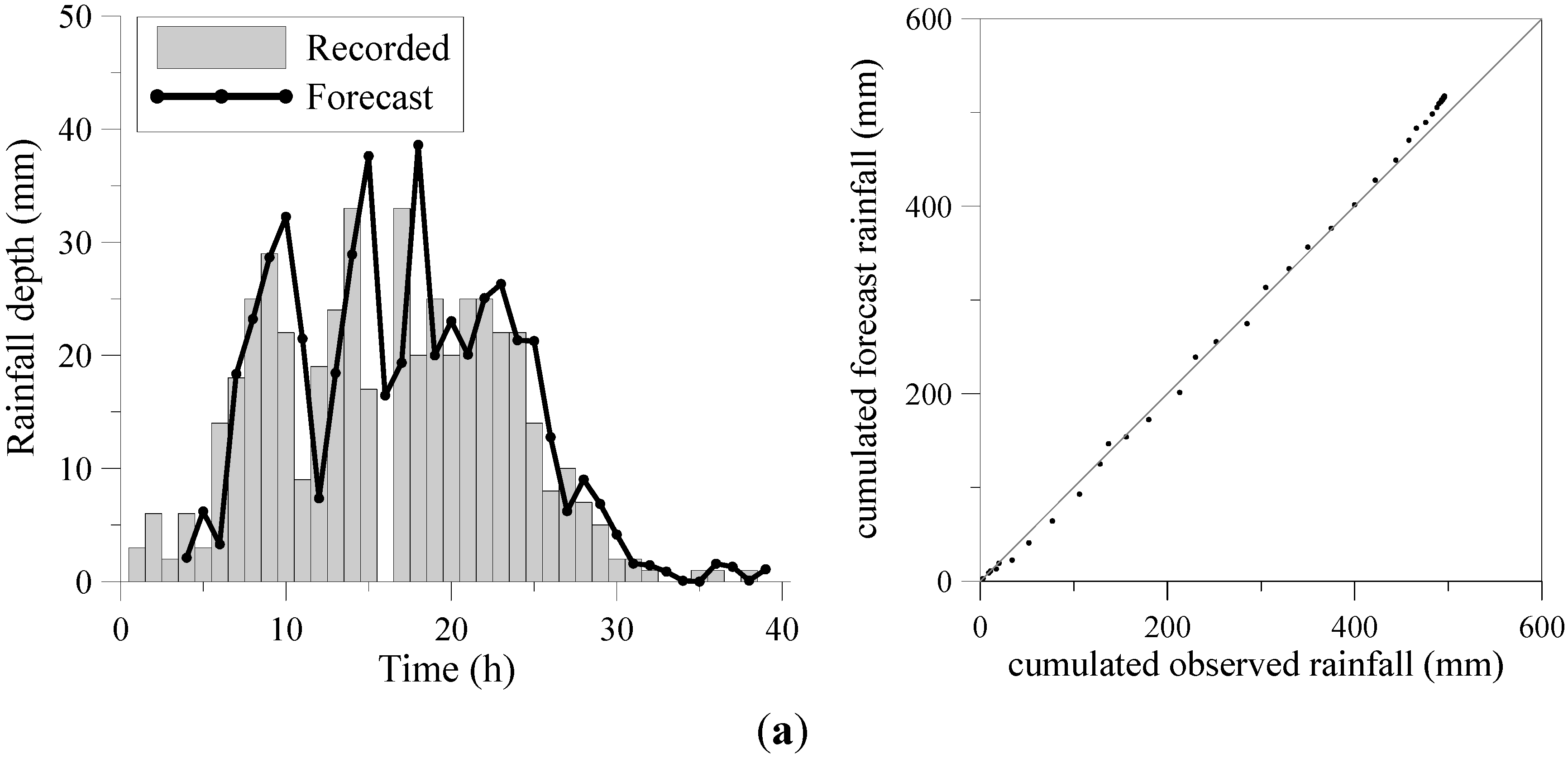
Table 3 and
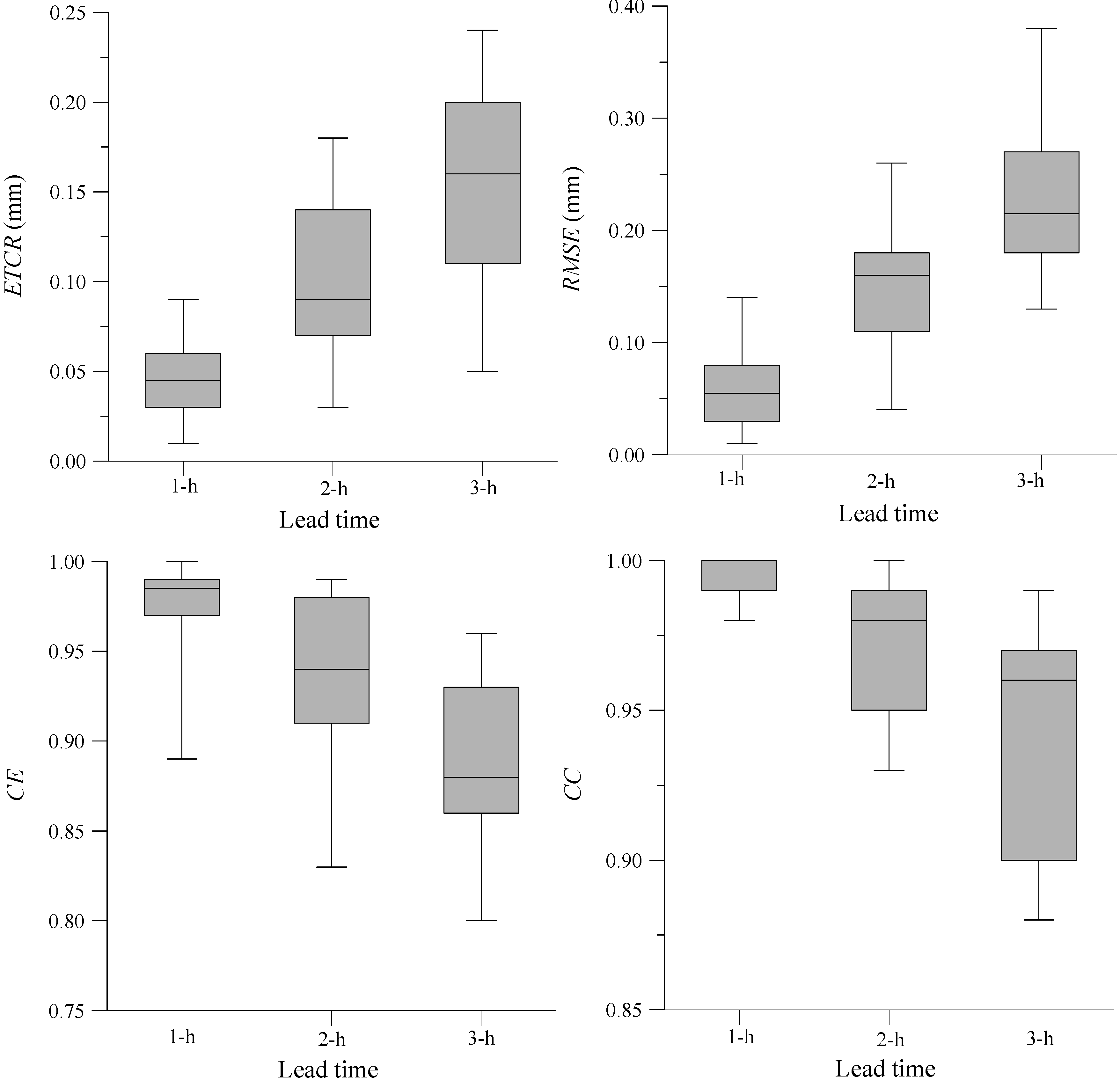
Figure 3 show the performance of the grey rainfall forecasting model for the three watersheds. The
ETCR and RMSE from Equations (9) and (10) represent the quantitative evaluation of the model performance, and
CE from Equation (11) indicates the performance of the model based on cumulative rainfall. The performance of the model was assessed qualitatively based on the value of
CC (Equation (12)) relative to the correlation between the forecast and observed cumulative rainfall. The results showed that
ETCR is less than 0.24,
RMSE is less than 0.38,
CE is greater than 0.85, and
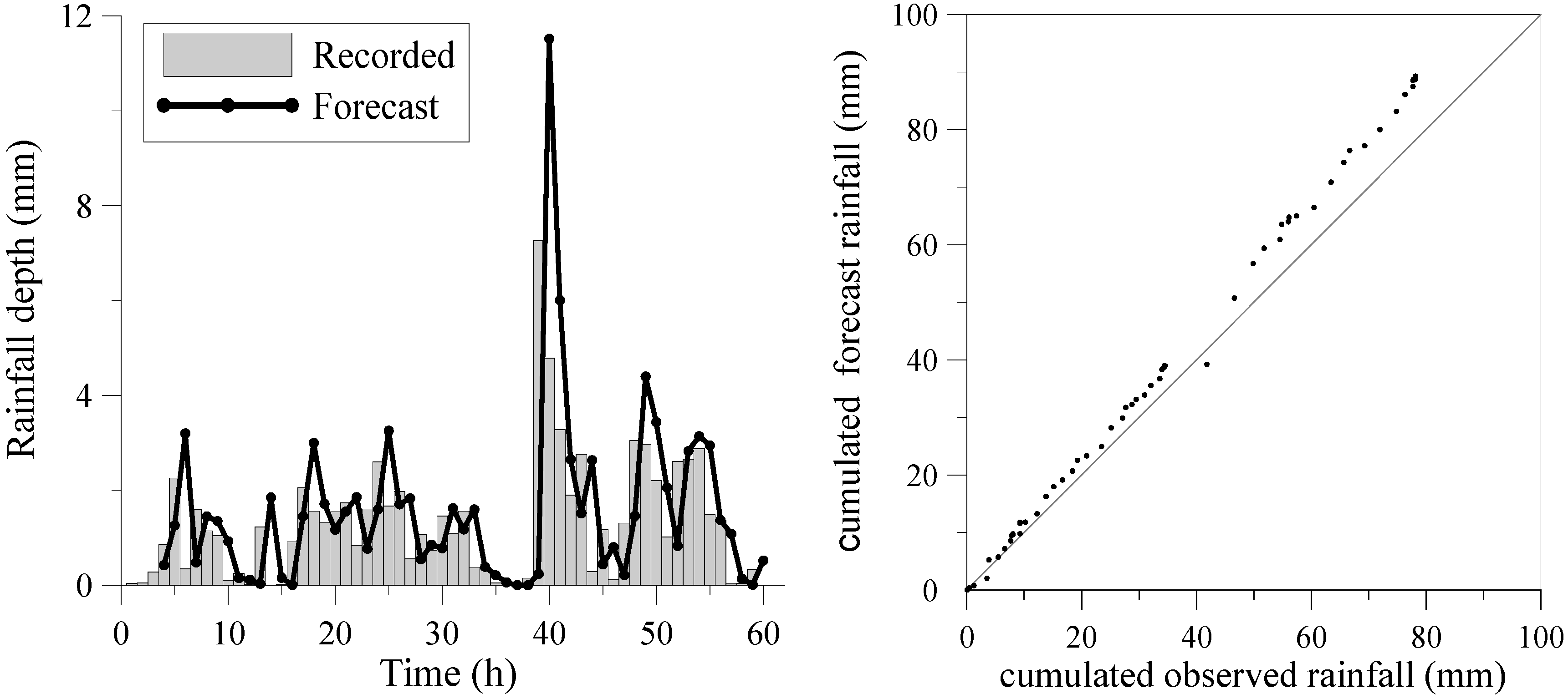
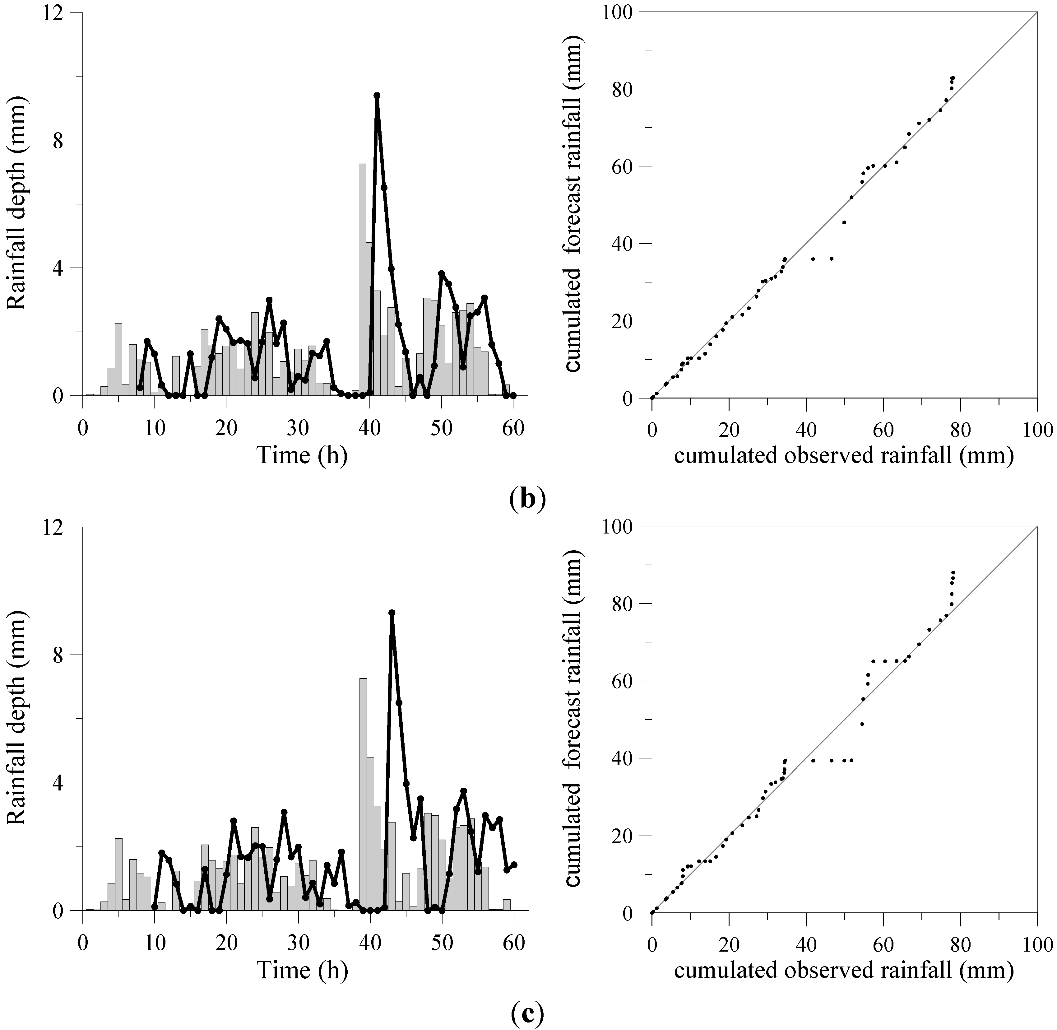
CC is greater than 0.90, indicating that the forecast and recorded hyetographs are in good agreement. The forecast and recorded hyetographs in
Figure 4 and
Figure 5 show the performance of the grey rainfall forecasting model based on lead times ranging from 1 to 3 h. Although the accuracy of the forecast rainfall decreases as the lead time increased, the results indicate that the proposed grey model is suitable for rainfall forecasting.
Table 3.
Results of grey forecast rainfall.
Table 3.
Results of grey forecast rainfall.
| Watershed | Event Date | ETCR | RMSE | CE | CC |
|---|
| 1-h Ahead | 2-h Ahead | 3-h Ahead | 1-h Ahead | 2-h Ahead | 3-h Ahead | 1-h Ahead | 2-h Ahead | 3-h Ahead | 1-h Ahead | 2-h Ahead | 3-h Ahead |
|---|
| Goodwin Creek | 10/07/1989 | 0.03 | 0.18 | 0.22 | 0.03 | 0.08 | 0.17 | 0.99 | 0.98 | 0.92 | 0.99 | 0.95 | 0.88 |
| 02/03/1991 | 0.05 | 0.16 | 0.20 | 0.08 | 0.17 | 0.29 | 0.96 | 0.93 | 0.88 | 0.99 | 0.95 | 0.88 |
| 14/02/1992 | 0.01 | 0.03 | 0.08 | 0.02 | 0.14 | 0.27 | 1.00 | 0.98 | 0.95 | 0.99 | 0.96 | 0.90 |
| 04/08/1995 | 0.06 | 0.11 | 0.16 | 0.04 | 0.17 | 0.24 | 0.97 | 0.90 | 0.87 | 0.99 | 0.98 | 0.92 |
| 29/11/1996 | 0.03 | 0.09 | 0.10 | 0.08 | 0.24 | 0.31 | 0.97 | 0.90 | 0.85 | 0.99 | 0.98 | 0.96 |
| 23/12/1997 | 0.06 | 0.15 | 0.21 | 0.03 | 0.19 | 0.25 | 0.98 | 0.91 | 0.88 | 0.99 | 0.99 | 0.97 |
| 15/02/1998 | 0.04 | 0.07 | 0.16 | 0.06 | 0.11 | 0.19 | 1.00 | 0.94 | 0.88 | 1.00 | 0.96 | 0.97 |
| 13/03/1999 | 0.09 | 0.14 | 0.20 | 0.06 | 0.18 | 0.21 | 0.99 | 0.95 | 0.89 | 1.00 | 0.98 | 0.90 |
| 01/04/2000 | 0.03 | 0.08 | 0.15 | 0.03 | 0.12 | 0.16 | 0.99 | 0.96 | 0.91 | 1.00 | 1.00 | 0.98 |
| 17/01/2001 | 0.07 | 0.11 | 0.19 | 0.07 | 0.11 | 0.16 | 0.98 | 0.91 | 0.88 | 0.98 | 0.94 | 0.91 |
| Heng-Chi and San-Hsia | 17/08/1984 | 0.05 | 0.08 | 0.16 | 0.11 | 0.18 | 0.27 | 0.99 | 0.98 | 0.94 | 1.00 | 0.98 | 0.96 |
| 16/09/1985 | 0.06 | 0.12 | 0.24 | 0.09 | 0.22 | 0.31 | 0.96 | 0.93 | 0.86 | 0.99 | 0.95 | 0.88 |
| 17/09/1986 | 0.01 | 0.03 | 0.05 | 0.05 | 0.18 | 0.21 | 1.00 | 0.98 | 0.95 | 1.00 | 1.00 | 0.99 |
| 27/07/1987 | 0.09 | 0.18 | 0.22 | 0.03 | 0.11 | 0.18 | 0.97 | 0.91 | 0.88 | 0.98 | 0.93 | 0.91 |
| 08/09/1987 | 0.01 | 0.09 | 0.10 | 0.14 | 0.26 | 0.38 | 0.89 | 0.83 | 0.80 | 1.00 | 0.98 | 0.96 |
| 18/08/1990 | 0.03 | 0.09 | 0.12 | 0.08 | 0.17 | 0.24 | 0.95 | 0.85 | 0.81 | 1.00 | 0.99 | 0.97 |
| 05/06/1993 | 0.05 | 0.08 | 0.11 | 0.01 | 0.04 | 0.19 | 1.00 | 0.94 | 0.87 | 0.99 | 0.96 | 0.97 |
| 10/07/1994 | 0.09 | 0.11 | 0.18 | 0.02 | 0.13 | 0.20 | 0.98 | 0.99 | 0.96 | 0.99 | 0.98 | 0.90 |
| 30/07/1996 | 0.04 | 0.07 | 0.11 | 0.05 | 0.15 | 0.22 | 0.99 | 0.95 | 0.83 | 1.00 | 1.00 | 0.98 |
| 31/10/2000 | 0.04 | 0.05 | 0.17 | 0.08 | 0.09 | 0.13 | 0.99 | 0.97 | 0.93 | 1.00 | 1.00 | 0.99 |
| Average | 0.05 | 0.10 | 0.16 | 0.06 | 0.16 | 0.23 | 0.98 | 0.93 | 0.89 | 1.00 | 0.98 | 0.94 |
Figure 3.
Results of evaluated criteria for grey forecast rainfall.
Figure 3.
Results of evaluated criteria for grey forecast rainfall.
Figure 4.
Grey model for rainfall forecasting in Goodwin Creek watershed: (a) 1-h ahead; (b) 2-h ahead; (c) 3-h ahead.
Figure 4.
Grey model for rainfall forecasting in Goodwin Creek watershed: (a) 1-h ahead; (b) 2-h ahead; (c) 3-h ahead.
Figure 5.
Grey model for rainfall forecasting in San-Hsia watershed: (a) 1-h ahead; (b) 2-h ahead; (c) 3-h ahead.
Figure 5.
Grey model for rainfall forecasting in San-Hsia watershed: (a) 1-h ahead; (b) 2-h ahead; (c) 3-h ahead.
3.3. Flow Forecasting
Four sets of tests were performed to evaluate the applicability of the proposed system for real-time flood prediction. The simulation results are detailed shown as follows.
(1) Flow forecasting by using measured rainfall and without flow updating
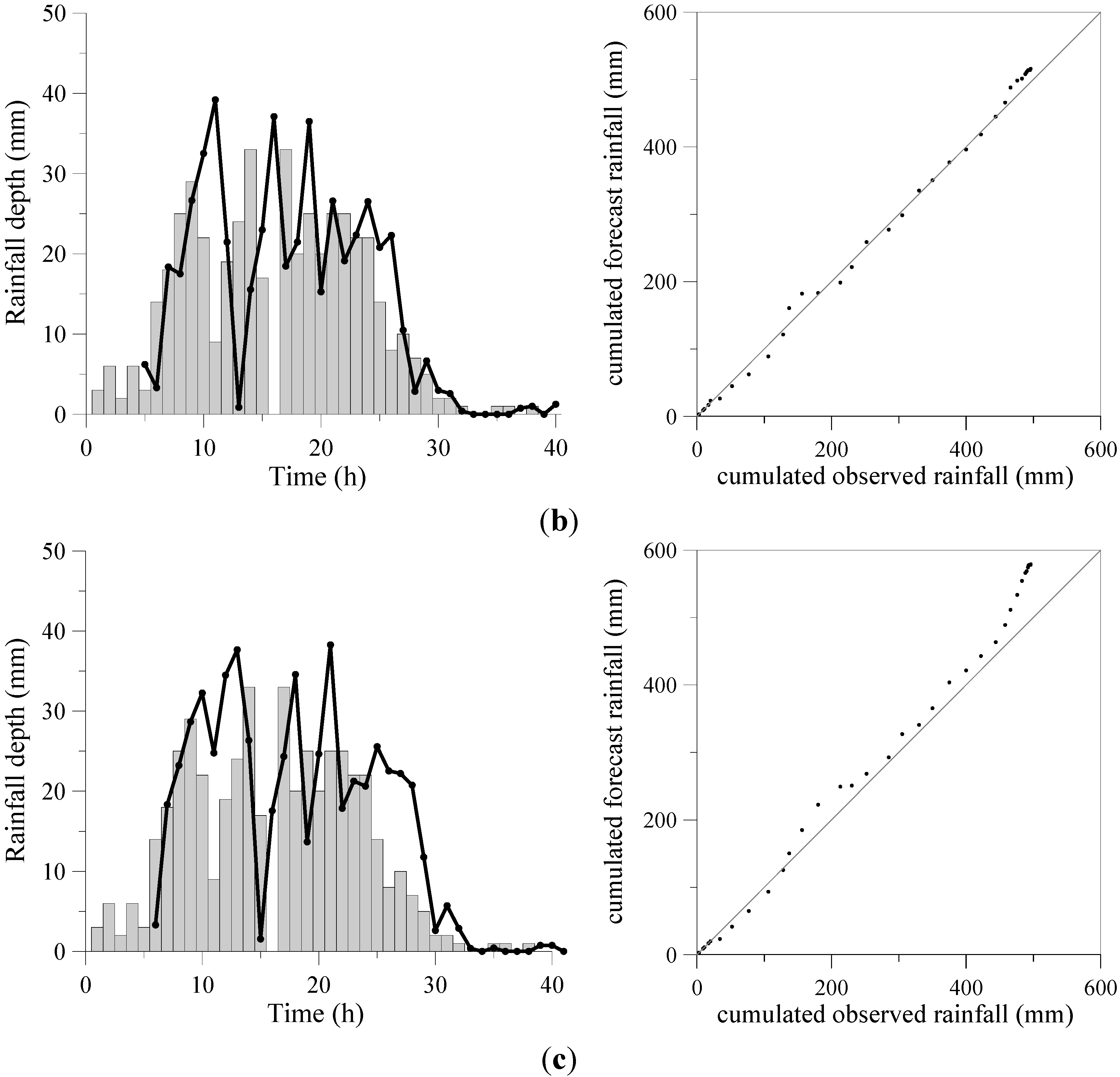
This set of tests was conducted to evaluate the performance of the KW-GIUH model for simulating rainfall-runoff. Observed rainfall data were inputted into the KW-GIUH model and the flow updating algorithm was not used in the simulation.
Figure 6 shows the results of runoff simulations for the Goodwin Creek and San-Hsia watersheds. As shown in
Table 4, the simulated and observed hydrographs are in relatively good agreement in the study watersheds. The
values of the simulated hydrographs for all storm events are greater than 0.82, and most of the
and
are lesser than 10% and 2 h, respectively. The results indicate that the KW-GIUH model is reliable for rainfall-runoff simulation in these two watersheds.
Figure 6a shows that the temporal distributions of the observed rainfall hyetograph and flow hydrograph were inconsistent; specifically, the rainfall peak occurred at 45 h, whereas the flow peak occurred at 57 h. The reason for this inconsistency is unknown. However, this unusual hydrological record could be used to test the effectiveness of the proposed flow updating algorithm.
Figure 6.
Flow forecasting using measured rainfall data and without flow updating in Goodwin Creek and San-Hsia watersheds: (a) Goodwin Creek watershed (STA 01); (b) San-Hsia watershed.
Figure 6.
Flow forecasting using measured rainfall data and without flow updating in Goodwin Creek and San-Hsia watersheds: (a) Goodwin Creek watershed (STA 01); (b) San-Hsia watershed.
Table 4.
Results of flow forecasting using measured rainfall and without flow updating technique.
Table 4.
Results of flow forecasting using measured rainfall and without flow updating technique.
| Watershed | Event Date | CEQ | EQp (%) | ETp (h) |
|---|
| Goodwin (SAT01) | 10/07/1989 | 0.83 | 6.29 | 1 |
| 02/03/1991 | 0.92 | 2.56 | 0 |
| 14/02/1992 | 0.88 | 4.33 | 1 |
| 04/08/1995 | 0.86 | 7.81 | −1 |
| 29/11/1996 | 0.93 | 2.08 | 0 |
| 23/12/1997 | 0.89 | 3.54 | 0 |
| 15/02/1998 | 0.88 | 4.28 | 0 |
| 13/03/1999 | 0.84 | 3.07 | 0 |
| 01/04/2000 | 0.90 | 0.09 | 1 |
| 17/01/2001 | 0.82 | 25.00 | 12 |
| Heng-Chi | 17/08/1984 | 0.92 | 2.00 | −1 |
| 16/09/1985 | 0.88 | 0.24 | −1 |
| 17/09/1986 | 0.85 | 1.82 | 0 |
| 27/07/1987 | 0.86 | 4.16 | 0 |
| 08/09/1987 | 0.92 | 3.46 | 0 |
| 18/08/1990 | 0.85 | 4.52 | −1 |
| 05/06/1993 | 0.97 | 2.01 | −1 |
| 10/07/1994 | 0.86 | 1.25 | −1 |
| 30/07/1996 | 0.94 | 3.54 | −1 |
| 31/10/2000 | 0.95 | 3.01 | −2 |
| San-Hsia | 17/08/1984 | 0.90 | 6.54 | 0 |
| 16/09/1985 | 0.89 | 3.33 | 0 |
| 17/09/1986 | 0.86 | 6.29 | 1 |
| 27/07/1987 | 0.84 | 5.54 | 1 |
| 08/09/1987 | 0.88 | 5.19 | 0 |
| 18/08/1990 | 0.83 | 2.24 | 0 |
| 05/06/1993 | 0.87 | 5.64 | −1 |
| 10/07/1994 | 0.95 | 2.13 | 0 |
| 30/07/1996 | 0.96 | 1.32 | −1 |
| 31/10/2000 | 0.95 | 7.65 | −3 |
| Average | 0.89 | 4.36 | 0.10 |
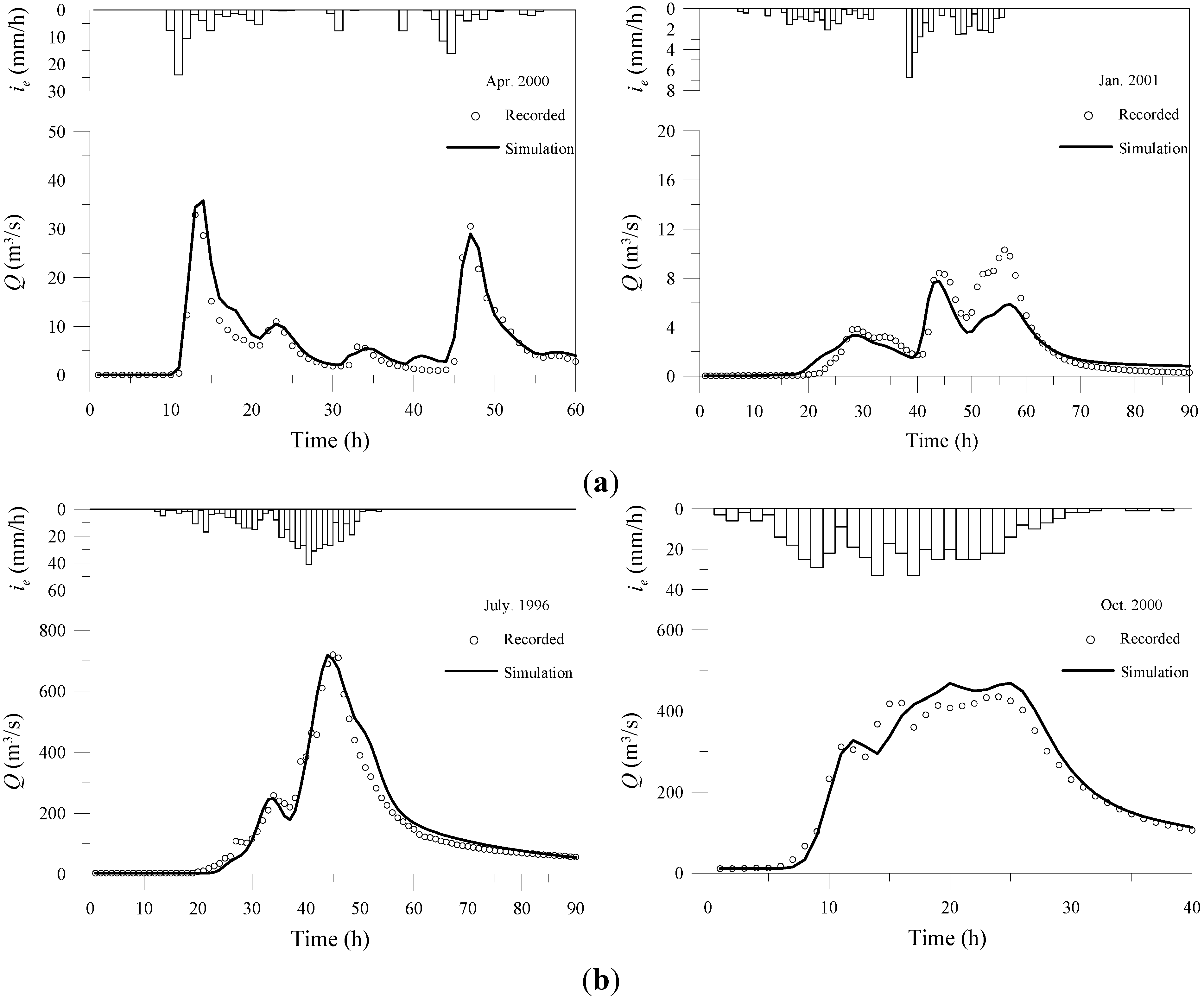
(2) Flow forecasting by using forecast rainfall and without flow updating
For the second set of tests, flow forecasting was performed by inputting the forecast rainfall (obtained from the grey model) into the KW-GIUH model.
Table 5 and
Figure 7 show that the flow forecasting accuracy decreased as the lead time increased from 1 to 3 h. For the
t + 1 forecast, the forecast flow is in good agreement with the observed flow. For the
t + 2 and
t + 3 forecasts, the temporal variation of the flow hydrograph is adequately represented in the simulation although the simulated flow peak is higher than the observed flow peak because the forecast peak rainfall was overestimated in the hyetograph. Regarding the storm event at the Goodwin Creek watershed on 17 January 2001, the results shown in
Figure 7a indicate that the KW-GIUH model forecast the first flow peak accurately. However, the second flow peak is underestimated because of the inconsistency between the rainfall hyetograph and flow hydrograph as mentioned.
Table 5.
Results of flow forecasting using forecast rainfall and without flow updating technique.
Table 5.
Results of flow forecasting using forecast rainfall and without flow updating technique.
| Watershed | Event Date | CEQ | EQp (%) | ETp (h) |
|---|
| 1-h Ahead | 2-h Ahead | 3-h Ahead | 1-h Ahead | 2-h Ahead | 3-h Ahead | 1-h Ahead | 2-h Ahead | 3-h Ahead |
|---|
| Goodwin (SAT01) | 10/07/1989 | 0.82 | 0.49 | 0.31 | 14.41 | 37.91 | 51.18 | 1 | 2 | 3 |
| 02/03/1991 | 0.92 | 0.84 | 0.81 | 9.88 | 27.41 | 39.42 | 1 | 2 | 3 |
| 14/02/1992 | 0.87 | 0.86 | 0.77 | 12.48 | 19.88 | 32.77 | 0 | 1 | 2 |
| 04/08/1995 | 0.86 | 0.83 | 0.77 | 11.82 | 20.43 | 28.91 | 1 | 2 | 3 |
| 29/11/1996 | 0.92 | 0.85 | 0.83 | 8.97 | 14.81 | 17.94 | 0 | 1 | 2 |
| 23/12/1997 | 0.89 | 0.86 | 0.83 | 18.13 | 29.87 | 41.09 | 1 | 1 | 2 |
| 15/02/1998 | 0.87 | 0.81 | 0.69 | 14.30 | 28.99 | 45.17 | 1 | 2 | 3 |
| 13/03/1999 | 0.82 | 0.74 | 0.70 | 7.69 | 12.90 | 18.09 | 0 | 1 | 2 |
| 01/04/2000 | 0.90 | 0.55 | 0.03 | 8.95 | 45.27 | 62.98 | 1 | 2 | 3 |
| 17/01/2001 | 0.82 | 0.81 | 0.80 | 24.75 | 1.27 | 30.97 | 12 | 12 | 12 |
| Heng-Chi | 17/08/1984 | 0.90 | 0.86 | 0.81 | 4.81 | 11.85 | 19.28 | 1 | 2 | 2 |
| 16/09/1985 | 0.87 | 0.81 | 0.74 | 3.29 | 8.74 | 20.32 | 1 | 1 | 2 |
| 17/09/1986 | 0.83 | 0.79 | 0.71 | 10.93 | 24.31 | 31.88 | 1 | 2 | 3 |
| 27/07/1987 | 0.85 | 0.83 | 0.78 | 8.49 | 18.41 | 24.31 | 1 | 2 | 2 |
| 08/09/1987 | 0.92 | 0.90 | 0.86 | 7.96 | 16.19 | 19.22 | 1 | 2 | 2 |
| 18/08/1990 | 0.75 | 0.43 | 0.09 | 14.41 | 19.84 | 31.03 | 1 | 2 | 3 |
| 05/06/1993 | 0.95 | 0.94 | 0.88 | 2.09 | 7.31 | 9.08 | 0 | 1 | 2 |
| 10/07/1994 | 0.85 | 0.81 | 0.70 | 1.09 | 8.54 | 11.72 | 0 | 1 | 1 |
| 30/07/1996 | 0.93 | 0.91 | 0.82 | 9.75 | 14.32 | 18.97 | −1 | 0 | 0 |
| 31/10/2000 | 0.95 | 0.94 | 0.86 | 4.71 | 5.47 | 7.93 | −3 | −2 | −1 |
| San-Hsia | 17/08/1984 | 0.90 | 0.81 | 0.79 | 8.49 | 14.55 | 21.09 | 1 | 2 | 2 |
| 16/09/1985 | 0.88 | 0.80 | 0.74 | 6.39 | 11.52 | 17.92 | 1 | 1 | 2 |
| 17/09/1986 | 0.86 | 0.83 | 0.52 | 9.31 | 18.45 | 37.01 | 1 | 2 | 3 |
| 27/07/1987 | 0.84 | 0.83 | 0.67 | 4.09 | 11.12 | 14.17 | 1 | 2 | 2 |
| 08/09/1987 | 0.87 | 0.81 | 0.63 | 4.41 | 9.18 | 22.97 | 1 | 2 | 2 |
| 18/08/1990 | 0.81 | 0.62 | 0.31 | 6.31 | 11.48 | 18.02 | 1 | 2 | 3 |
| 05/06/1993 | 0.85 | 0.81 | 0.76 | 7.31 | 9.52 | 16.55 | 0 | 1 | 2 |
| 10/07/1994 | 0.95 | 0.91 | 0.85 | 4.86 | 7.59 | 16.31 | 0 | 1 | 1 |
| 30/07/1996 | 0.95 | 0.94 | 0.89 | 1.96 | 4.48 | 12.05 | −1 | 0 | 0 |
| 31/10/2000 | 0.94 | 0.92 | 0.80 | 8.67 | 13.71 | 16.58 | −3 | −2 | −1 |
| Average | 0.88 | 0.80 | 0.69 | 8.69 | 16.18 | 25.16 | 0.73 | 1.60 | 2.23 |
Figure 7.
Flow forecasting using forecast rainfall and without flow updating in Goodwin Creek and San-Hsia watersheds: (a) Goodwin Creek watershed (STA 01); (b) San-Hsia watershed.
Figure 7.
Flow forecasting using forecast rainfall and without flow updating in Goodwin Creek and San-Hsia watersheds: (a) Goodwin Creek watershed (STA 01); (b) San-Hsia watershed.
(3) Flow forecasting by using measured rainfall and flow updating technique
The third set of tests was conducted to evaluate the performance of the KW-GIUH model when the flow updating algorithm was used in the rainfall-runoff simulation, as shown in Equation (18). The measured rainfall at
t + 1,
t + 2, and
t + 3 was inputted into the KW-GIUH model.
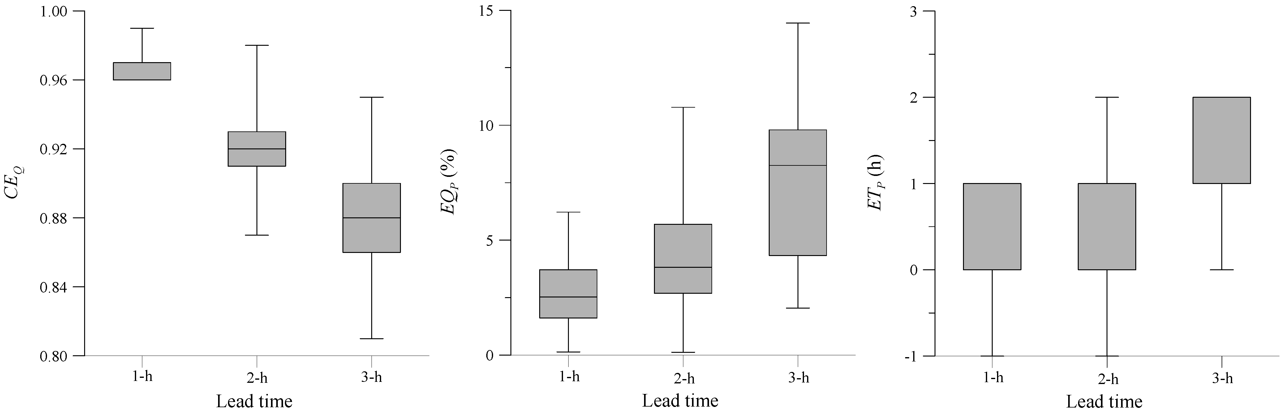
Table 6 and
Figure 8 show the simulation results, which were evaluated based on the coefficient of efficiency
, error of peak discharge
, and error of time to peak discharge
. When the value
is approximately one and
and
are approximately zero, good agreement between the recorded and simulated hydrographs is anticipated. The results in
Figure 8 show that the
values are higher than 0.96, the mean
is 2.73%, and the mean
is 0.17 h for the
t + 1 simulation. For the
t + 2 simulation, the
values are higher than 0.87, the mean
is 4.40%, and the mean
is 0.67 h. Finally, for the
t + 3 simulation, the
values are higher than 0.81, the mean
is 7.92%, and the mean
is 1.23 h.
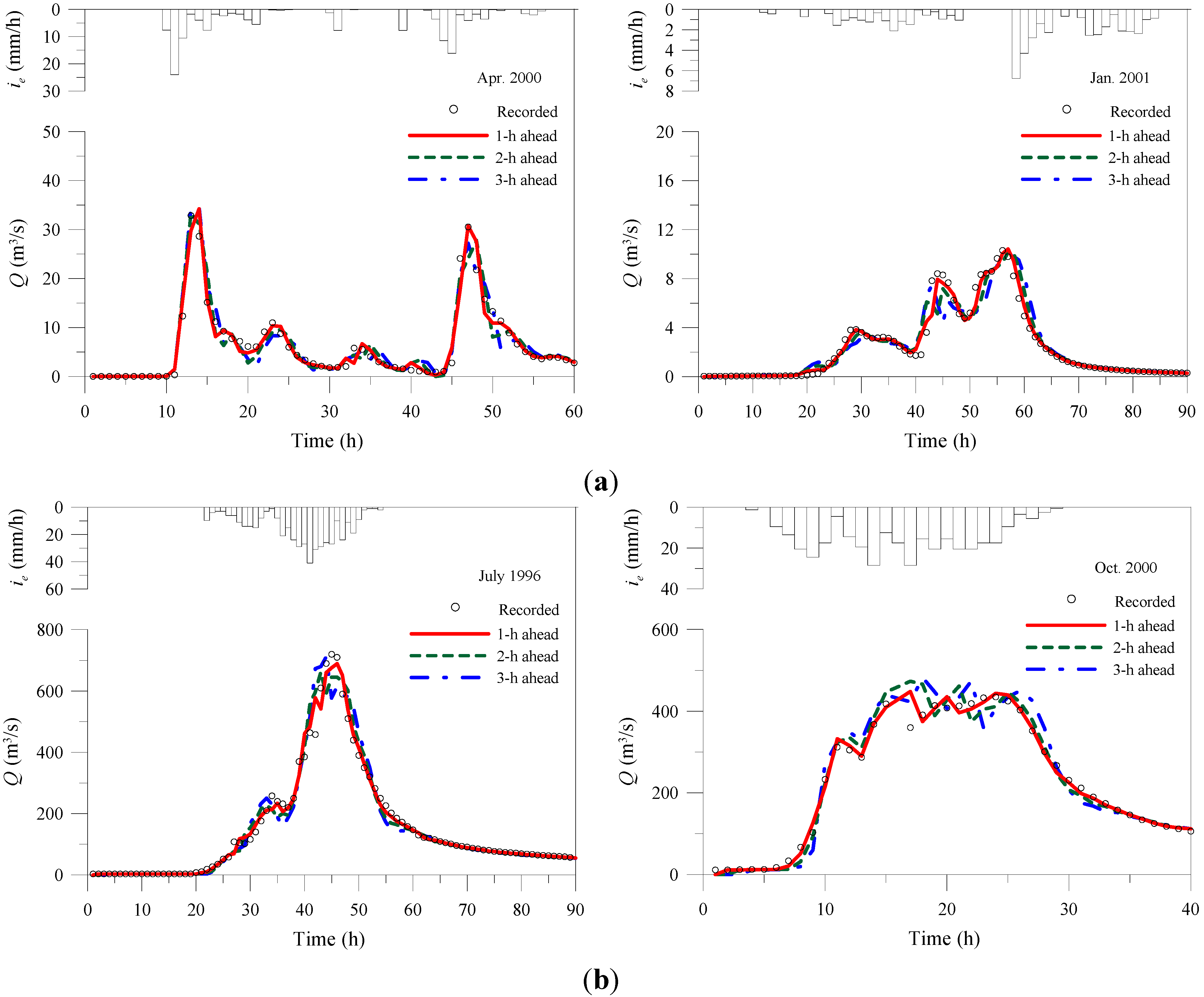
Figure 9 shows that the forecast and recorded hydrographs are in good agreement for all storm events in this test, indicating that the proposed flow updating algorithm combined with the KW-GIUH model simulated the watershed runoff more accurately than do the KW-GIUH model alone. Moreover, regarding the storm event at the Goodwin Creek watershed on 17 January 2001, the flow hydrographs in
Figure 7a and
Figure 9a show that the second peak was accurately forecasted when the flow updating algorithm is used, despite the recorded flow peak appearing to be unreasonable. The results show that using a purely deterministic approach to simulate watershed rainfall runoff is difficult without the assistance of a real-time adaptive algorithm.
Table 6.
Results of flow forecasting using measured rainfall and flow updating technique.
Table 6.
Results of flow forecasting using measured rainfall and flow updating technique.
| Watershed | Event Date | CEQ | EQp (%) | ETp (h) |
|---|
| 1-h Update | 2-h Update | 3-h Update | 1-h Update | 2-h Update | 3-h Update | 1-h Update | 2-h Update | 3-h Update |
|---|
| Goodwin (SAT01) | 10/07/1989 | 0.97 | 0.93 | 0.89 | 2.54 | 5.77 | 8.43 | 1 | 1 | 1 |
| 02/03/1991 | 0.98 | 0.94 | 0.90 | 0.14 | 3.43 | 4.95 | 1 | 1 | 2 |
| 14/02/1992 | 0.96 | 0.91 | 0.84 | 3.83 | 5.46 | 5.57 | 0 | 0 | 1 |
| 04/08/1995 | 0.96 | 0.92 | 0.83 | 2.53 | 4.59 | 7.33 | 0 | 0 | 1 |
| 29/11/1996 | 0.96 | 0.91 | 0.85 | 3.64 | 4.22 | 8.36 | 1 | 2 | 2 |
| 23/12/1997 | 0.97 | 0.92 | 0.85 | 4.81 | 5.65 | 8.78 | −1 | 0 | 1 |
| 15/02/1998 | 0.96 | 0.92 | 0.86 | 0.19 | 3.19 | 3.97 | −1 | −1 | 0 |
| 13/03/1999 | 0.96 | 0.91 | 0.83 | 3.71 | 0.13 | 9.80 | 0 | 1 | 1 |
| 01/04/2000 | 0.97 | 0.93 | 0.85 | 1.94 | 0.97 | 8.11 | −1 | −1 | 0 |
| 17/01/2001 | 0.97 | 0.87 | 0.81 | 0.84 | 0.53 | 2.05 | 1 | 1 | 1 |
| Heng-Chi | 17/08/1984 | 0.96 | 0.92 | 0.88 | 4.75 | 5.69 | 10.54 | 0 | 0 | 1 |
| 16/09/1985 | 0.97 | 0.93 | 0.89 | 4.55 | 6.29 | 14.12 | 0 | 0 | 1 |
| 17/09/1986 | 0.97 | 0.92 | 0.90 | 2.30 | 1.89 | 4.92 | 0 | 1 | 2 |
| 27/07/1987 | 0.96 | 0.91 | 0.88 | 0.76 | 2.69 | 5.50 | 0 | 1 | 1 |
| 08/09/1987 | 0.96 | 0.92 | 0.89 | 1.62 | 5.86 | 8.80 | 1 | 2 | 2 |
| 18/08/1990 | 0.97 | 0.93 | 0.91 | 0.50 | 3.40 | 4.14 | −1 | 0 | 0 |
| 05/06/1993 | 0.98 | 0.93 | 0.91 | 2.75 | 0.68 | 8.15 | 1 | 2 | 2 |
| 10/07/1994 | 0.97 | 0.93 | 0.90 | 3.03 | 4.42 | 9.09 | 1 | 1 | 2 |
| 30/07/1996 | 0.96 | 0.91 | 0.89 | 3.16 | 2.19 | 2.09 | 0 | 0 | 1 |
| 31/10/2000 | 0.98 | 0.93 | 0.91 | 3.17 | 10.78 | 14.44 | 0 | 1 | 1 |
| San-Hsia | 17/08/1984 | 0.96 | 0.92 | 0.87 | 2.95 | 5.69 | 12.86 | 1 | 1 | 2 |
| 16/09/1985 | 0.96 | 0.91 | 0.88 | 1.21 | 8.33 | 13.23 | 0 | 1 | 1 |
| 17/09/1986 | 0.97 | 0.92 | 0.89 | 1.53 | 1.64 | 3.23 | 0 | 1 | 1 |
| 27/07/1987 | 0.97 | 0.92 | 0.88 | 3.76 | 3.24 | 4.18 | 0 | 0 | 1 |
| 08/09/1987 | 0.97 | 0.91 | 0.86 | 1.64 | 6.24 | 10.8 | 0 | 1 | 2 |
| 18/08/1990 | 0.96 | 0.91 | 0.88 | 1.69 | 3.23 | 3.15 | 0 | 0 | 1 |
| 05/06/1993 | 0.97 | 0.94 | 0.91 | 2.42 | 4.89 | 9.33 | 1 | 2 | 2 |
| 10/07/1994 | 0.96 | 0.91 | 0.88 | 1.72 | 3.09 | 11.56 | 0 | 0 | 1 |
| 30/07/1996 | 0.98 | 0.98 | 0.93 | 3.84 | 3.28 | 4.34 | −1 | 0 | 1 |
| 31/10/2000 | 0.99 | 0.96 | 0.95 | 6.22 | 7.35 | 9.42 | 1 | 2 | 2 |
| Average | 0.97 | 0.92 | 0.88 | 2.73 | 4.40 | 7.92 | 0.17 | 0.67 | 1.23 |
Figure 8.
Results of evaluated criteria for flow forecasting using measured rainfall and flow updating technique.
Figure 8.
Results of evaluated criteria for flow forecasting using measured rainfall and flow updating technique.
Figure 9.
Flow forecasting using measured rainfall and flow updating algorithm in Goodwin Creek and San-Hsia watersheds: (a) Goodwin Creek watershed (STA 01); (b) San-Hsia watershed.
Figure 9.
Flow forecasting using measured rainfall and flow updating algorithm in Goodwin Creek and San-Hsia watersheds: (a) Goodwin Creek watershed (STA 01); (b) San-Hsia watershed.
(4) Flow forecasting by using forecast rainfall and flow updating algorithm
The final set tests was conducted to confirm the performance of the proposed flood forecasting system. The forecast rainfall is generated by using the grey model, and the flow updating algorithm is included in the runoff simulation by using the KW-GIUH model to improve the forecasting accuracy.
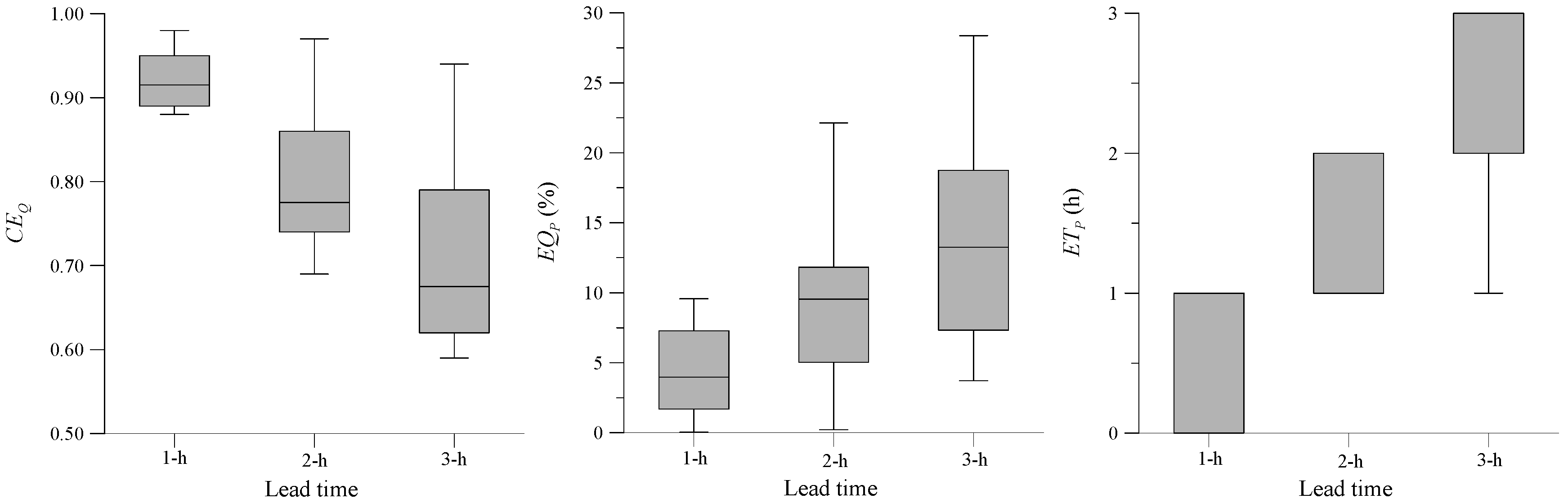
Table 7 and
Figure 10 show that the mean
(
) values of the
t + 1,
t + 2, and
t + 3 forecasts are 0.92 (4.50%), 0.80 (9.12%), and 0.72 (13.57%). The mean
values of the
t + 1,
t + 2, and
t + 3 forecasts are 0.70 h, 1.47 h, and 2.13 h, respectively. The results of the storm event simulations in
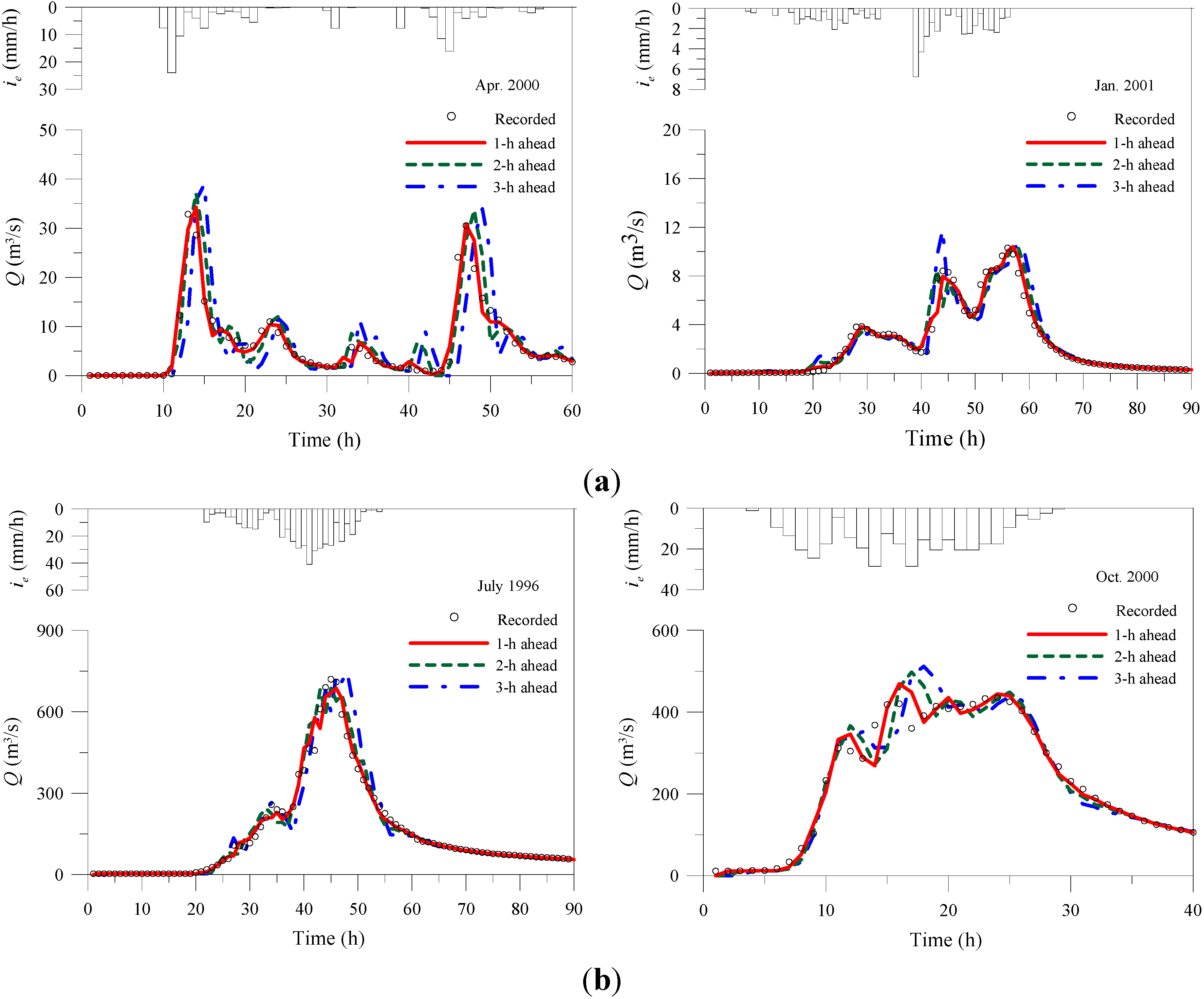
Figure 11 shows that the recorded and simulated hydrographs are in good agreement for all the three watersheds under various geoclimate conditions, even as the lead time increases from 1 to 3 h.
Table 7.
Results of flow forecasting using forecast rainfall and flow updating technique.
Table 7.
Results of flow forecasting using forecast rainfall and flow updating technique.
| Watershed | Event Date | CEQ | EQp (%) | ETp (h) |
|---|
| 1-h Ahead | 2-h Ahead | 3-h Ahead | 1-h Ahead | 2-h Ahead | 3-h Ahead | 1-h Ahead | 2-h Ahead | 3-h Ahead |
|---|
| Goodwin (SAT01) | 10/07/1989 | 0.94 | 0.82 | 0.80 | 3.81 | 11.21 | 13.91 | 1 | 1 | 2 |
| 02/03/1991 | 0.95 | 0.87 | 0.77 | 1.00 | 3.60 | 7.33 | 1 | 1 | 2 |
| 14/02/1992 | 0.89 | 0.69 | 0.66 | 4.22 | 1.89 | 4.04 | 1 | 2 | 2 |
| 04/08/1995 | 0.88 | 0.70 | 0.69 | 1.01 | 8.67 | 12.59 | 1 | 2 | 3 |
| 29/11/1996 | 0.89 | 0.86 | 0.81 | 3.64 | 9.45 | 16.24 | 1 | 1 | 2 |
| 23/12/1997 | 0.91 | 0.69 | 0.65 | 7.28 | 8.15 | 14.89 | 0 | 1 | 2 |
| 15/02/1998 | 0.93 | 0.85 | 0.79 | 9.56 | 10.69 | 11.28 | 0 | 1 | 2 |
| 13/03/1999 | 0.91 | 0.79 | 0.78 | 3.70 | 8.91 | 7.28 | 0 | 1 | 1 |
| 01/04/2000 | 0.95 | 0.72 | 0.61 | 4.13 | 12.34 | 18.75 | 1 | 2 | 3 |
| 17/01/2001 | 0.97 | 0.94 | 0.91 | 1.07 | 0.39 | 4.20 | 0 | 1 | 1 |
| Heng-Chi | 17/08/1984 | 0.95 | 0.76 | 0.62 | 8.42 | 11.21 | 3.71 | 1 | 1 | 2 |
| 16/09/1985 | 0.89 | 0.71 | 0.61 | 4.88 | 13.77 | 5.66 | 1 | 1 | 2 |
| 17/09/1986 | 0.90 | 0.84 | 0.79 | 1.52 | 8.15 | 19.10 | 1 | 2 | 3 |
| 27/07/1987 | 0.96 | 0.76 | 0.61 | 6.79 | 9.97 | 11.52 | 1 | 2 | 2 |
| 08/09/1987 | 0.89 | 0.75 | 0.62 | 0.04 | 7.44 | 16.60 | 1 | 2 | 3 |
| 18/08/1990 | 0.91 | 0.78 | 0.66 | 3.21 | 0.22 | 9.67 | 0 | 1 | 1 |
| 05/06/1993 | 0.88 | 0.77 | 0.61 | 7.93 | 12.73 | 19.02 | 1 | 2 | 3 |
| 10/07/1994 | 0.92 | 0.74 | 0.64 | 3.28 | 11.82 | 23.11 | 1 | 1 | 2 |
| 30/07/1996 | 0.96 | 0.90 | 0.83 | 1.70 | 3.62 | 6.61 | 1 | 2 | 2 |
| 31/10/2000 | 0.95 | 0.89 | 0.82 | 3.68 | 5.03 | 10.02 | 1 | 2 | 2 |
| San-Hsia | 17/08/1984 | 0.93 | 0.76 | 0.63 | 9.31 | 11.59 | 17.42 | 1 | 2 | 3 |
| 16/09/1985 | 0.89 | 0.74 | 0.61 | 5.81 | 14.60 | 19.88 | 1 | 2 | 2 |
| 17/09/1986 | 0.91 | 0.91 | 0.78 | 8.44 | 18.00 | 22.30 | 0 | 1 | 2 |
| 27/07/1987 | 0.89 | 0.72 | 0.59 | 7.32 | 11.52 | 15.39 | 1 | 2 | 3 |
| 08/09/1987 | 0.96 | 0.83 | 0.74 | 1.75 | 5.47 | 14.50 | 0 | 1 | 1 |
| 18/08/1990 | 0.91 | 0.75 | 0.65 | 1.68 | 3.13 | 9.50 | 1 | 2 | 2 |
| 05/06/1993 | 0.88 | 0.71 | 0.63 | 6.03 | 22.14 | 27.56 | 1 | 2 | 3 |
| 10/07/1994 | 0.92 | 0.78 | 0.69 | 1.32 | 13.36 | 28.36 | 0 | 1 | 2 |
| 30/07/1996 | 0.98 | 0.97 | 0.92 | 4.60 | 4.83 | 5.03 | 1 | 1 | 2 |
| 31/10/2000 | 0.98 | 0.95 | 0.94 | 7.75 | 9.65 | 11.62 | 0 | 1 | 2 |
| Average | 0.92 | 0.80 | 0.72 | 4.50 | 9.12 | 13.57 | 0.70 | 1.47 | 2.13 |
Figure 10.
Results of evaluated criteria for flow forecasting using forecast rainfall and flow updating technique.
Figure 10.
Results of evaluated criteria for flow forecasting using forecast rainfall and flow updating technique.
Figure 11.
Flow forecasting using forecast rainfall and flow updating algorithm in Goodwin Creek and San-Hsia watersheds: (a) Goodwin Creek watershed (STA 01); (b) San-Hsia watershed.
Figure 11.
Flow forecasting using forecast rainfall and flow updating algorithm in Goodwin Creek and San-Hsia watersheds: (a) Goodwin Creek watershed (STA 01); (b) San-Hsia watershed.


