Parameter Automatic Calibration Approach for Neural-Network-Based Cyclonic Precipitation Forecast Models

Abstract

This paper presents artificial neural network (ANN)-based models for forecasting precipitation, in which the training parameters are adjusted using a parameter automatic calibration (PAC) approach. A classical ANN-based model, the multilayer perceptron (MLP) neural network, was used to verify the utility of the proposed ANN–PAC approach. The MLP-based ANN used the learning rate, momentum, and number of neurons in the hidden layer as its major parameters. The Dawu gauge station in Taitung, Taiwan, was the study site, and observed typhoon characteristics and ground weather data were the study data. The traditional multiple linear regression model was selected as the benchmark for comparing the accuracy of the ANN–PAC model. In addition, two MLP ANN models based on a trial-and-error calibration method, ANN–TRI1 and ANN–TRI2, were realized by manually tuning the parameters. We found the results yielded by the ANN–PAC model were more reliable than those yielded by the ANN–TRI1, ANN–TRI2, and traditional regression models. In addition, the computing efficiency of the ANN–PAC model decreased with an increase in the number of increments within the parameter ranges because of the considerably increased computational time, whereas the prediction errors decreased because of the model’s increased capability of identifying optimal solutions.

1. Introduction

Taiwan is a long and narrow island located between Japan and the Philippines in the Western Pacific and has an area of 35,981 km²; the Central Mountain Range runs from north to south, and the Tropic of Cancer passes through the south. On average, approximately 80 tropical cyclones, also known as typhoons, form annually worldwide, of which approximately 30 form in the western North Pacific. Most typhoons in Taiwan form between May and November, and, on average, 3.9 typhoons affect Taiwan each year. As soon as a typhoon strikes, it often causes continuous torrential rainfall, leading to severe flooding, landslides, and debris flow [1]. Therefore, an effective and quantitative precipitation forecast model for typhoon periods is necessary.

The concept of artificial neurons was first introduced in 1943 [2]. In the late 1980s, research on artificial neural network (ANN) applications advanced after the introduction of backpropagation training algorithms for feedforward ANNs [3]. ANNs, which simulate the biological nervous system and brain activity, have become the preferred forecasting approach in hydrology and hydrometeorology (e.g., [4,5,6,7,8,9,10,11,12,13,14,15,16,17,18,19]). ANNs are advantageous because feedforward networks are universal approximators capable of learning continuous functions with any desired degree of accuracy. Most ANN models have several parameters that users can adjust for realizing different scenarios and objectives, and the results produced by such models are typically distinct, which renders identifying the unique optimal solution difficult [20].

To realize a model that accurately represents the system being modeled, the model parameters must be determined using known system inputs and responses; the process of determining the optimal value of these parameters is termed “calibration.” Traditionally, ANN-based models are calibrated using trial-and-error approaches [21]. Maier and Dandy [22] reviewed numerous ANNs and reported that several heuristic calibration approaches have been proposed in which the models dynamically adapt the learning rate and momentum value as training progresses. The majority of these approaches are based on the principle of increasing the step size taken in weight space when successive weight updates reduce the error (or when the steps are in the same direction) and reducing the step size when the error increases in consecutive iterations (or when the steps are in opposite directions) (e.g., [23,24,25,26,27,28,29,30,31,32,33]). For calibrating hidden neurons, Sheela and Deepa [34] reviewed various methods for fixing the number of hidden neurons in ANNs and reported that randomly selecting the number of hidden neurons can result in overfitting or underfitting. Empirical studies have shown that optimizing these parameters is highly problem-dependent [35,36].

Trial-and-error calibration approaches are easy to comprehend but the results are not always satisfactory unless the modeler is experienced. As indicated by Cai et al. [20], the parameters are typically separately adjusted during trial-and-error calibration. The adjustment of a parameter is stopped when no further improvement is made in the goodness-of-fit, and the same process is applied to optimize each parameter without considering the effects of the other parameters. Although this method is simple and widely accepted, it can produce unsatisfactory and suboptimal results.

This paper presents the development of ANN-based models for forecasting precipitation in which the training parameters are adjusted using a parameter automatic calibration (PAC) approach. A classical ANN-based multilayer perceptron (MLP) neural network was used to demonstrate the utility of the proposed PAC approach. MLP neural networks are extensively used to model an unknown system with observable inputs and outputs, which is similar to synthesizing an approximation of a set of multidimensional functions, and are widely employed because of their simplicity, flexibility, and ease of use. The developed methodology was used to construct precipitation forecasting models for the Dawu gauge station in Taitung, Taiwan. The performance of the ANN–PAC model in the analysis of historical typhoon events was compared with those of various ANN-based models that employ trial-and-error calibration and traditional linear multiple regressions.

2. Methodology

The MLP ANN is briefly introduced before the methodology of the ANN–PAC algorithm is presented.

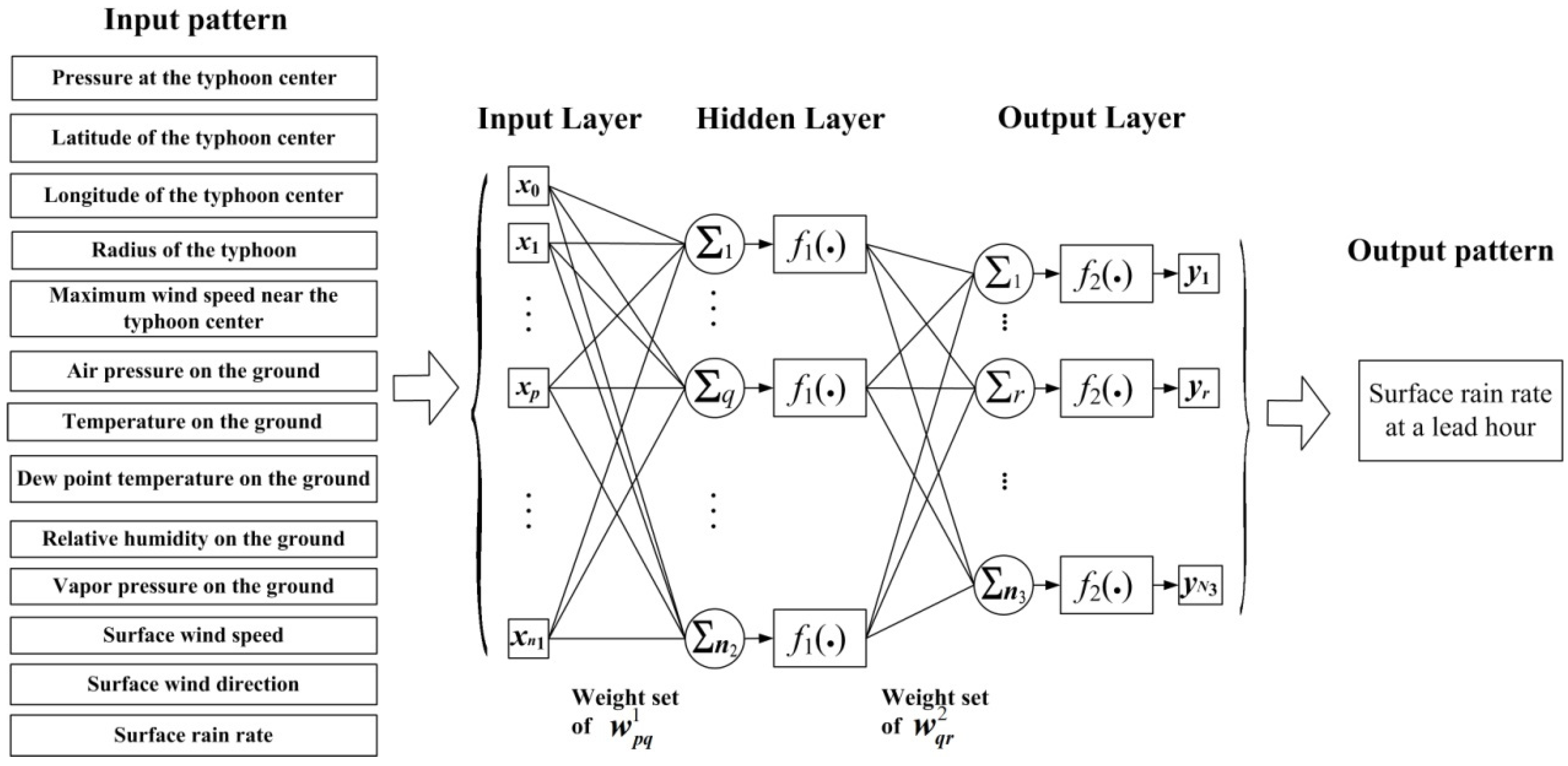
2.1. Sketch of MLP ANN

MLPs are feedforward neural networks trained using a standard backpropagation algorithm. They are supervised networks and the desired response must be trained [37]. MLP networks often consist of an input layer, one or more nonlinear hidden layers, and a linear output layer. Each layer may contain one or more nonlinear processing units called neurons or nodes [38]. Figure 1 is a scheme of a typical MLP network featuring three layers: input, hidden, and output layers. Mathematically, a three-layer MLP comprising n₁ input nodes, n₂ hidden nodes, and n₃ output nodes, is expressed as:

$$y_r=f_2\left({\displaystyle \sum _{q=0}^{n_2}{w}_{qr}^2\cdot f_1\left({\displaystyle \sum _{p=0}^{n_1}{w}_{pq}^1\cdot x_p}\right)}\right)\begin{array}{}\end{array}\begin{array}{}\end{array}r\in [1,n_3]$$

(1)

where p, q, and r are the indices of the input, hidden, and output nodes, respectively; $x_p$ is the input node of the input layer, $w_{pq}^1$ is the weight set connecting the input and hidden layers, $w_{qr}^2$ is the weight set connecting the hidden and output layers, $y_r$ denotes the network outputs, f₁(g) is the activity function of the hidden layer, and f₂(g) is the activity function of the output layer.

In a MLP network, the output is generated by passing signals from the input layer to the output layer through the hidden layer. When constructing an MLP structure, the number of neurons in the hidden layer is not constant and must be optimized depending on the characteristics of the application [39]. The inputs to a perceptron are weighted, summed over the inputs, translated, and passed through an activation function. The frequently used activity functions include linear, sigmoidal, and hyperbolic tangents [40]. As the training progresses, the weights are updated systematically using the backpropagation algorithm and the network output is compared with the target output. The learning acquired by the network is stored in its weights in a distributed manner. An MLP comprises major parameters, namely the learning rate, momentum, and number of nodes in the hidden layer. These parameters are typically set on the basis of experience or are adjusted one parameter at a time and their effect on the model observed [20].

Figure 1. Architecture of the three-layer multilayer perceptron (MLP) neural network.

Figure 1. Architecture of the three-layer multilayer perceptron (MLP) neural network.

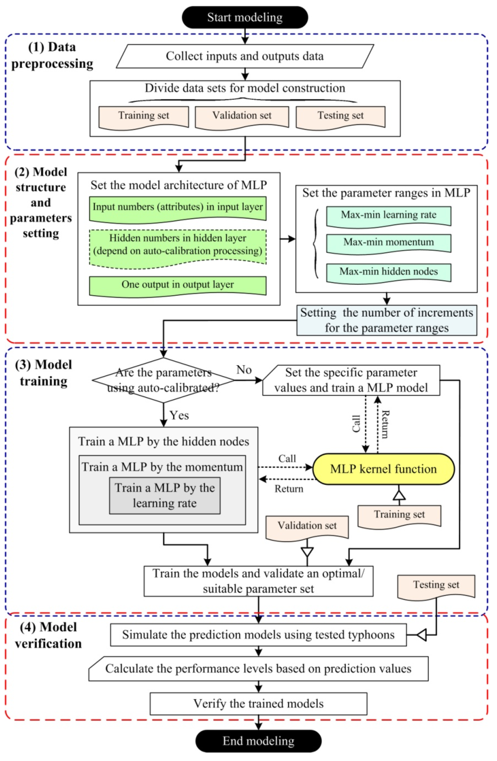
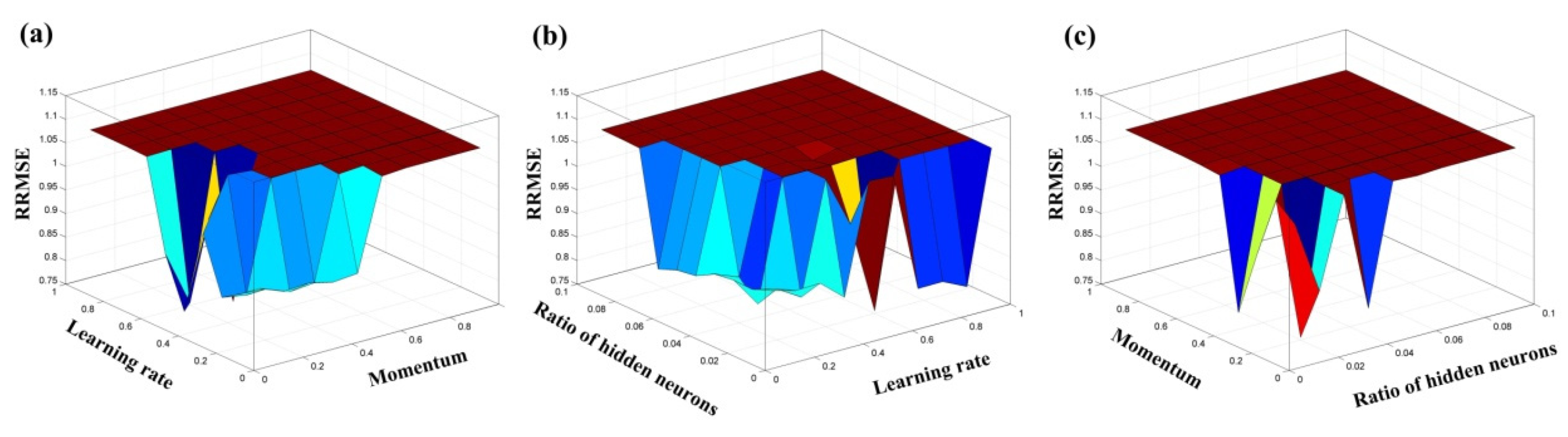
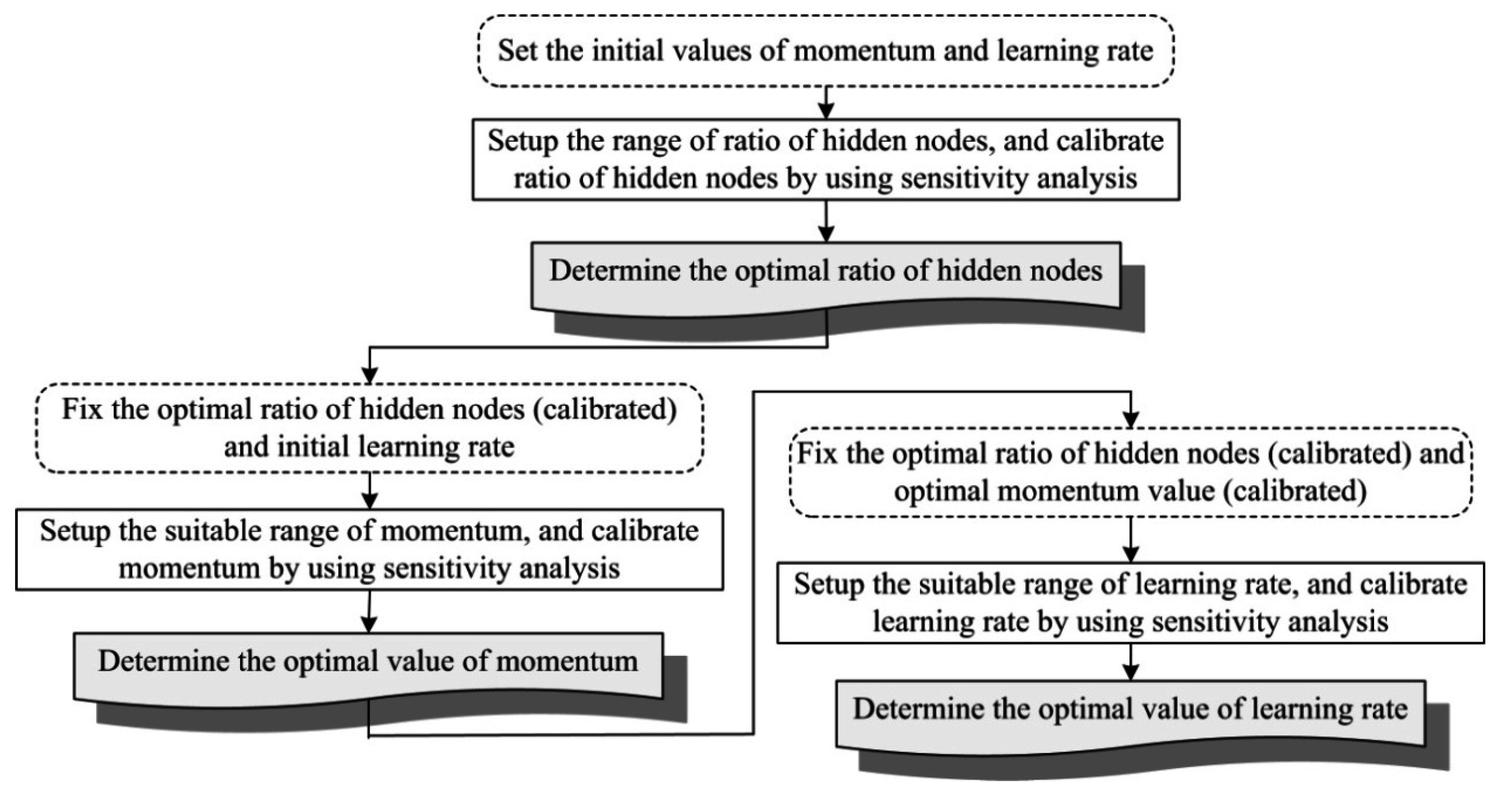
2.2. Proposed ANN–PAC Model

In this section, a methodology is presented for an ANN–PAC approach in forecasting precipitation during typhoons. Figure 2 illustrates the flowchart of the proposed method, and each step is described as follows.

Phase 1, Data Preprocessing: The collected data contain typhoon characteristics and ground weather data (Section 3.1). Because a traditional training–validation–test procedure is adopted for the optimization of an ANN model, the collected data are classified into training, validation, and testing subsets. The training set is used to build model structures and adjust the connected weights of the constructed models. The validation set is used to validate an optimal parameter set, and the testing set is used to evaluate the performance of the constructed models and confirm their generalizability.

Phase 2, Model Structure and Parameters Setting: The model architecture of the MLP model is fixed, including the number of inputs (attributes) in the input layer, the number of neurons in the hidden layer (considered a decision variable in this study and optimized through automatic calibration), and the output in the output layer. Subsequently, the ranges of three critical parameters in the MLP network—the learning rate, momentum, and number of neurons in the hidden layer—are set. Finally, the number of increments between maximal and minimal parameter values is fixed.

Phase 3, Model Training: First, a decision condition selects whether the model parameters are calibrated automatically. If “yes”, the modeling process proceeds in the three-loop training structure by using the parameter values designed in Phase 2; if “no”, the parameter values are set manually (i.e., trial-and-error calibration). The training process is initiated using a training set; the MLP kernel function is repeatedly called and the outputs returned for training the model. The trained models are validated using a validation set. Then, the optimal trained model and their parameter set are identified.

Phase 4, Model Verification: The tested typhoons (i.e., a testing set) are simulated using the optimal trained model, and the forecast results are evaluated according to the performance measures.

In Phase 3, when training the ANN model we performed an early stopping procedure to avoid overfitting caused by an overly close reconstruction of the data in the training set. The stopping procedure is briefly described as follows: first, the backpropagation algorithm is applied on a training set. The performance of the obtained input–output map is then iteratively validated in a validation set. The iteration process is stopped when the performance in the validation set begins to decrease, even if the performance in the training set continues to increase under the desired threshold. Detailed descriptions were provided by Pasini [41] and Prechelt and Orr [42].

Figure 2. Determining artificial neural network (ANN)-based MLP parameters using an automatic calibration approach.

Figure 2. Determining artificial neural network (ANN)-based MLP parameters using an automatic calibration approach.

3. Experiment

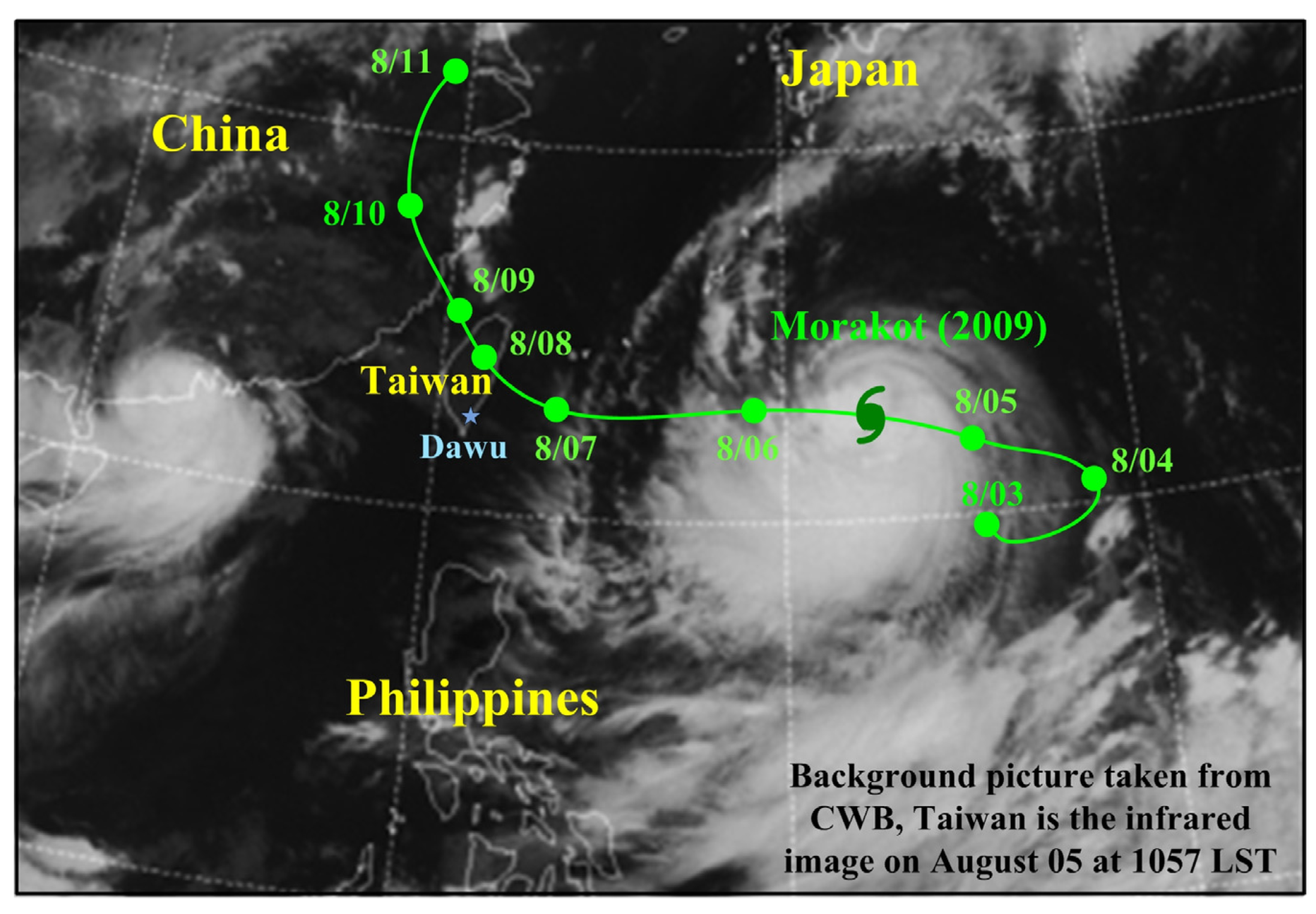
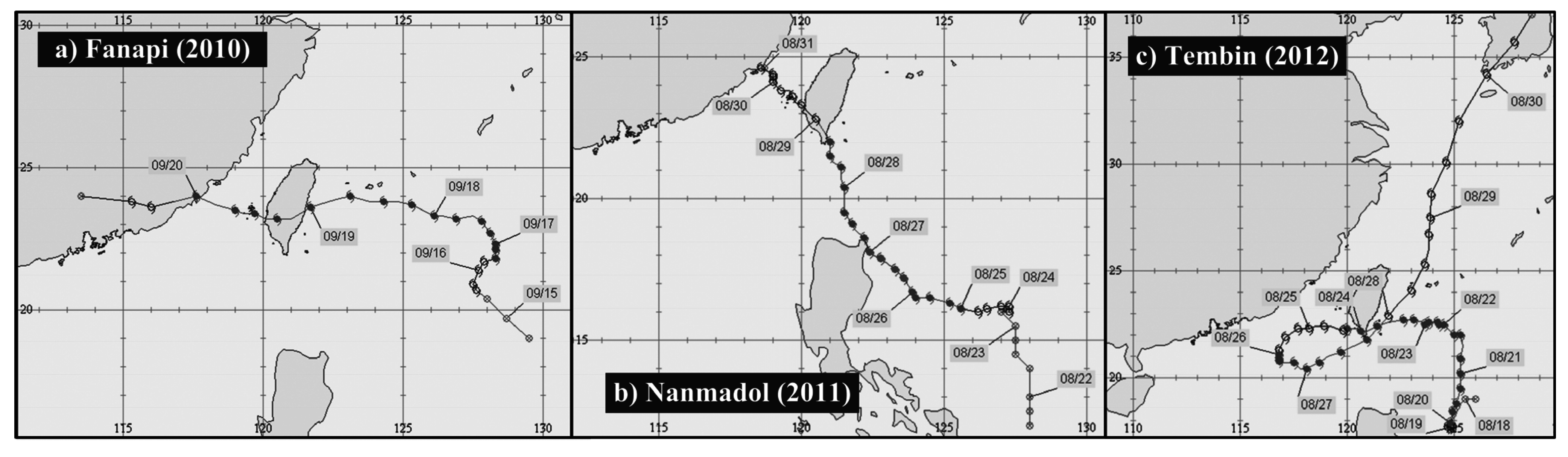
3.1. Study Area and Data

Figure 3 depicts the experimental site at the Dawu gauge station (22°21′27″ N, 120°53′44″ E; elevation 8.1 m) in Taiwan, located along the main path of the Northwestern Pacific tropical typhoons. This study considered 28 typhoon events that affected Dawu station between 2001 and 2012 (Table 1). The climatology of typhoons and the ground weather data of the Dawu station were collected from the Central Weather Bureau of Taiwan. Typhoon characteristics, namely the pressure, latitude, and longitude of the typhoon center; radius of the typhoon; and maximal wind speed near the typhoon center, were collected for analysis. The ground weather data comprised the air pressure, temperature, dew point temperature, relative humidity, and vapor pressure of the ground; surface wind speed and direction; and surface rain rate.

Figure 3. Dawu gauge station and the track of Typhoon Morakot (2009).

Figure 3. Dawu gauge station and the track of Typhoon Morakot (2009).

Table 1. The 28 typhoon events considered in this study.

Year	Typhoon Name	Year	Typhoon Name
2001	Lekima	2007	Pabuk, Wutip, Sepat, Wipha, Krosa
2002	Nakri	2008	Kalmaegi, Fung-Wong, Sinlaku
2003	Morakot, Dujuan, Melor	2009	Morakot
2004	Mindulle, Aere, Nanmadol	2010	Fanapi
2005	Haitang, Matsa, Talim, Longwang	2011	Nanmadol
2006	Chanchu, Billis, Kaemi, Bopha	2012	Tembin

Table 1. The 28 typhoon events considered in this study.

Year	Typhoon Name	Year	Typhoon Name
2001	Lekima	2007	Pabuk, Wutip, Sepat, Wipha, Krosa
2002	Nakri	2008	Kalmaegi, Fung-Wong, Sinlaku
2003	Morakot, Dujuan, Melor	2009	Morakot
2004	Mindulle, Aere, Nanmadol	2010	Fanapi
2005	Haitang, Matsa, Talim, Longwang	2011	Nanmadol
2006	Chanchu, Billis, Kaemi, Bopha	2012	Tembin

3.2. Data Division

The typhoon characteristics data comprised 1462 records measured at hourly intervals. Table 2 lists the mean, minimal, and maximal values of the data attributes. To build the ANN–PAC model, the data sets were classified into training and testing sets. The typhoon events that occurred between 2001 and 2008 were used for training. In addition, Typhoons Morakot (2009) and Fanapi (2010) were used as a validation set, and Typhoons Nanmadol (2011) and Tembin (2012) were used as a testing set. Figure 3 and Figure 4 display the historical tracks of these typhoons.

Table 2. Range and average values of data attributes.

Data Attribute	Range	Mean
Pressure at typhoon center (hPa)	912.0−1000.0	964.3
Latitude (°N) of typhoon center (degree)	12.0−27.8	23.2
Longitude (°E) of typhoon center (degree)	115.3−128.1	121.5
Radius of typhoon (km)	0−300.0	207.7
Maximum wind speed near typhoon center (m℘s−1)	7.0−16.0	11.9
Air pressure on the ground (hPa)	967.2−1011.3	995.0
Temperature on the ground (°C)	23.1−35.8	27.0
Dew point temperature on the ground (°C)	18.1−28.0	24.1
Relative humidity on the ground (%)	40.0−100.0	85.5
Vapor pressure on the ground (hPa)	20.8−37.8	30.2
Surface wind speed (m·s−1)	0.0−20.2	3.6
Surface wind direction	0.0−360.0	165.7
Surface rain rate (mm·h−1)	0.0−103.0	4.5

Table 2. Range and average values of data attributes.

Data Attribute	Range	Mean
Pressure at typhoon center (hPa)	912.0−1000.0	964.3
Latitude (°N) of typhoon center (degree)	12.0−27.8	23.2
Longitude (°E) of typhoon center (degree)	115.3−128.1	121.5
Radius of typhoon (km)	0−300.0	207.7
Maximum wind speed near typhoon center (m℘s−1)	7.0−16.0	11.9
Air pressure on the ground (hPa)	967.2−1011.3	995.0
Temperature on the ground (°C)	23.1−35.8	27.0
Dew point temperature on the ground (°C)	18.1−28.0	24.1
Relative humidity on the ground (%)	40.0−100.0	85.5
Vapor pressure on the ground (hPa)	20.8−37.8	30.2
Surface wind speed (m·s−1)	0.0−20.2	3.6
Surface wind direction	0.0−360.0	165.7
Surface rain rate (mm·h−1)	0.0−103.0	4.5

Figure 4. Typhoon tracks of (a) Fanapi (2010); (b) Nanmadol (2011); and (c) Tembin (2012).

Figure 4. Typhoon tracks of (a) Fanapi (2010); (b) Nanmadol (2011); and (c) Tembin (2012).

3.3. Modeling Using ANN–PAC

This study employed a widely used MLP neural network for forecasting precipitation at the study site. Figure 1 depicts the input–output patterns of the MLP model. The model inputs contained 13 meteorological attributes, and the target output is the amount of rain in the next 1 h. As stated, the MLP ANN comprises the learning rate, momentum, and number of neurons in the hidden layer. To construct the MLP, sigmoid and linear activity functions were used in the hidden and output layers, respectively. The proposed ANN–PAC approach was applied for investigating the optimal parameter combination.

The ranges of the three aforementioned parameters in the MLP network were set. Because the momentum and learning rate are theoretically in the range of [0,1], 0.1 and 1.0 were set as their lower and upper limits. For the number of hidden neurons, we defined the ratio of hidden neurons as the ratio of the number of neurons in the hidden layer to the number of records in a training set. This ratio ranged between 0.01 and 0.1.

In addition, the number of increments between the maximal and minimal values, assumed as 10 equal-sized intervals, is the same for all three calibrated parameters. The effect of the number of increments on the prediction accuracy is evaluated in Section 4.4.

During training, the MLP network was trained using a training set. The model prediction errors, computed using the relative root mean squared error (RRMSE), were then calculated for each iterative process using a validation set:

$$\text{RRMSE}=\sqrt{\frac{1}{N}{\displaystyle \sum _{i=1}^N{\left(O_i^{\text{pre}}-O_i^{\text{obs}}\right)}^2}}/{\overline{O}}^{\text{obs}}$$

(2)

where $O_i^{\text{pre}}$ and $O_i^{\text{obs}}$ are the predicted and observed values at record i, respectively; ${\overline{O}}^{\text{obs}}$ is the average of the observations and N is the number of records.

The optimal parameter values were obtained after calibrating the parameters using the ANN–PAC approach: the ratio of hidden neurons = 0.02, momentum = 0.2, and learning rate = 0.6. Figure 5 displays the RRMSE results of the ANN–PAC model using a validation set. To three-dimensionally depict the RRMSE variations, one of three parameters was fixed; for example, in Figure 5a, the RRMSE variations were plotted at various learning rate and momentum values and a fixed hidden neurons ratio of 0.02.

Figure 5. Three-dimensional plots of relative root mean squared error (RRMSE) variations at (a) a fixed hidden neurons ratio of 0.02, (b) a fixed momentum of 0.2; and (c) a fixed learning rate of 0.6.

Figure 5. Three-dimensional plots of relative root mean squared error (RRMSE) variations at (a) a fixed hidden neurons ratio of 0.02, (b) a fixed momentum of 0.2; and (c) a fixed learning rate of 0.6.

4. Evaluations and Comparisons

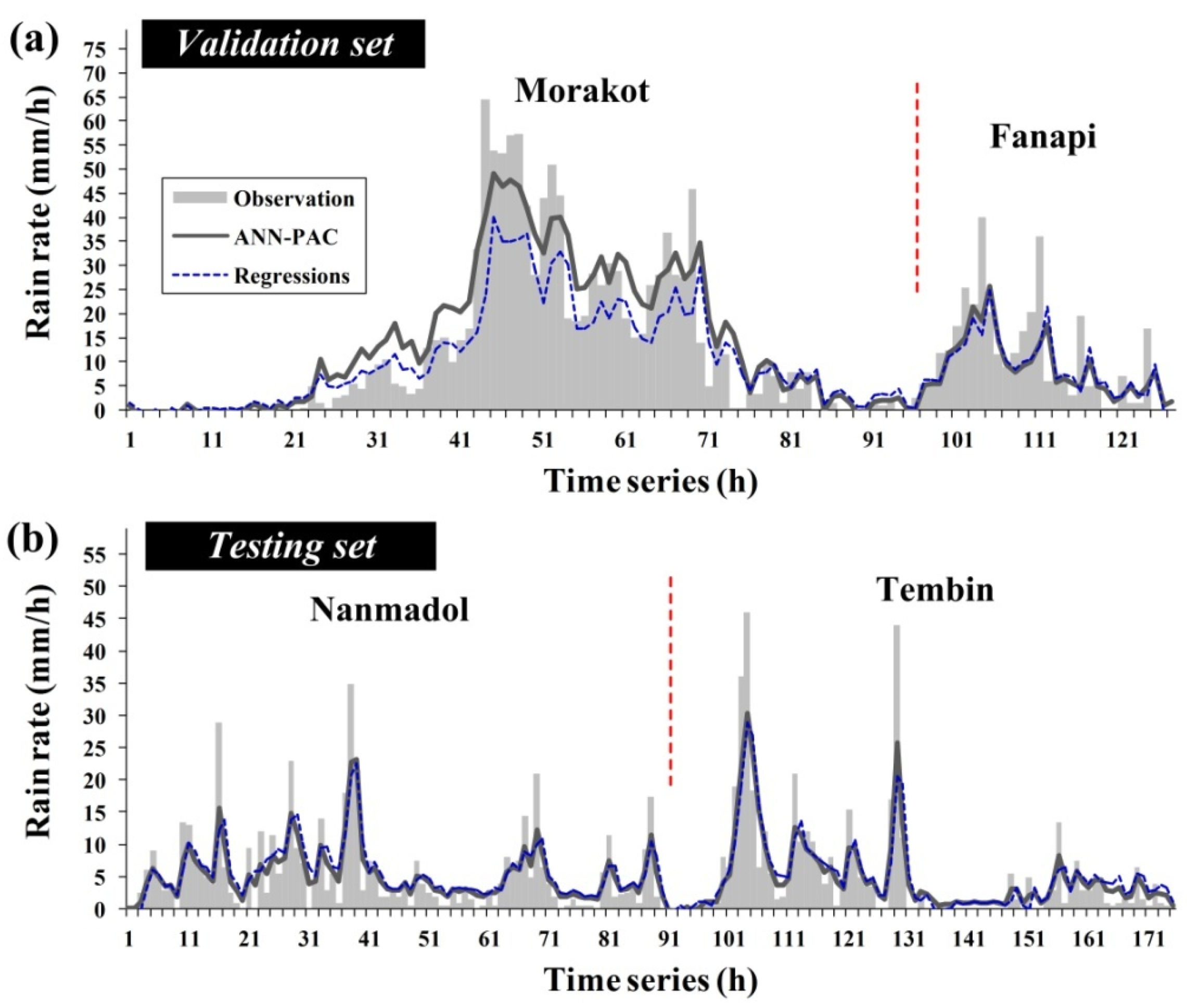
4.1. Results

The traditional multiple linear regression model was selected as the benchmark for comparing the accuracy of the ANN–PAC model. Unlike ANNs, which typically require a trial-and-error or heuristic parameter calibration approach, the coefficients in regression analysis can be efficiently calculated using the matrix algebra regardless of the number of data points and variables. Figure 6a presents the 1-h-ahead rain variations of the observations and predictions obtained using a validation set (i.e., Typhoons Morakot and Fanapi) for the ANN–PAC and regression-based models, and Figure 6b presents the 1-h-ahead rain variations of the observations and predictions obtained using a testing set (i.e., Typhoons Nanmadol and Tembin). The predictions obtained using the ANN–PAC model were highly consistent with the observed data, compared with the regression-based models for both the validation and testing sets. To evaluate the constructed ANN–PAC models, we designed two model scenarios, as described in the next section.

Figure 6. Simulation results of 1-h-ahead predictions for hyetograph using: (a) the validation set and (b) the testing set.

Figure 6. Simulation results of 1-h-ahead predictions for hyetograph using: (a) the validation set and (b) the testing set.

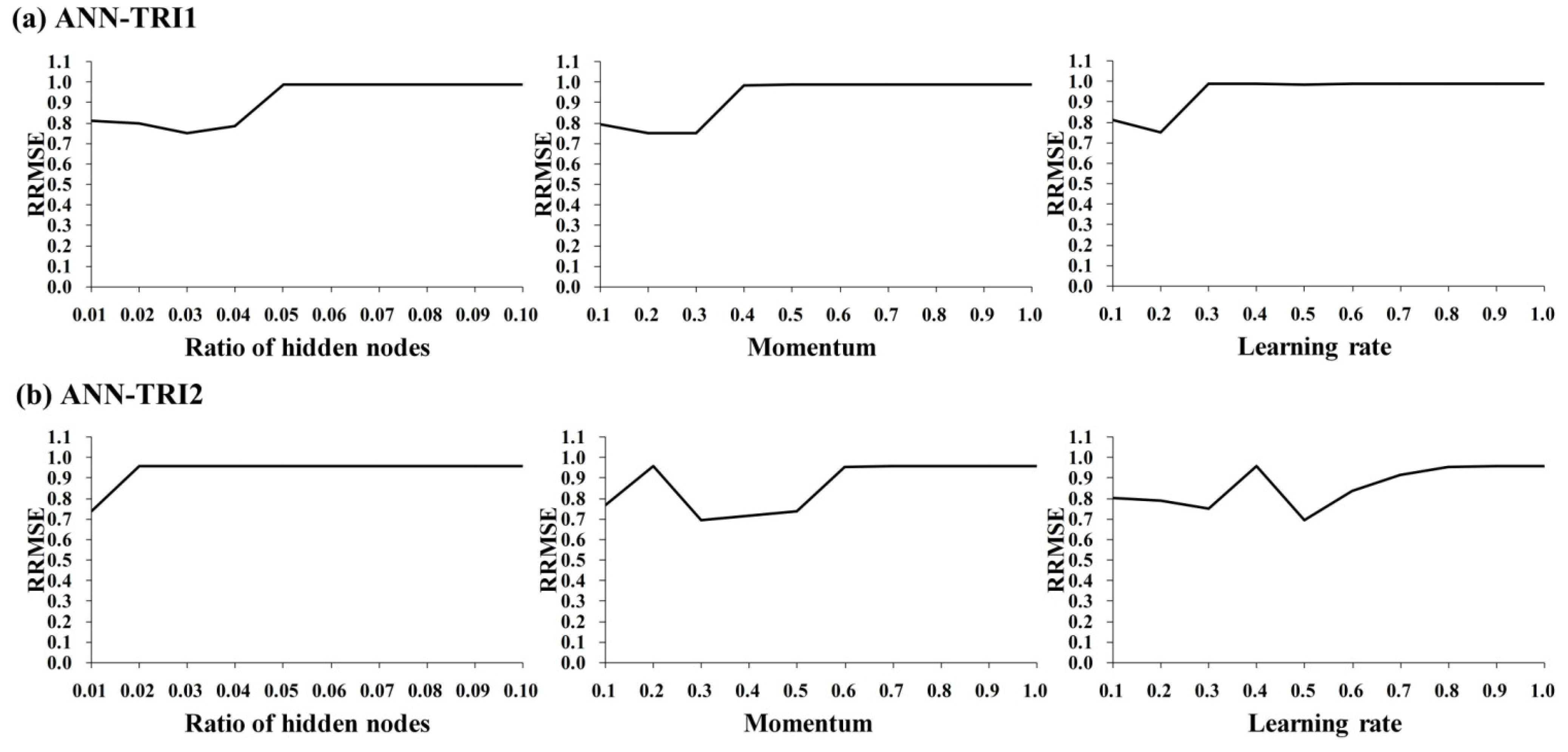
4.2. Model Scenarios

ANN model parameters are typically fixed on the basis of experience. As shown in Figure 2, the parameters of the proposed methodology can be manually tuned using trial-and-error calibration. Herein, the process of calibrating ANN-based MLP parameters by using a validation set is described. As illustrated in Figure 7, the initial momentum and learning rate values were set first. After sensitivity analysis, the “local” optimal ratio of the hidden neurons was calibrated. Subsequently, the local optimal ratio of the hidden neurons and the initial learning rate, which had been calibrated, were fixed, and the local optimal momentum value was calculated through sensitivity analysis. Subsequently, the local optimal ratio of hidden neurons and momentum value were fixed, and the suitable learning rate was calculated through sensitivity analysis.

In this study, two scenarios with differing initial parameters were designed using the aforementioned trial-and-error method. The first scenario, ANN–TRI1, used initial values of 0.02, 0.2, and 0.2 for the ratio of hidden neurons, momentum, and learning rate, respectively. The second scenario, ANN–TRI2, used initial values of 0.05, 0.5 and 0.5, respectively. The ranges of these parameters are the same as those in Section 3.3. Figure 8 plots the sensitivity results of the MLP parameters for the ANN–TRI1 and ANN–TRI2 models. The calibrated values of the three parameters are (0.01, 0.3, 0.5) and (0.03, 0.2, 0.2) for ANN–TRI1 and ANN–TRI2, respectively.

Figure 7. Trial-and-error calibration of ANN parameters.

Figure 7. Trial-and-error calibration of ANN parameters.

Figure 8. Sensitivity results of MLP parameters by using a validation set for two MLP ANN models based on a trial-and-error calibration method: (a) ANN–TRI1; and (b) ANN–TRI2.

Figure 8. Sensitivity results of MLP parameters by using a validation set for two MLP ANN models based on a trial-and-error calibration method: (a) ANN–TRI1; and (b) ANN–TRI2.

4.3. Performance Levels and Comparisons

To assess the performance levels from the obtained results, the relative mean absolute error (RMAE), RRMSE, and coefficient of correlation (r) were calculated:

$$\text{RMAE}=\left(\frac{1}{N}{\displaystyle \sum _{i=1}^N\left|O_i^{\text{pre}}-O_i^{\text{obs}}\right|}\right)/{\overline{O}}^{\text{obs}}$$

(3)

$$\text{r}=\frac{{\displaystyle \sum _{i=1}^N\left(O_i^{\text{obs}}-{\overline{O}}^{\text{obs}}\right)\left(O_i^{\text{pre}}-{\overline{O}}^{\text{pre}}\right)}}{\sqrt{{\displaystyle \sum _{i=1}^N{\left(O_i^{\text{obs}}-{\overline{O}}^{\text{obs}}\right)}^2}{\displaystyle \sum _{i=1}^N{\left(O_i^{\text{pre}}-{\overline{O}}^{\text{pre}}\right)}^2}}}$$

(4)

where ${\overline{O}}^{\text{pre}}$ is the average of the predictions. Low RMAE and RRMSE values and high r values typically indicate favorable performance levels. Precise predictions are those whose RMAE, and RRMSE are nearly 0 and r values are nearly 1.

The predictions of the ANN–PAC, ANN–TRI1, ANN–TRI2, and regression models were compared using these performance criteria. Table 3 lists the results for the four models obtained using RMAE, RRMSE, and r performance criteria calculated by the validation and testing sets. The RMAE was computed using a term-by-term comparison of the error in the prediction and the actual value of the variable. Thus, the RMAE is an unbiased statistic for measuring the predictive capability of a model [43]. For the validation and testing sets, the RMAE and RRMSE results for the ANN–PAC model were lower than those for the ANN–TRI1, ANN–TRI2, and regression models, implying that ANN–PAC exhibited relatively few prediction errors and lower bias measures with respect to the actual values, possibly because trial-and-error calibrations cannot be performed for all variables simultaneously but rather separately, which is a time-intensive process. Moreover, because the interaction between parameters cannot be determined, this method cannot obtain global optimal solutions [20]. The r performance levels suggested that the ANN–PAC and regression models successfully exploited the relationship between the observed and predicted rainfalls. In addition, by comparing the ANN–PAC results obtained for the validation and testing sets, we observed that the performance levels obtained using the validation set were slightly higher than those obtained using the testing set. Therefore, we concluded that the generalizability of the constructed ANN–PAC model can be calibrated using the training–validation–testing procedure for applications in precipitation forecasting.

Table 3. Performance levels of the various models assessed by using the validation set Testing sets.

Subset	Model	Performance
		RMAE	RRMSE	r
Validation set	ANN-PAC	0.397	0.575	0.886
	ANN-TRI1	0.528	0.750	0.817
	ANN-TRI2	0.482	0.695	0.832
	Regressions	0.441	0.708	0.859
Testing set	ANN-PAC	0.429	0.685	0.824
	ANN-TRI1	0.557	0.901	0.742
	ANN-TRI2	0.555	0.895	0.733
	Regressions	0.581	0.880	0.755

Table 3. Performance levels of the various models assessed by using the validation set Testing sets.

Subset	Model	Performance
		RMAE	RRMSE	r
Validation set	ANN-PAC	0.397	0.575	0.886
	ANN-TRI1	0.528	0.750	0.817
	ANN-TRI2	0.482	0.695	0.832
	Regressions	0.441	0.708	0.859
Testing set	ANN-PAC	0.429	0.685	0.824
	ANN-TRI1	0.557	0.901	0.742
	ANN-TRI2	0.555	0.895	0.733
	Regressions	0.581	0.880	0.755

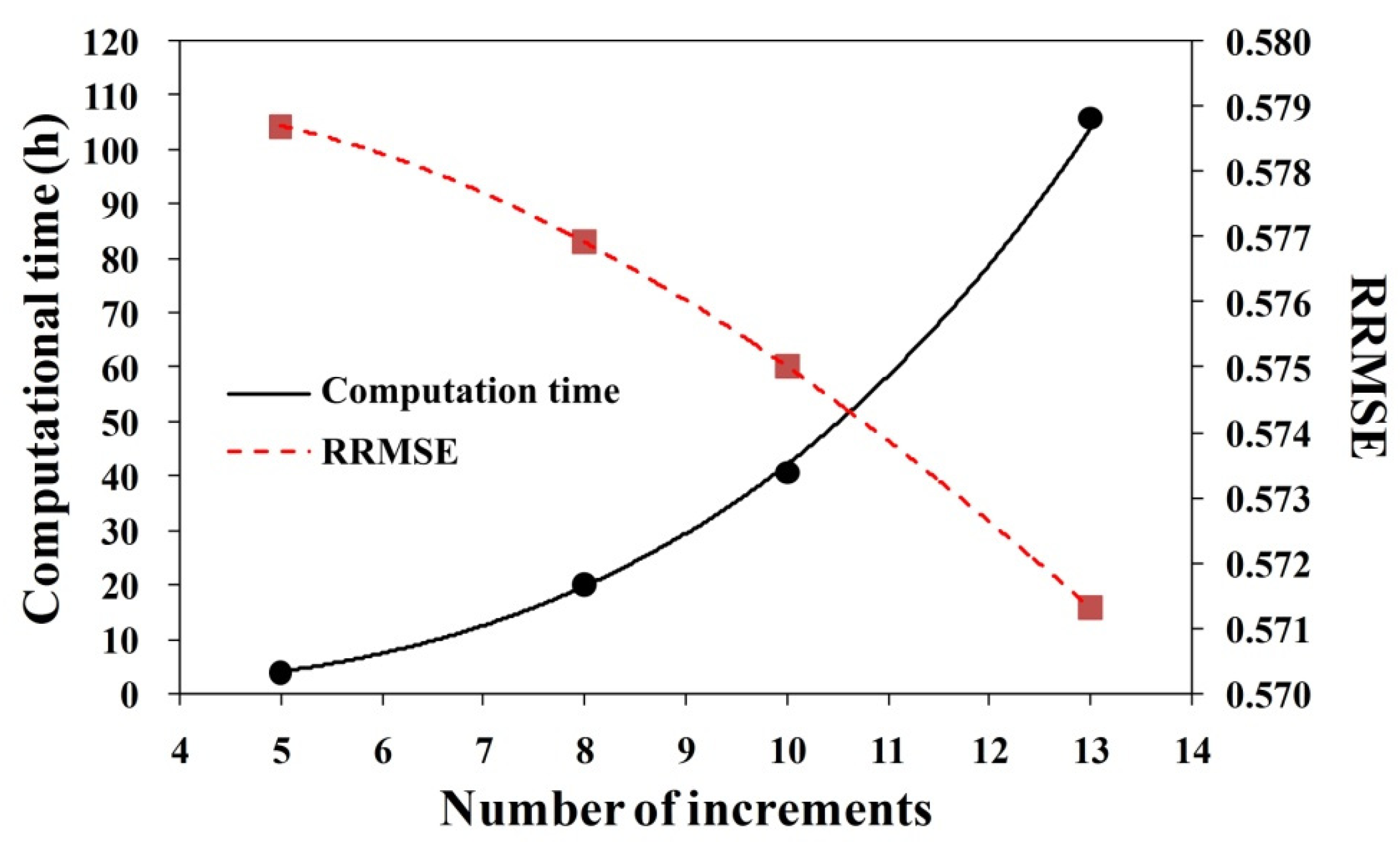
4.4. Effects of the Number of Increments

As stated in Section 3.3, the number of increments between the minimal and maximal values for each parameter was 10. To investigate the effect of the number of increments on the prediction ability and computation efficiency, the number of increments were varied as 5, 8, 10, and 13. Figure 9 illustrates the relationships among RRMSE prediction errors by using a validation set, computational time, and the number of increments. As the number of increments increases, the computing efficiency decreases because of a considerable increase in computational time, whereas the prediction errors decrease because of the increased capability of finding the optimal solution.

Figure 9. Effect of increment numbers on computational time and prediction errors.

Figure 9. Effect of increment numbers on computational time and prediction errors.

5. Conclusions

ANNs are widely applied in engineering solutions. When constructing ANN-based models, a considerable number of model parameters must be calibrated, and the trial-and-error method is frequently employed for calibration during ANN training. This paper presents ANN models for 1-h-ahead rainfall forecasting, in which the training model parameters are adjusted using the proposed PAC approach. The classical MLP ANN model was used to verify the utility of the proposed approach. The MLP-based ANN comprises three parameters: the learning rate, momentum, and number of nodes in the hidden layer.

Observed typhoon characteristics and ground weather data at the Dawu gauge station in Taitung, Taiwan, were the study data. To compare the accuracy of ANN–PAC, traditional multiple linear regression was selected as the benchmark. In addition, two ANN models based on a trial-and-error calibration method, ANN–TRI1 and ANN–TRI2, were realized by manually tuning the parameters. The results clarify that the ANN–PAC model yielded more reliable results than ANN–TRI1, ANN–TRI2, and the regression models. Moreover, as the number of increments within the parameter ranges increased, the computing efficiency of the ANN–PAC model decreased because of considerable increase in the computational time, whereas the prediction errors of the model decreased because of the model’s increased capability of finding the optimal solution. Therefore, a high number of increments within parameter ranges must be used in applications where accuracy is critical, whereas a low number must be used in applications where computing efficiency is essential.

References

1. Lee, C.S.; Huang, L.R.; Shen, H.S.; Wang, S.T. A climatology model for forecasting typhoon rainfall in Taiwan. Nat. Hazards 2006, 37, 87–105. [Google Scholar] [CrossRef]
2. McCulloch, W.S.; Pitts, W. A logical calculus of the ideas imminent in nervous activity. Bull. Math. Biophys. 1943, 5, 115–133. [Google Scholar] [CrossRef]
3. Rumelhart, D.E.; Hinton, G.E.; Williams, R.J. Learning Internal Representations by Error Propagation. In Parallel Distributed Processing; Rumelhart, D.E., McClelland, J.L., Eds.; MIT Press: Cambridge, UK, 1986. [Google Scholar]
4. Asklany, S.A.; Elhelow, K.; Youssef, I.K.; El-wahab, M.A. Rainfall events prediction using rule-based fuzzy inference system. Atmos. Res. 2011, 101, 228–236. [Google Scholar] [CrossRef]
5. Babovic, V. Data mining in hydrology. Hydrol. Process. 2005, 19, 1511–1515. [Google Scholar] [CrossRef]
6. Chang, F.J.; Chiang, Y.M.; Tsai, M.J.; Shieh, M.C.; Hsu, K.L.; Sorooshian, S. Watershed rainfall forecasting using neuro-fuzzy networks with the assimilation of multi-sensor information. J. Hydrol. 2014, 508, 374–384. [Google Scholar] [CrossRef]
7. Cheng, C.; Wang, S.; Chau, K.W.; Wu, X. Parallel discrete differential dynamic programming for multireservoir operation. Environ. Model. Softw. 2014, 57, 152–164. [Google Scholar] [CrossRef]
8. Chau, K.W.; Wu, C.L.; Li, Y.S. Comparison of several flood forecasting models in Yangtze River. J. Hydrol. Eng. 2005, 10, 485–491. [Google Scholar] [CrossRef]
9. Kecman, V. Learning and Soft Computing: Support Vector Machines, Neural Networks, and Fuzzy Logic Models; MIT Press: Cambridge, UK, 2001. [Google Scholar]
10. Liu, W.C.; Chung, C.E. Enhancing the predicting accuracy of the water stage using a physical-based model and an artificial neural network-genetic algorithm in a river system. Water 2014, 6, 1642–1661. [Google Scholar] [CrossRef]
11. Minns, W.; Hall, M.J. Artificial neural networks as rainfall-runoff models. Hydrol. Sci. J. 1996, 41, 399–417. [Google Scholar] [CrossRef]
12. Surridge, B.W.J.; Bizzi, S.; Castelletti, A. A framework for coupling explanation and prediction in hydroecological modelling. Environ. Model. Softw. 2014, 61, 274–286. [Google Scholar] [CrossRef]
13. Taormina, R.; Chau, K.W.; Sethi, R. Artificial neural network simulation of hourly groundwater levels in a coastal aquifer system of the Venice lagoon. Eng. Appl. Artif. Intell. 2012, 25, 1670–1676. [Google Scholar] [CrossRef]
14. Vojinovic, Z.; Kecman, V.; Babovic, V. Hybrid approach for modeling wet weather response in wastewater systems. J. Water Resour. Plan. Manag. 2003, 129, 511–521. [Google Scholar] [CrossRef]
15. Wang, W.C.; Xu, D.M.; Chau, K.W.; Chen, S. Improved annual rainfall-runoff forecasting using PSO–SVM model based on EEMD. J. Hydroinform. 2013, 15, 1377–1390. [Google Scholar]
16. Wei, C.C. RBF neural networks combined with principal component analysis applied to quantitative precipitation forecast for a reservoir watershed during typhoon periods. J. Hydrometeorol. 2012, 13, 722–734. [Google Scholar] [CrossRef]
17. Wei, C.C. Soft computing techniques in ensemble precipitation nowcast. Appl. Soft Comput. 2013, 13, 793–805. [Google Scholar] [CrossRef]
18. Wei, C.C.; Hsu, N.S.; Huang, C.L. Two-Stage pumping control model for flood mitigation in inundated urban drainage basins. Water Resour. Manag. 2014, 28, 425–444. [Google Scholar] [CrossRef]
19. Wu, C.L.; Chau, K.W. Prediction of rainfall time series using modular soft computing methods. Eng. Appl. Artif. Intell. 2013, 26, 997–1007. [Google Scholar] [CrossRef]
20. Cai, H.; Lye, L.M.; Khan, A. Flood Forecasting on the Humber River using an Artificial Neural Network Approach. In Proceedings of the 2009 Canadian Society for Civil Engineering Annual Conference; Canadian Society for Civil Engineering: Montreal, Canada, 2009; Volume 2, pp. 611–620. [Google Scholar]
21. Dai, H.C.; Macbeth, C. Effects of learning parameters on learning procedure and performance of a BPNN. Neural Netw. 1997, 10, 1505–1521. [Google Scholar] [CrossRef]
22. Maier, H.R.; Dandy, G.C. Neural networks for the prediction and forecasting of water resources variables: A review of modelling issues and applications. Environ. Modell. Softw. 2000, 15, 101–124. [Google Scholar] [CrossRef]
23. Chen, W.; Chau, K.W. Intelligent manipulation and calibration of parameters for hydrological models. Int. J. Environ. Pollut. 2006, 28, 432–447. [Google Scholar] [CrossRef]
24. Dawson, C.W.; Abrahart, R.J.; Shamseldin, A.Y.; Wilby, R.L. Flood estimation at ungauged sites using artificial neural networks. J. Hydrol. 2006, 319, 391–409. [Google Scholar] [CrossRef]
25. Jacobs, R.A. Increased rates of convergence through learning rate adaptation. Neural Netw. 1988, 1, 295–307. [Google Scholar] [CrossRef]
26. Kamruzzaman, M.; Shahriar, M.S.; Beecham, S. Assessment of short term rainfall and stream flows in South Australia. Water 2014, 6, 3528–3544. [Google Scholar] [CrossRef]
27. Lin, G.F.; Jhong, B.C. A real-time forecasting model for the spatial distribution of typhoon rainfall. J. Hydrol. 2015, 521, 302–313. [Google Scholar] [CrossRef]
28. Pasini, A.; Pelino, V.; Potestà, S. A neural network model for visibility nowcasting from surface observations: Results and sensitivity to physical input variables. J. Geophys. Res. 2001, 106, 14951–14959. [Google Scholar] [CrossRef]
29. Pasini, A.; Langone, R. Attribution of precipitation changes on a regional scale by neural network modeling: A case study. Water 2010, 2, 321–332. [Google Scholar] [CrossRef]
30. Pasini, A.; Langone, R. Influence of circulation patterns on temperature behavior at the regional scale: A case study investigated via neural network modeling. J. Clim. 2012, 25, 2123–2128. [Google Scholar] [CrossRef]
31. Pasini, A.; Modugno, G. Climatic attribution at the regional scale: A case study on the role of circulation patterns and external forcings. Atmos. Sci. Lett. 2013, 14, 301–305. [Google Scholar] [CrossRef]
32. Wei, C.C. Forecasting surface wind speeds over offshore islands near Taiwan during tropical cyclones: Comparisons of data-driven algorithms and parametric wind representations. J. Geophys. Res. Atmos. 2015, 120, 1826–1847. [Google Scholar] [CrossRef]
33. Zhang, Y.; Li, G. Long-term evolution of cones of depression in shallow aquifers in the North China Plain. Water 2013, 5, 677–697. [Google Scholar] [CrossRef]
34. Sheela, K.G.; Deepa, S.N. Review on methods to fix number of hidden neurons in neural networks. Math. Probl. Eng. 2013, 2013. [Google Scholar] [CrossRef]
35. Maier, H.R.; Dandy, G.C. The effect of internal parameters and geometry on the performance of back-propagation neural networks: An empirical study. Environ. Model. Softw. 1998, 13, 193–209. [Google Scholar] [CrossRef]
36. Maier, H.R.; Jain, A.; Dandy, G.C.; Sudheer, K. Methods used for the development of neural networks for the prediction of water resource variables in river systems: current status and future directions. Environ. Model. Softw. 2010, 25, 891–909. [Google Scholar] [CrossRef]
37. Panchal, G.; Ganatra, A.; Kosta, Y.P.; Panchal, D. Behaviour analysis of multilayer perceptrons with multiple hidden neurons and hidden layers. Int. J. Comput. Theor. Eng. 2011, 3, 332–337. [Google Scholar] [CrossRef]
38. Patra, J.C.; van den Bos, A. Auto-calibration and -compensation of a capacitive pressure sensor using multilayer perceptrons. ISA Trans. 2000, 39, 175–190. [Google Scholar] [CrossRef]
39. Kurt, I.; Ture, M.; Kurum, A.T. Comparing performances of logistic regression, classification and regression tree, and neural networks for predicting coronary artery disease. Expert Syst. Appl. 2008, 34, 366–374. [Google Scholar] [CrossRef]
40. Imrie, C.E.; Durucan, S.; Korre, A. River flow prediction using artificial neural networks: Generalization beyond the calibration range. J. Hydrol. 2000, 233, 138–153. [Google Scholar] [CrossRef]
41. Pasini, A. Artificial neural networks for small dataset analysis. J. Thorac. Dis. 2015, 7, 953–960. [Google Scholar] [PubMed]
42. Prechelt, L.; Orr, G.B. Early Stopping−But When? In Neural Networks: Tricks of the Trade. Lecture Notes in Computer Science; Montavon, G., Müller, K.R., Eds.; Springer: Berlin, Germany; Heidelberg, Germany, 2012; pp. 53–67. [Google Scholar]
43. Hu, T.S.; Lam, K.C.; Ng, S.T. River flow time series prediction with a range dependent neural network. Hydrol. Sci. J. 2001, 46, 729–745. [Google Scholar] [CrossRef]