Spatial Disaggregation of Areal Rainfall Using Two Different Artificial Neural Networks Models

Abstract

The objective of this study is to develop artificial neural network (ANN) models, including multilayer perceptron (MLP) and Kohonen self-organizing feature map (KSOFM), for spatial disaggregation of areal rainfall in the Wi-stream catchment, an International Hydrological Program (IHP) representative catchment, in South Korea. A three-layer MLP model, using three training algorithms, was used to estimate areal rainfall. The Levenberg–Marquardt training algorithm was found to be more sensitive to the number of hidden nodes than were the conjugate gradient and quickprop training algorithms using the MLP model. Results showed that the networks structures of 11-5-1 (conjugate gradient and quickprop) and 11-3-1 (Levenberg-Marquardt) were the best for estimating areal rainfall using the MLP model. The networks structures of 1-5-11 (conjugate gradient and quickprop) and 1-3-11 (Levenberg–Marquardt), which are the inverse networks for estimating areal rainfall using the best MLP model, were identified for spatial disaggregation of areal rainfall using the MLP model. The KSOFM model was compared with the MLP model for spatial disaggregation of areal rainfall. The MLP and KSOFM models could disaggregate areal rainfall into individual point rainfall with spatial concepts.

1. Introduction

Rainfall is a necessary input for the design of hydrologic and hydraulic systems. Rainfall can be either measured or generated using stochastic simulation [1]. The variability of rainfall has been acknowledged as a reason for the uncertainties in hydrologic applications. To minimize uncertainties calls for methods that improve the reliability of rainfall estimation by combining rainfall information from different sources [2].

Areal rainfall is the average rainfall over the region under consideration and is estimated by one of the popular methods, such as arithmetic mean, Thiessen polygon, isohyetal, spline, kriging, and copula amongst others [3,4,5]. The arithmetic mean method is the simplest one for determining areal rainfall. The Thiessen polygon method assumes a linear variation in rainfall between two neighboring stations and polygons are constructed which are essentially areal weights. This method is considered more accurate than the arithmetic mean method. The isohyetal method involves construction of isohyets using observed depths at rainfall stations and assumes a linear variation between two adjacent isohyets [4,6] The spline method is an interpolation method that divides interpolation intervals into small subintervals and each of these subintervals is interpolated by using the third-degree polynomial [7,8]. The kriging method is an optimal interpolator, based on regression against observed rainfall values of surrounding rainfall points, weighted according to spatial covariance values [5,9]. The copula method can be employed to describe the dependencies on an n dimensional unit cube (uniform) among n random variables. Description of the spatial dependence structure independent of the marginal distribution is one of the most attractive features of copulas [10,11].

Rainfall disaggregation can be both temporal and spatial. Temporal rainfall disaggregation entails disaggregating hourly, daily, or longer duration rainfall into short time rainfall, and many techniques have been proposed [12,13,14,15,16,17,18,19,20,21,22,23,24,25]. Techniques for spatial rainfall disaggregation using various interpolations and global climate models (GCMs) scenarios have been proposed. However, relatively limited research has been reported on spatial rainfall disaggregation as compared with temporal rainfall disaggregation [26,27,28,29].

Artificial neural networks (ANNs) are a robust computational method that has been primarily used for pattern recognition, classification, and prediction [30]. The main advantage of the ANNs as an alternative of the physical and conventional methods is that we do not need an explicit description in mathematical terms for the complex processes of the system under consideration [31,32,33]. Therefore, ANNs can generalize the strong nonlinear patterns of natural phenomena, including aggregation and disaggregation of rainfall with stabilization.

During the past decades, a variety of ANNs have been developed and applied for temporal rainfall disaggregation [1,34,35]. In this study, two ANN models, including multilayer perceptron (MLP) and Kohonen self-organizing feature map (KSOFM), have been applied to estimate spatial disaggregation of areal rainfall in the Wi-stream catchment. MLP and KSOFM have been used effectively to model and forecast hydrologic time series. Recently, outstanding results using the MLP and KSOFM models in the fields of modeling and forecasting, including evapotranspiration, pan evaporation, river flood, precipitation downscaling, dew point temperature, soil temperature, and water level and so on, have been obtained [31,36,37,38,39,40,41,42,43,44,45,46,47]. In this study, areal rainfall is the average rainfall over the region under consideration and is estimated using the kriging method. Spatial disaggregation of areal rainfall, therefore, refers to the process of estimating point rainfall corresponding to individual rainfall stations. Although there have been many investigations using ANNs, their application for spatial disaggregation of areal rainfall has been limited. The mathematical formulas based on the spatial disaggregation of areal rainfall on the catchment cannot be derived or developed using conventional methods, including simple regression analysis. Therefore, the strong nonlinear behavior in nature, such as spatial disaggregation of areal rainfall, can be overcome using the ANNs successfully in this study.

The objective of this study therefore is to develop and apply two ANN models, including multilayer perceptron (MLP) and Kohonen self-organizing feature map (KSOFM), for spatial disaggregation of areal rainfall in the Wi-stream catchment, an IHP representative catchment, in South Korea. The paper is organized as follows: The second part describes ANNs, including MLP and KSOFM. The third part describes a case study, including data used and study area. The forth part presents application and results. Conclusions are presented in the last part of the paper.

2. Artificial Neural Networks

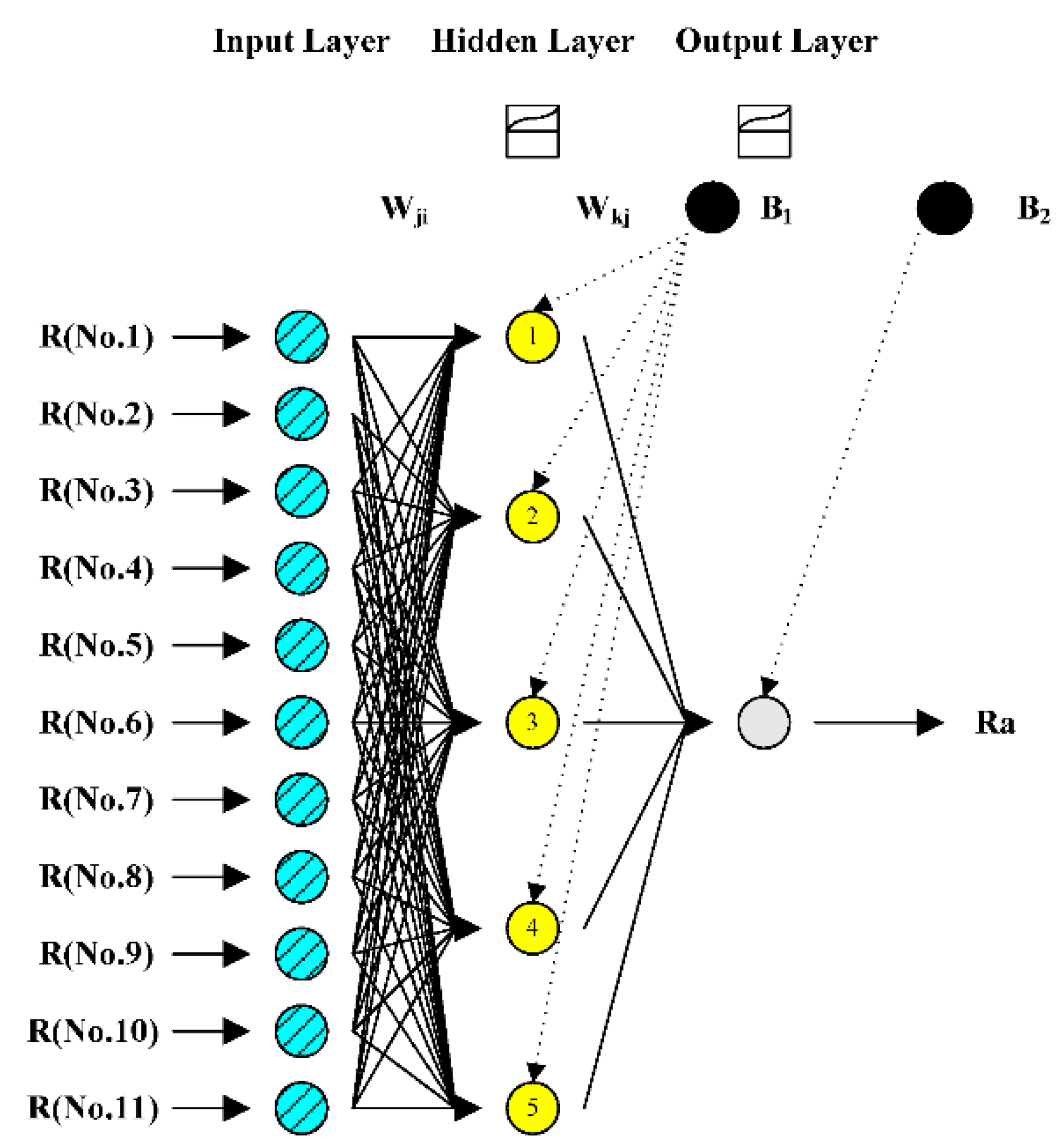
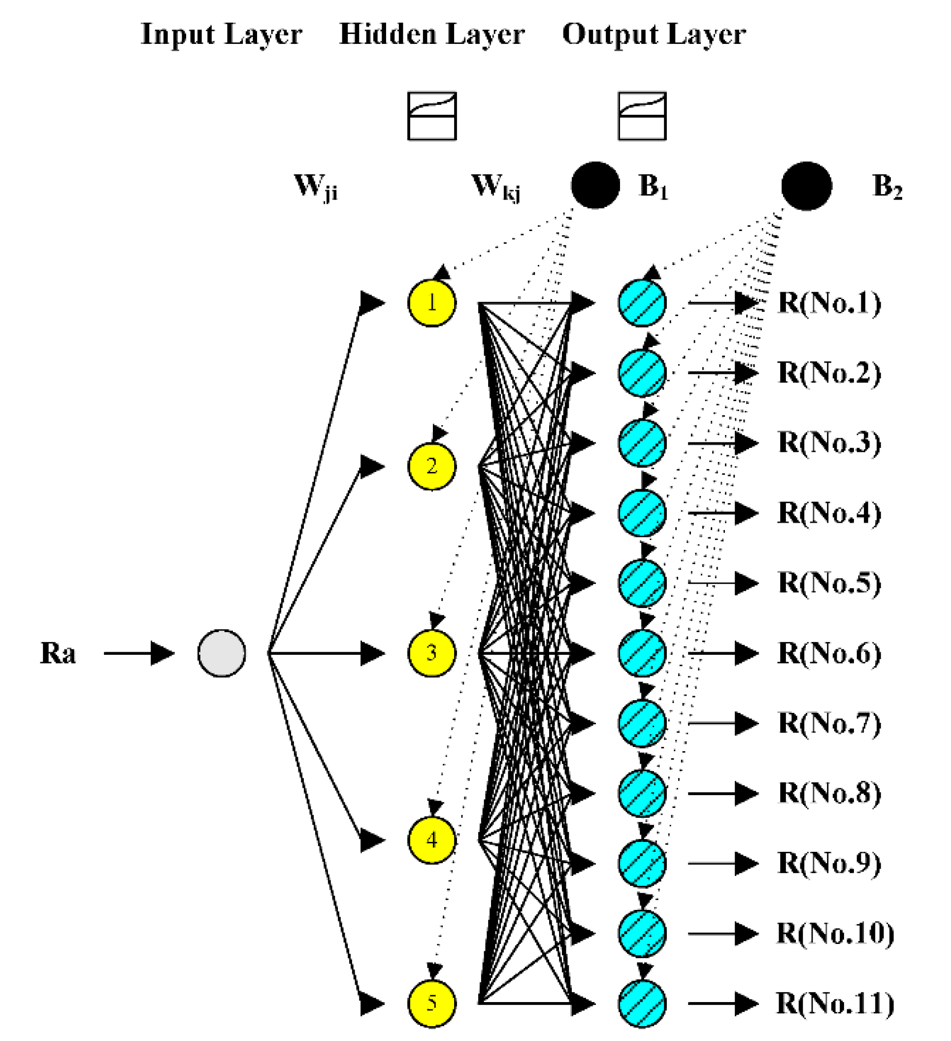
2.1. Multilayer Perceptron (MLP) Model

The MLP model has an input layer, an output layer, and one or more hidden layers between input and output layers. The nodes in one layer are connected only to the nodes of the immediate next layer. The strength of signal passing from one node to the other depends on the connection weights of interconnections. The hidden layers enhance the network’s ability to model complex functions.

The MLP model is trained using many kinds of backpropagation algorithms. Training is a process of adjusting the connection weights and biases, which calculate the error committed by the networks simply by taking the difference between the desired and actual responses, so that its output can match the desired output best [30,48]. Detailed information for the MLP model can be found in Tsoukalas and Uhrig [49] and Kim et al. [38,39,40].

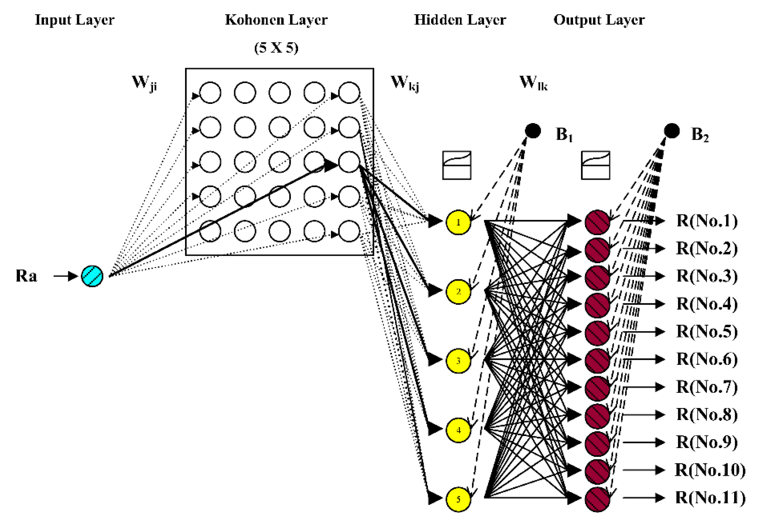
2.2. Kohonen Self-Organizing Feature Map (KSOFM) Model

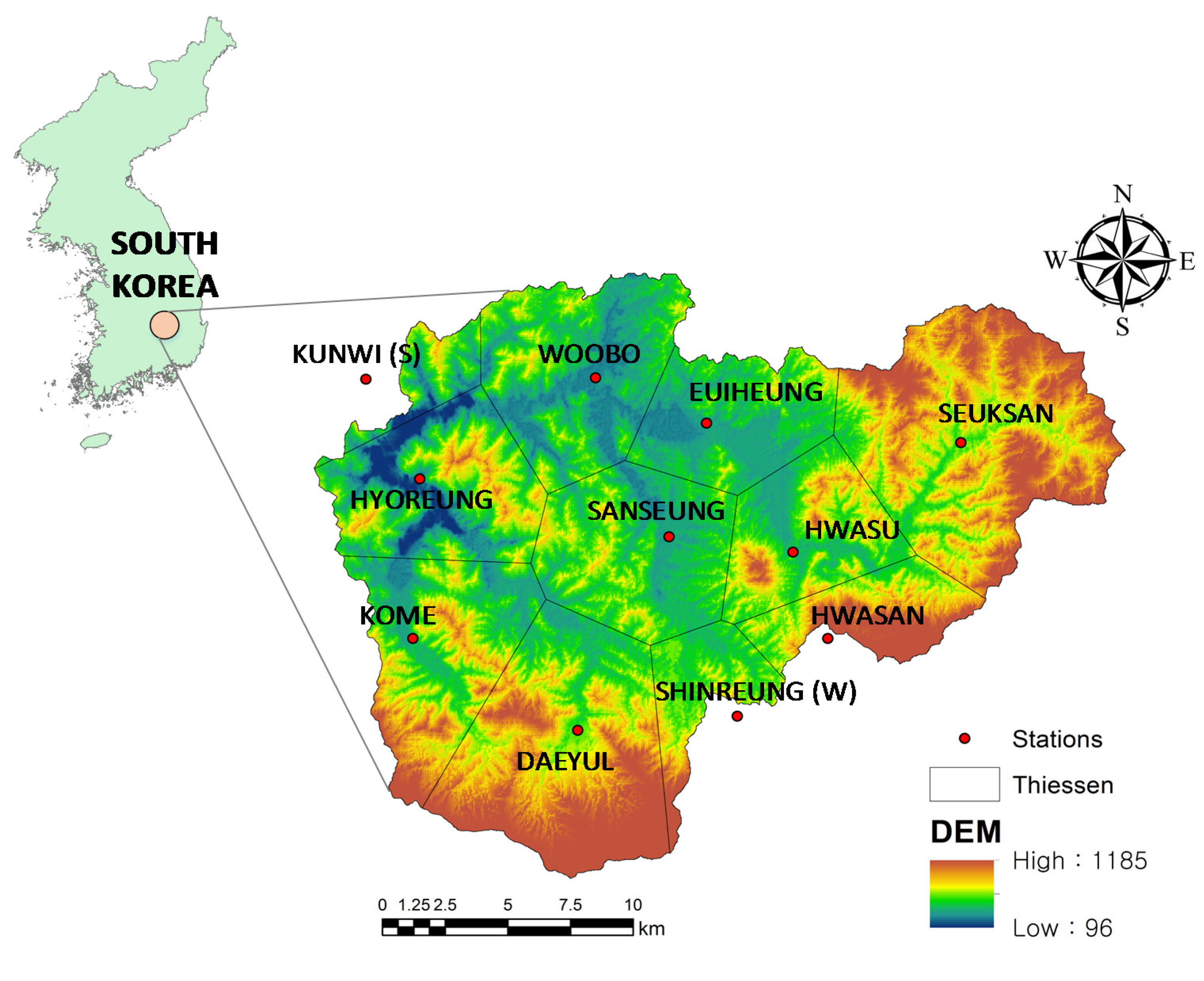
The KSOFM consists of four layers, that is, the input layer, Kohonen layer, hidden layer, and output layer. The input layer is composed of n input nodes, each connected to all nodes of the Kohonen layer [50,51,52,53,54]. The Kohonen layer consists of [n₁-by-n₁] matrices. The KSOFM model is a simple yet powerful learning process and an effective clustering method, and uses a neighborhood function to preserve the topological properties of the input space. It can transform high dimensional input patterns into the responses of two-dimensional arrays of neurons and perform this transformation adaptively in a topologically ordered fashion based on similarity. Detailed information on the KSOFM model can be found in Kohonen [55,56], Principe et al. [57], and Hsu et al. [58].

3. Case Study

The data derived from the Wi-stream catchment were employed to train, cross-validate, and test ANNs models. The Wi-stream catchment, shown in Figure 1, is located in 36°10′ N to 36°14′ N in latitude and in 128°33′ E to 128°54′ E in longitude. The catchment is in Kunwi-gun County, which is located in the center of Gyeongsangbuk-do province. The catchment, 472.53 km² in area, represents 77.1% of the total area, 612.86 km², of Kunwi-gun county. The Wi-stream catchment is narrow from south to north and long from east to west. The central part of the Wi-stream catchment is quite flat and suffers from storm and flood damages every year. There are six river stage stations, six groundwater stations, 11 rainfall stations, and 11 evaporation stations in the Wi-stream catchment. The stream network consists of one main stream and one tributary [59]. The hydrological data of the Wi-stream catchment, such as rainfall, river stage, discharge, and groundwater table, have been recorded since 1982.

Figure 1. Schematic diagram of the Wi-stream catchment.

Figure 1. Schematic diagram of the Wi-stream catchment.

To estimate areal rainfall using the kriging method in the Wi-stream catchment, hourly rainfall data from 11 rainfall stations, including Kunwi (S) (No.1), Hyoreung (No.2), Daeyul (No.3), Kome (No.4), Woobo (No.5), Sanseung (No.6), Shinreung (No.7), Euiheung (No.8), Hwasu (No.9), Hwasan (No.10), and Seuksan (No.11), were used. In order for ANNs to make accurate generalizations about rainfall, sufficient rainfall data should be available [31]. Rainfall must be recorded for more than 24 h, including non-rainfall hour, and non-rainfall period must be within 3 h in order to prevent overfitting when ANN models are trained for this study. Fourteen rainfall events (Cases 1–14) were chosen from the mid-1980s to the mid-1990s to meet this condition. For estimating areal rainfall using the MLP model, input nodes consist of point rainfall values from individual rainfall stations including Kunwi (S) (No.1), Hyoreung (No.2), Daeyul (No.3), Kome (No.4), Woobo (No.5), Sanseung (No.6), Shinreung (No.7), Euiheung (No.8), Hwasu (No.9), Hwasan (No.10), and Seuksan (No.11) stations. Output node consists of areal rainfall values using the kriging method from individual rainfall stations and vice versa for spatial disaggregation of areal rainfall using the MLP and KSOFM models.

For ANNs model, data were split into training, cross-validation, and testing sets. The training data were used for optimizing the connection weights and bias of ANNs model. In general, one of the problems that weaken the training performances is overfitting. If the overfitting problem occurs, the convergence process over the mean square error of the testing data will not decrease but will increase as the training data are still trained [31]. It usually occurs when an ANN model has memorized the training data and has not learned to generalize to new situations. To minimize the effect of overfitting, cross-validation data was used through an early stopping technique where an ANN model performance for the cross-validation data was monitored, and training performance was stopped when error on the cross-validation data began to rise. Once the ANN model was trained, the generalization and modeling ability of the ANN model was evaluated using a completely new testing data [60,61]. In all of these applications, 67% of data (Cases 1, 2, 3, 4, 5, 6, 7, 9 and 10, N = 338 h) was applied for training, 15% of data (Cases 8 and 11, N = 77 h) for cross-validation, and 18% of data (Cases 12, 13, and 14, N = 91 days) for testing.

Table 1 shows a summary of statistical indices of data used. In Table 1, X_mean, X_max, X_min, S_x, C_v, C_sx, and SE denote, respectively, the mean, maximum, minimum, standard deviation, coefficient of variation, skewness coefficient and standard error values of training, cross-validation, and testing data. The estimated values were compared with observed values using four different performance evaluation criteria: the Nash-Sutcliffe efficiency [62] (NS), root mean square error (RMSE), mean absolute error (MAE), and average performance error (APE). As a measure of the accuracy of any hydrologic model, NS is one of the most widely used criteria for calibration and evaluation of hydrological models [63]. It has been shown that NS alone cannot define which model is better than others. The various evaluation criteria (e.g., RMSE, MAE, and APE) must be used to define the model performance. The NS, RMSE, MAE, and APE evaluation criteria quantify the efficiency of a model in capturing extremely complex, dynamic, nonlinear, and fragmented relationships. A model, which is efficient in capturing the complex relationship among the various input and output variables involved in a particular problem, must be considered [64]. Table 2 shows mathematical expressions of performance evaluation criteria.

Table 1. Statistical indices of areal rainfall data using the kriging method.

Division	Number of Data	Statistical Indices of Areal Rainfall
		Xmean	Xmax	Xmin	Sx	Cv	Csx	SE
Training	338	3.26	27.76	0.00	4.21	1.12	2.32	0.21
Cross-validation	77	2.10	16.68	0.00	3.12	1.32	2.62	0.34
Testing	91	3.62	19.56	0.00	4.13	1.13	1.46	0.42

Table 1. Statistical indices of areal rainfall data using the kriging method.

Division	Number of Data	Statistical Indices of Areal Rainfall
		Xmean	Xmax	Xmin	Sx	Cv	Csx	SE
Training	338	3.26	27.76	0.00	4.21	1.12	2.32	0.21
Cross-validation	77	2.10	16.68	0.00	3.12	1.32	2.62	0.34
Testing	91	3.62	19.56	0.00	4.13	1.13	1.46	0.42

Table 2. Mathematical expressions of performance evaluation criteria.

Evaluation Criteria	Equation
NS	$\text{1}-\frac{{\displaystyle \sum _{\text{i}=\text{1}}^{\text{n}}{{\text{[y}}_{\text{i}}\text{(x)}-{\widehat{\mathrm{y}}}_i\text{(x)]}}^{\text{2}}}}{{\displaystyle \sum _{\text{i}=\text{1}}^{\text{n}}{{\text{[y}}_{\text{i}}\text{(x)}-{\text{u}}_{\text{y}}\text{]}}^{\text{2}}}}$
RMSE	$\sqrt{\frac{\text{1}}{\text{n}}{\displaystyle \sum _{\text{i}=\text{1}}^{\text{n}}{{\text{[y}}_{\text{i}}\text{(x)}-{\widehat{\mathrm{y}}}_{\mathrm{i}}\text{(x)]}}^{\text{2}}}}$
MAE	$\frac{\text{1}}{\text{n}}{\displaystyle \sum _{\mathrm{i}=1}^{\mathrm{n}}\left|{\mathrm{y}}_{\mathrm{i}}(x)-{\widehat{\mathrm{y}}}_{\mathrm{i}}(\mathrm{x})\right|}$
APE	$\frac{{\displaystyle \sum _{\text{i}=\text{1}}^{\text{n}}\left|{\text{y}}_{\text{i}}(\mathrm{x})-{\widehat{\mathrm{y}}}_{\mathrm{i}}(\mathrm{x})\right|}}{{\displaystyle \sum _{\text{i}=\text{1}}^{\text{n}}{\text{y}}_{\text{i}}\text{(x)}}}\times 100$

Notes: y_i (x) = the observed hourly rainfall (mm); y_i (x) = the estimated hourly rainfall (mm); u_v= the mean of observed hourly rainfall (mm); and n = the total number of hourly rainfall values considered.

Table 2. Mathematical expressions of performance evaluation criteria.

Evaluation Criteria	Equation
NS	$\text{1}-\frac{{\displaystyle \sum _{\text{i}=\text{1}}^{\text{n}}{{\text{[y}}_{\text{i}}\text{(x)}-{\widehat{\mathrm{y}}}_i\text{(x)]}}^{\text{2}}}}{{\displaystyle \sum _{\text{i}=\text{1}}^{\text{n}}{{\text{[y}}_{\text{i}}\text{(x)}-{\text{u}}_{\text{y}}\text{]}}^{\text{2}}}}$
RMSE	$\sqrt{\frac{\text{1}}{\text{n}}{\displaystyle \sum _{\text{i}=\text{1}}^{\text{n}}{{\text{[y}}_{\text{i}}\text{(x)}-{\widehat{\mathrm{y}}}_{\mathrm{i}}\text{(x)]}}^{\text{2}}}}$
MAE	$\frac{\text{1}}{\text{n}}{\displaystyle \sum _{\mathrm{i}=1}^{\mathrm{n}}\left|{\mathrm{y}}_{\mathrm{i}}(x)-{\widehat{\mathrm{y}}}_{\mathrm{i}}(\mathrm{x})\right|}$
APE	$\frac{{\displaystyle \sum _{\text{i}=\text{1}}^{\text{n}}\left|{\text{y}}_{\text{i}}(\mathrm{x})-{\widehat{\mathrm{y}}}_{\mathrm{i}}(\mathrm{x})\right|}}{{\displaystyle \sum _{\text{i}=\text{1}}^{\text{n}}{\text{y}}_{\text{i}}\text{(x)}}}\times 100$

Notes: y_i (x) = the observed hourly rainfall (mm); y_i (x) = the estimated hourly rainfall (mm); u_v= the mean of observed hourly rainfall (mm); and n = the total number of hourly rainfall values considered.

4. Applications and Results

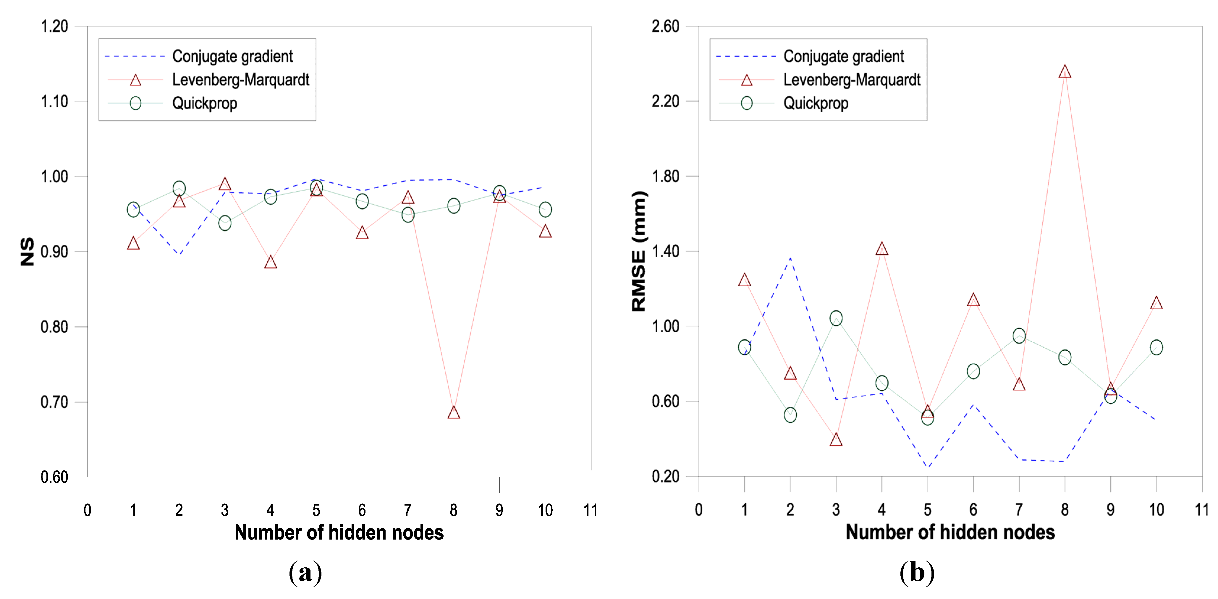
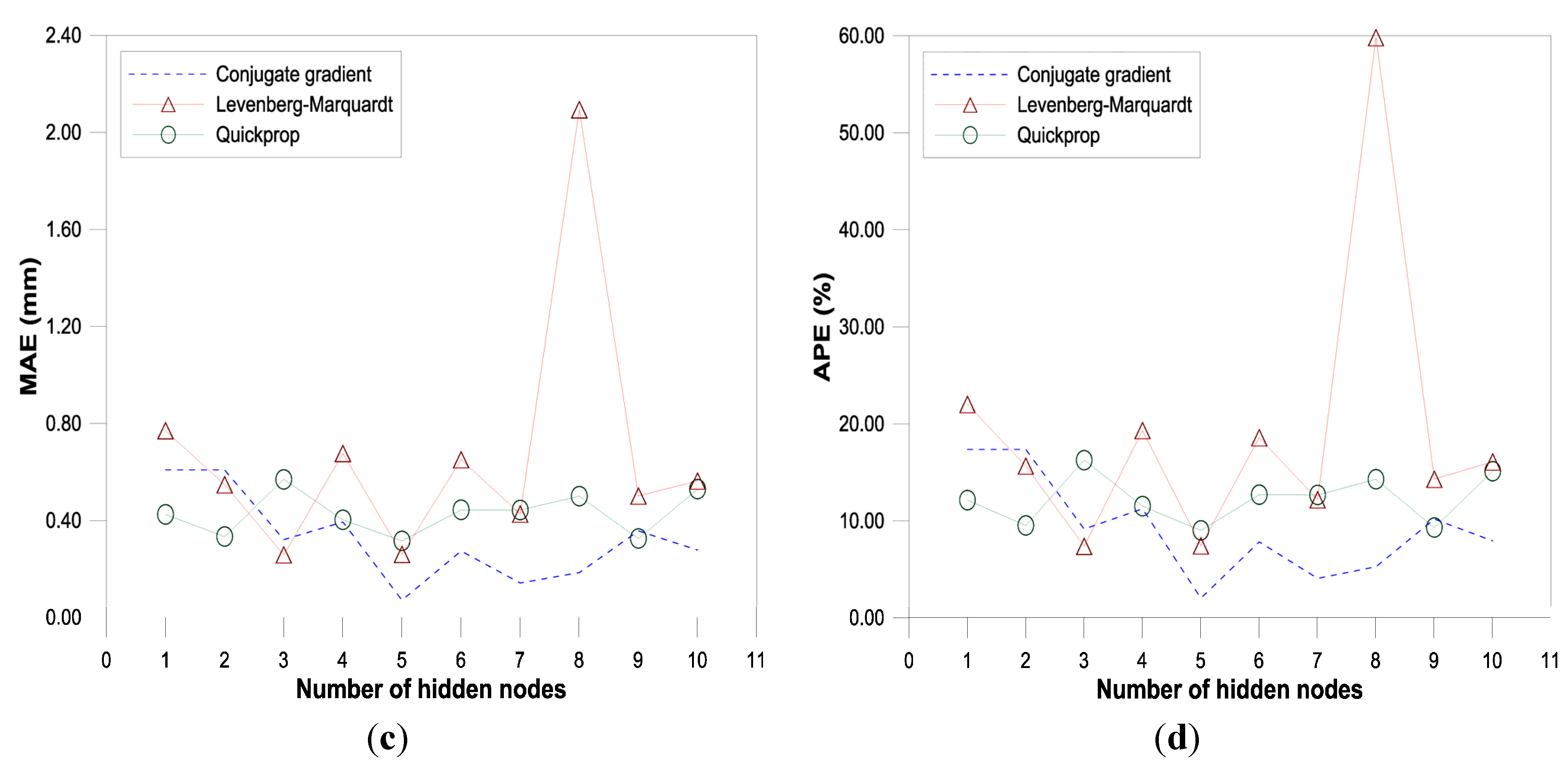
4.1. Selection of Optimal MLP Models for Estimating Areal Rainfall

Selection of an appropriate structure is important, because the network structure of ANNs directly affects the computational complexity and generalization capability [65]. Currently, there is no reliable and established method for selecting an appropriate network structure before completion of training [66]. A three-layer ANN, with a single hidden layer, has been usually sufficient for approximating conventional hydrological processes [67]. The training performance of ANNs is iterated until the training error is reached to the training tolerance [38,39,40]. In this study, the training tolerance where the mean square error converged to a certain value was fixed at 0.001. The training performances of MLP and KSOFM models were stopped after 10,000 iterations. Results of training were slightly different from each completion of training performance, because the values of initial weights for each layer were set as random values. Therefore, optimal parameters were determined when the results of training showed the best categories [31]. A three-layer MLP, with a single hidden layer, was used to estimate areal rainfall. Since the kriging method includes considerable variables to estimate the areal rainfall compared with the Thiessen polygon and spline methods, areal rainfall estimated using the kriging method was assumed as the observed areal rainfall. Based on the training data, the MLP model adopted three training algorithms, conjugate gradient [68,69], Levenberg–Marquardt [70,71], and quickprop [72], using different numbers of hidden nodes ranging from 1 to 10. Three training algorithms, including conjugate gradient, Levenberg–Marquardt, and quickprop, were used for the MLP model from the previous literatures. Outstanding results using the three training algorithms have been reported previously [37,38,39,40,41,42,43,44,61]. To overcome problems associated with extreme values, the data were normalized and scaled between 0 and 1. Another important reason for data normalization is that different data sets represent observed values in different units. The similarity effect of data was also eliminated [73,74].

Figure 2 shows the influence of the number of hidden nodes on the performance evaluation criteria (NS, RMSE, MAE, and APE) for three training algorithms during the test period. The Levenberg-Marquardt training algorithm was more sensitive to the number of hidden nodes than were conjugate gradient and quickprop training algorithms, as seen from large fluctuations with respect to the number of hidden nodes. This result is consistent with that reported by [61]. The best values of NS, RMSE, MAE, and APE for 11-5-1 networks were, respectively, 0.996, 0.242, 0.072, and 2.014 for the conjugate gradient training algorithm. The best values of NS, RMSE, MAE, and APE for 11-3-1 networks were, respectively, 0.992, 0.398, 0.258, and 7.401 for the Levenberg-Marquardt training algorithm. The best values of NS, RMSE, MAE, and APE for 11-5-1 networks were, respectively, 0.984, 0.514, 0.317, and 9.029 for quickprop training algorithm. It is clear from Figure 2a–d that 11-5-1 networks was the best for conjugate gradient and quickprop training algorithms, and 11-3-1 networks was the best for Levenberg-Marquardt training algorithm. The inverse networks of 11-5-1 and 11-3-1 structures, 1-5-11 (conjugate gradient and quickprop) and 1-3-11 (Levenberg-Marquardt), were identified for spatial disaggregation of areal rainfall using the MLP model. In this study, results of the MLP output layer with a 11-5-1 structure can be written as:

$${\text{R}}_{\mathrm{a}}{\text{=Φ}}_{\text{2}}\text{(}{\displaystyle \sum _{\text{k}=\text{1}}^{\text{1}}{\text{W}}_{\text{kj}}\cdot {\text{Φ}}_{\text{1}}\text{(}{\displaystyle \sum _{\text{j}=\text{1}}^5{\text{W}}_{\text{ji}}\cdot \text{X(t)}+{\text{B}}_{\text{1}}\text{)}+{\text{B}}_{\text{2}}\text{)}}}$$

(1)

where i, j, k = the input, hidden, and output layers, respectively; ${\text{R}}_{\mathrm{a}}$ = the areal rainfall (mm); ${\text{Φ}}_{\text{1}}\text{(}\cdot \text{)}$ = the linear sigmoid transfer function of hidden layer; ${\text{Φ}}_{\text{2}}\text{(}\cdot \text{)}$ = the linear sigmoid transfer function of output layer; W_kj = the connection weights between the hidden and output layers; W_ji = the connection weights between the input and hidden layers; $\text{X(t)}$ = the time series data of input variables; ${\text{B}}_{\text{1}}$ = the bias in hidden layer; and ${\text{B}}_{\text{2}}$ = the bias in output layer. Figure 3 shows the structure of MLP (11-5-1) developed for estimating areal rainfall in this study.

Figure 2. Influence of the number of hidden nodes for three training algorithms (test period). (a) NS; (b) MAF; (c) RMSE; (d) APE.

Figure 2. Influence of the number of hidden nodes for three training algorithms (test period). (a) NS; (b) MAF; (c) RMSE; (d) APE.

Figure 3. Structure of MLP (11-5-1) developed for estimating areal rainfall.

Figure 3. Structure of MLP (11-5-1) developed for estimating areal rainfall.

Before the chosen structures, such as 11-5-1 and 11-3-1, for three training algorithms were used for the spatial disaggregation of areal rainfall, homogeneity between observed (kriging method) and estimated (MLP model) areal rainfall values was analyzed. The Mann-Whitney U test, one of the tests for homogeneity, was used to compare observed and estimated areal rainfall values to evaluate the confidence level of MLP model. It is a nonparametric alternative to the two-sample t-test for two independent samples and can be used to test whether two independent samples have been taken from the same population [75,76,77,78]. The critical value of z statistic (z_α) was computed for the specific level of significance. If the computed value of z statistic is greater than the critical value of z statistic (z_α), the null hypothesis, that the two independent samples are from the same population, should be rejected and the alternative hypothesis should be accepted.

Table 3 shows results of the Mann-Whitney U test between observed and estimated areal rainfall values for the testing data. The critical value of z statistic (z_α), z_0.05 = 1.960, was computed for the five percent level of significance. Since the computed values of z statistic for both stations were not significant, the null hypothesis was accepted for areal rainfall using the MLP model.

Table 3. Results of the Mann-Whitney U test.

Model	Networks	Training Algorithms	Level of Significance	Mann-Whitney U test
				Critical z Statistic	Computed z Statistic	Null Hypothesis
MLP	11-5-1	Conjugate gradient	0.05	1.960	−0.287	Accept
	11-3-1	Levenberg–Marquardt	0.05	1.960	−0.617	Accept
	11-5-1	Quickprop	0.05	1.960	−0.515	Accept

Table 3. Results of the Mann-Whitney U test.

Model	Networks	Training Algorithms	Level of Significance	Mann-Whitney U test
				Critical z Statistic	Computed z Statistic	Null Hypothesis
MLP	11-5-1	Conjugate gradient	0.05	1.960	−0.287	Accept
	11-3-1	Levenberg–Marquardt	0.05	1.960	−0.617	Accept
	11-5-1	Quickprop	0.05	1.960	−0.515	Accept

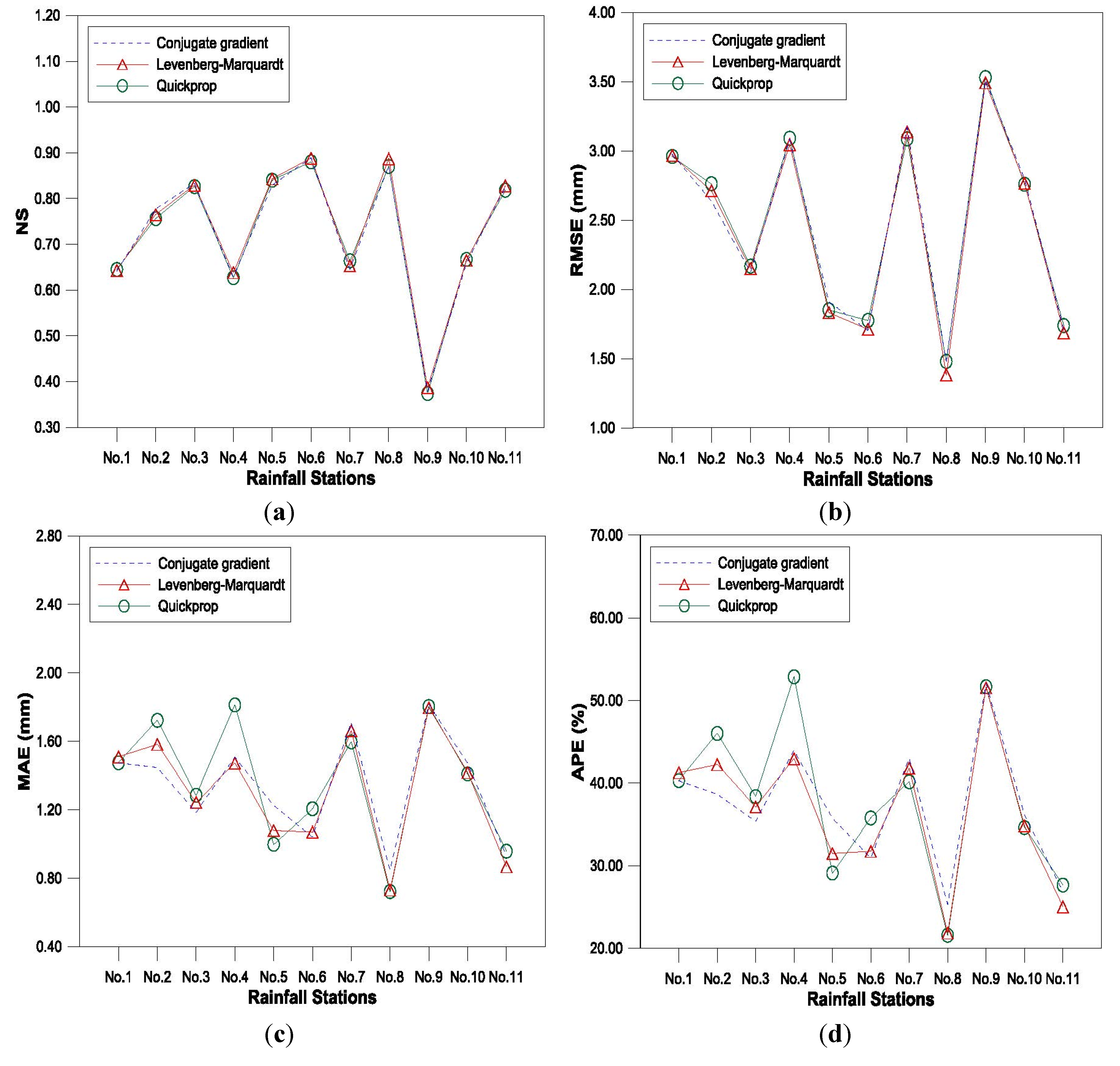
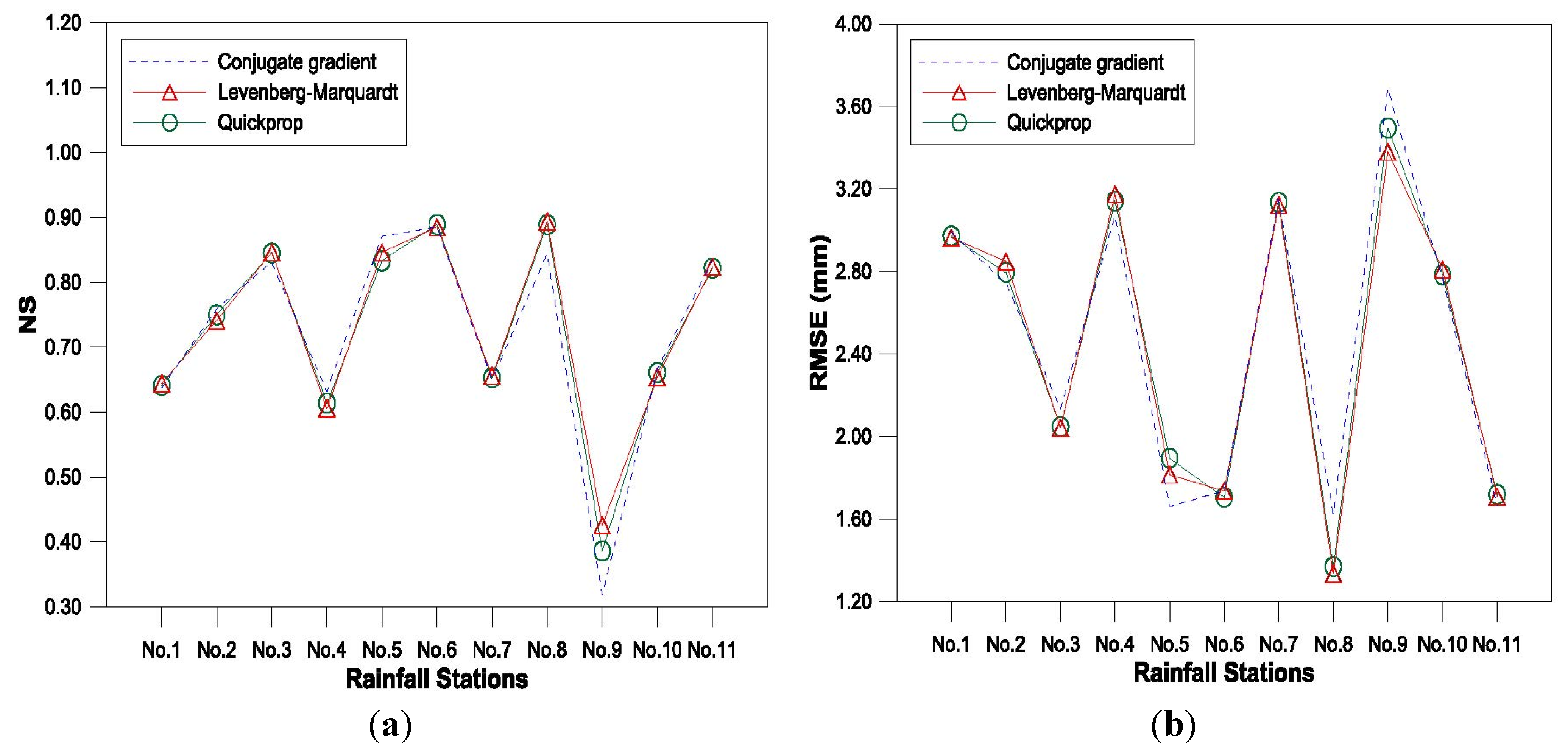
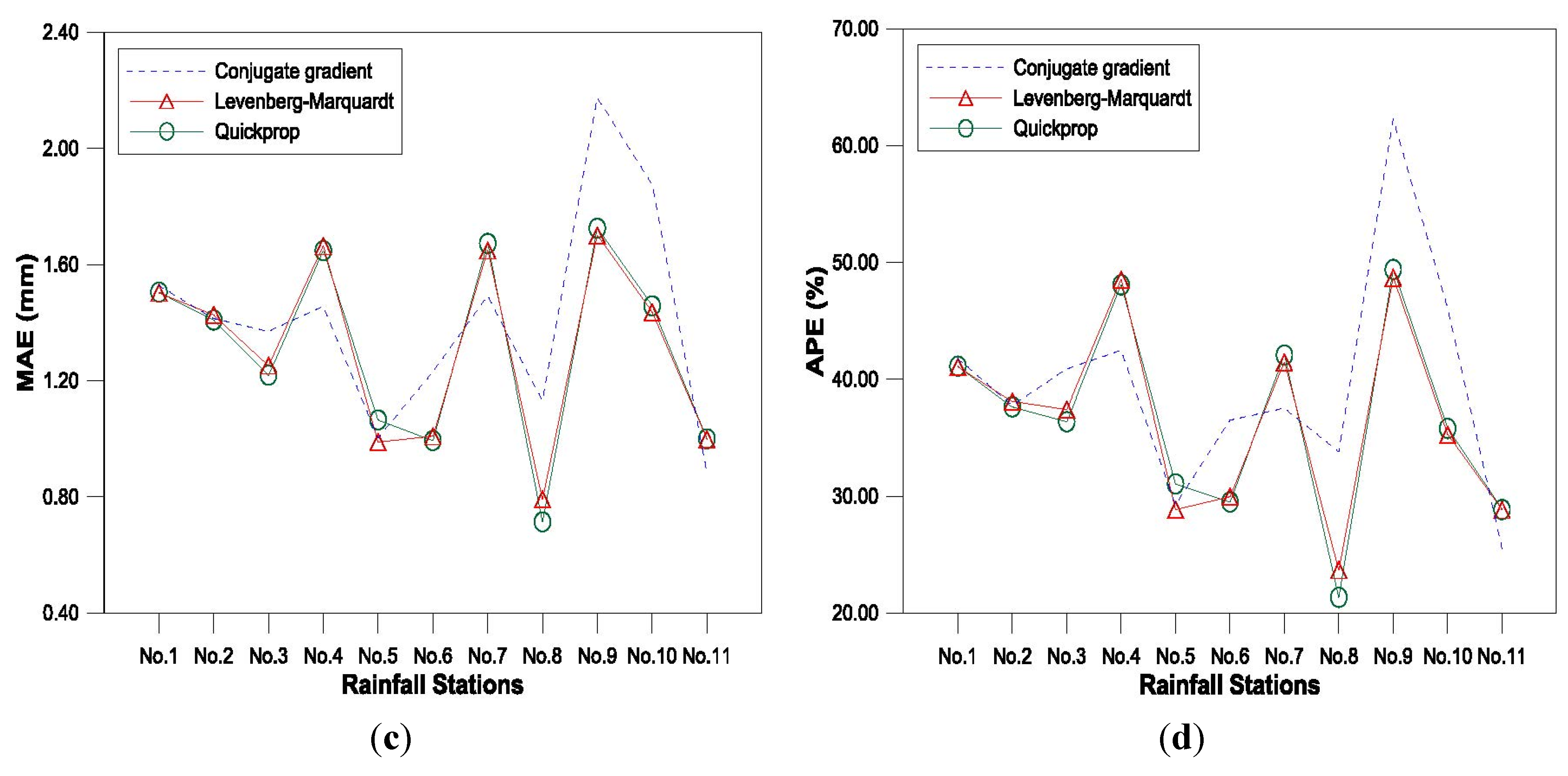
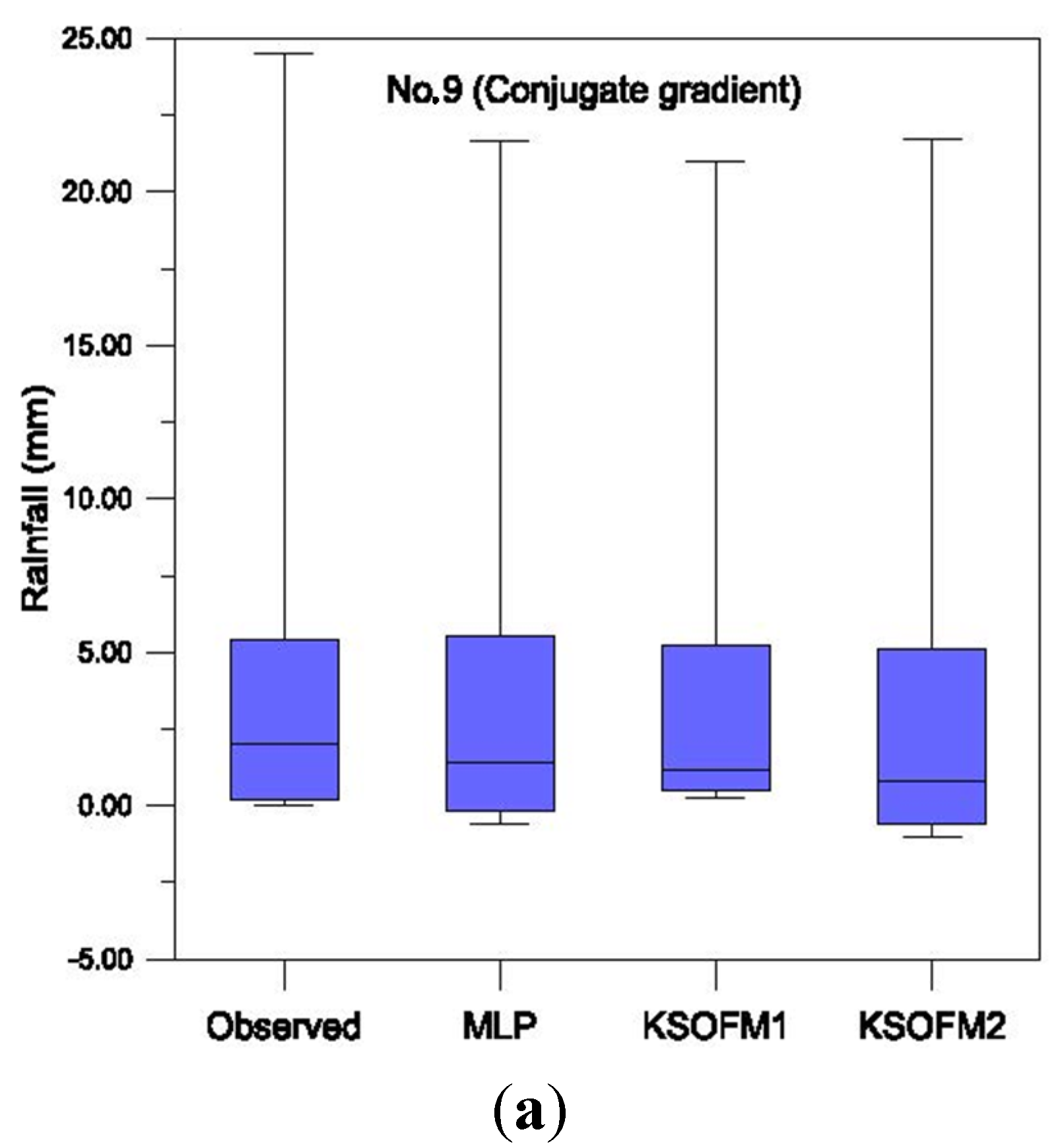
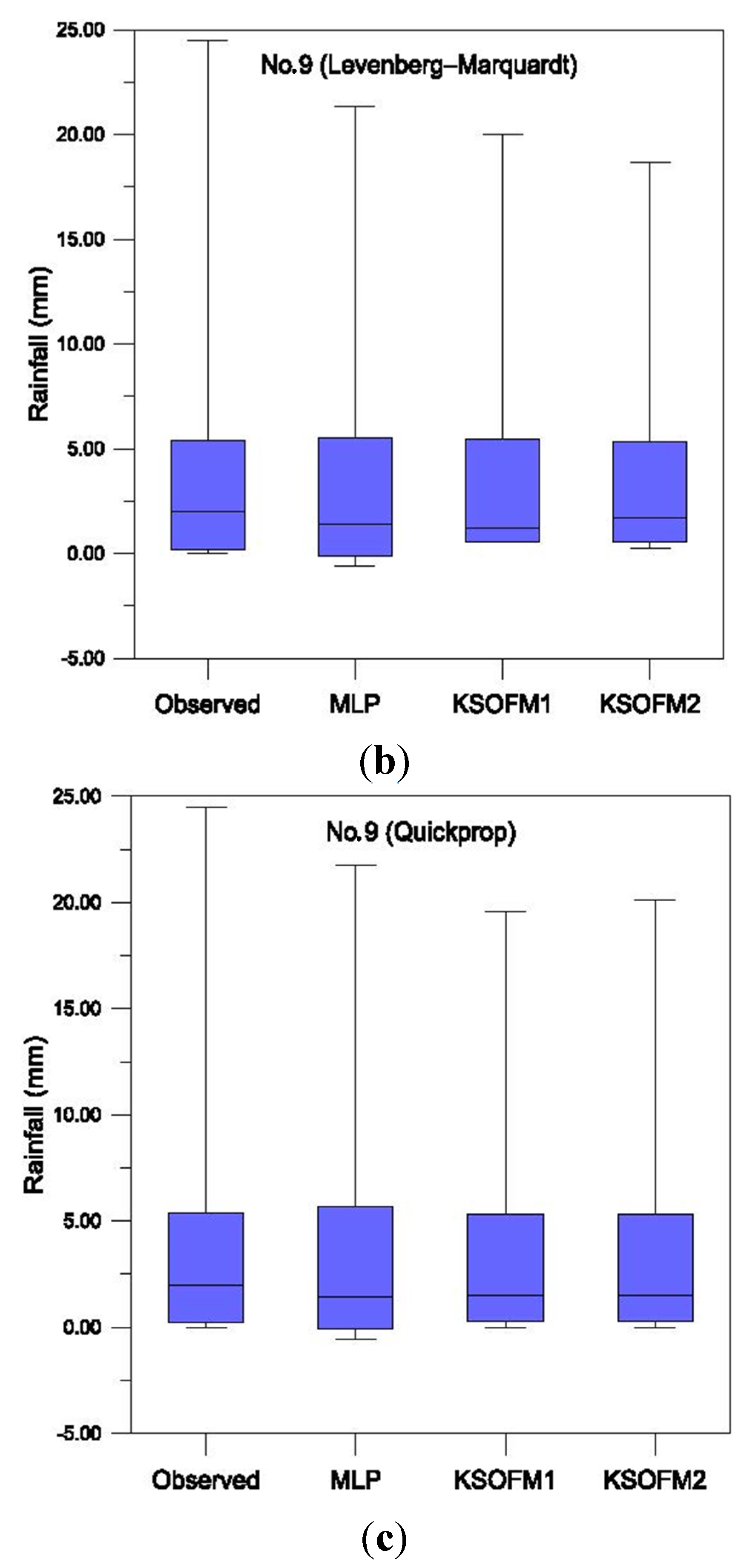
4.2. Evaluation for Spatial Disaggregation of Areal Rainfall Using MLP Model

Three different MLP models, including 1-5-11 (conjugate gradient), 1-3-11 (Levenberg–Marquardt), and 1-5-11 (quickprop), were used for spatial disaggregation of areal rainfall. Figure 4 shows the developed structure of MLP (1-5-11) for spatial disaggregation of areal rainfall.

Figure 4. Structure of MLP (1-5-11) developed for spatial disaggregation of areal rainfall.

Figure 4. Structure of MLP (1-5-11) developed for spatial disaggregation of areal rainfall.

Figure 5 shows the influence of individual rainfall station on the performance evaluation criteria (NS, RMSE, MAE, and APE) for three training algorithms during the test period. The three training algorithms were generally sensitive to individual rainfall station, as seen from large fluctuations with respect to the individual rainfall station. The spatial disaggregated rainfall using three training algorithms yielded similar values on the performance evaluation criteria (NS, RMSE, MAE, and APE) for individual rainfall station. For Euiheung (No.8) station, the values of NS, RMSE, MAE, and APE were 0.870, 1.480, 0.849, and 25.335, respectively, for 1-5-11 structure (conjugate gradient); were 0.886, 1.385, 0.732, and 21.863, respectively, for 1-3-11 structure (Levenberg–Marquardt); and were 0.869, 1.481, 0.723, and 21.553, respectively, for 1-5-11 structure (quickprop). Figure 5a–d shows that spatial disaggregated rainfall at Euiheung (No.8) station yielded the best results among the 11 rainfall stations for the MLP model. For Hwasu (No.9) station, the values of NS, RMSE, MAE, and APE were 0.378, 3.515, 1.817, and 52.021, respectively, for 1-5-11 structure (conjugate gradient); were 0.388, 3.492, 1.795, and 51.431, respectively, for 1-3-11 structure (Levenberg–Marquardt); and were 0.373, 3.531, 1.805, and 51.680, respectively, for 1-5-11 structure (quickprop). Figure 5a–d shows that spatial disaggregated rainfall at Hwasu (No.9) station yielded the worst results among the 11 rainfall stations for the MLP model. In this study, the MLP model is capable of disaggregating areal rainfall into individual point rainfall.

Figure 5. Influence of individual rainfall stations for three training algorithms of MLP (test period). (a) NS; (b) MAF; (c) RMSE; (d) APE.

Figure 5. Influence of individual rainfall stations for three training algorithms of MLP (test period). (a) NS; (b) MAF; (c) RMSE; (d) APE.

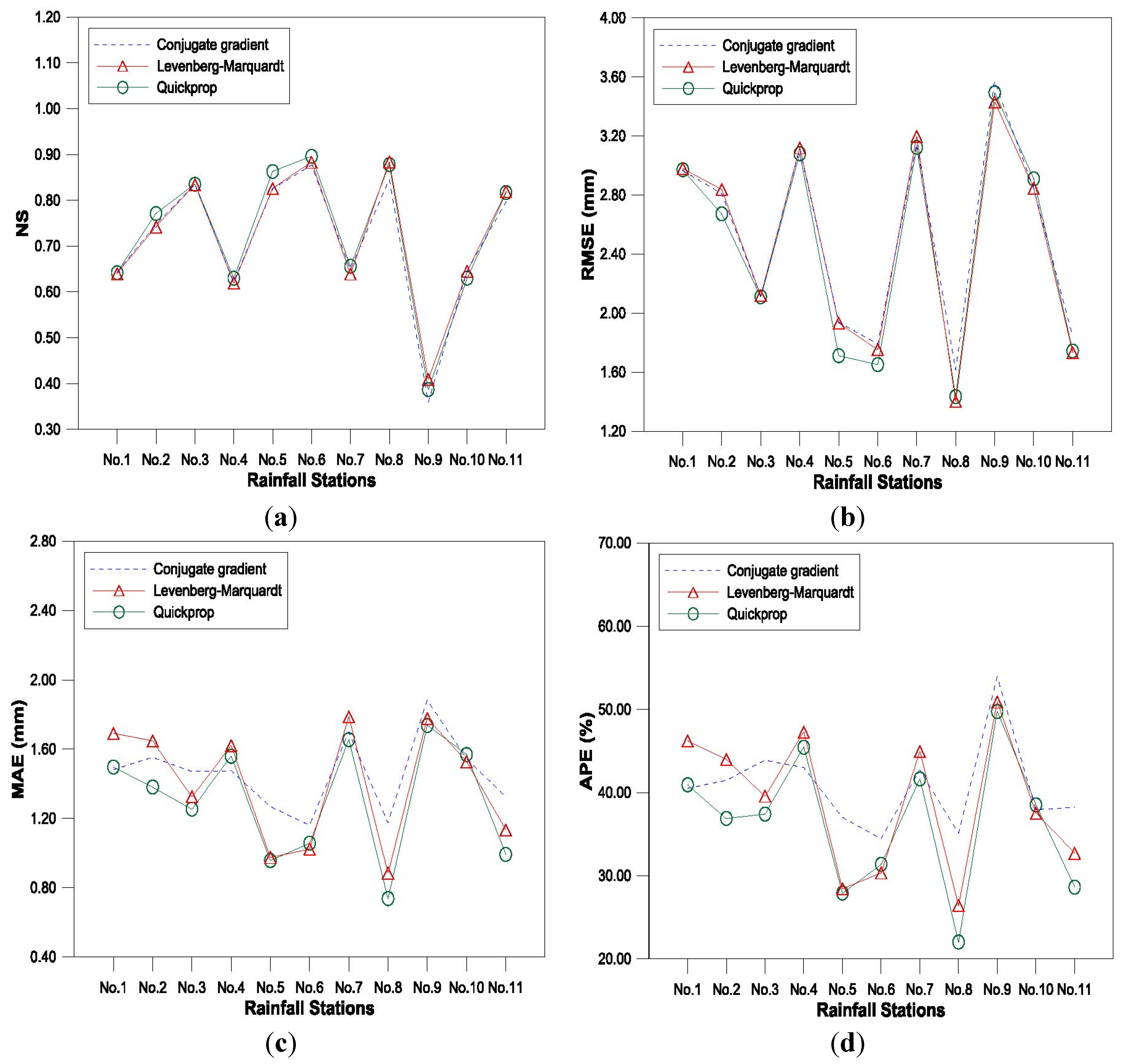
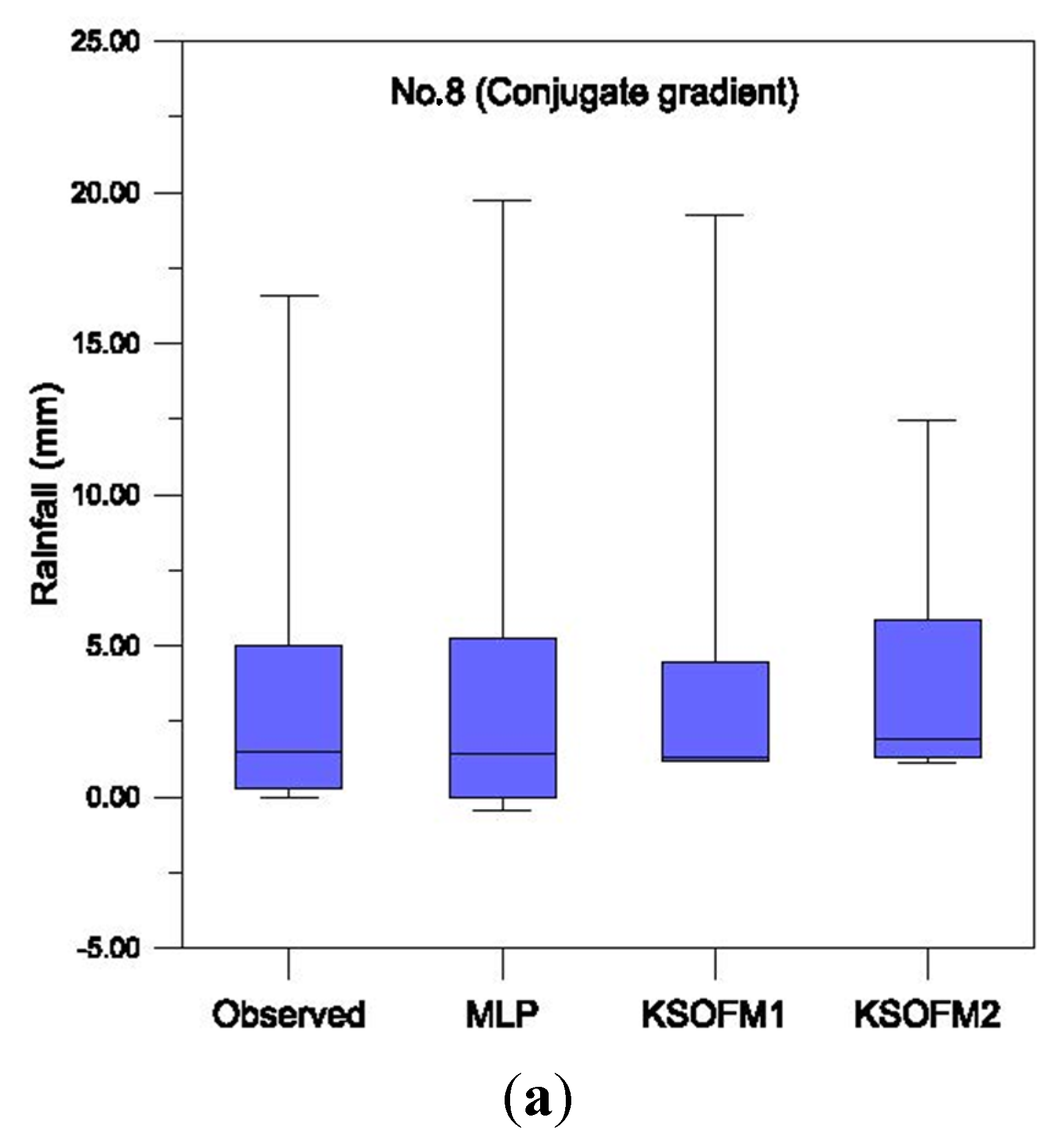
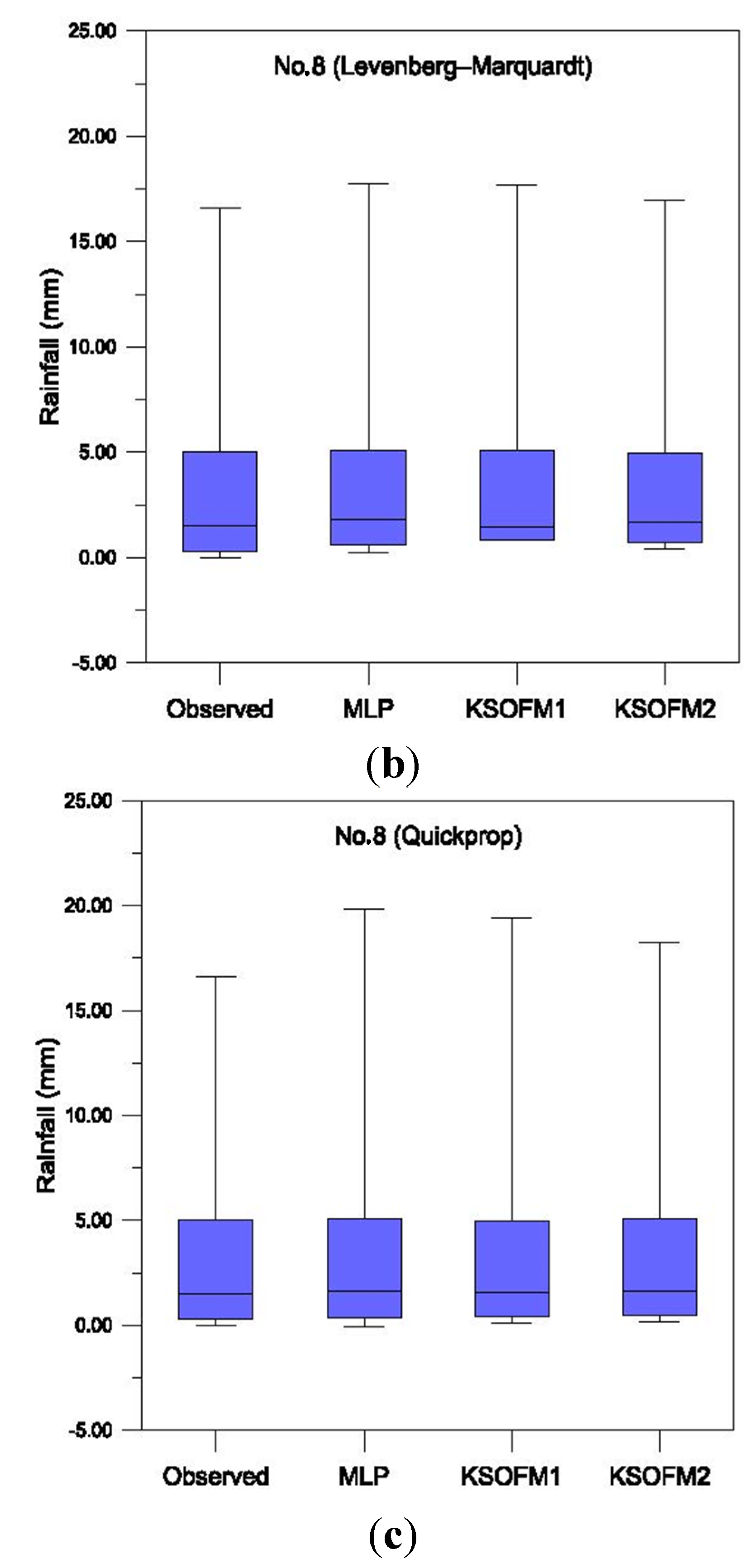
4.3. Evaluation for Spatial Disaggregation of Areal Rainfall Using KSOFM Model

The KSOFM model was used and compared with the MLP model for spatial disaggregation of areal rainfall. The KSOFM model classifies each input node and determines as to which node in the hidden layer it must be routed for spatial disaggregation of areal rainfall for the output layer. Six different KSOFM models, including (1) [5-by-5] and [7-by-7] matrices in the Kohonen layer; and (2) 11-5-1 (conjugate gradient), 11-3-1 (Levenberg–Marquardt), and 11-5-1 (quickprop) in the hidden layer, were used for spatial disaggregation of areal rainfall. Figure 6 shows the developed structure of the KSOFM (1-[5-by-5]-5-11) for spatial disaggregation of areal rainfall. Results of the KSOFM output layer with 1-[5-by-5]-5-11 structure can be written as:

$${\mathrm{R}}_{\mathrm{d}}{\text{=Φ}}_{\text{2}}\text{(}{\displaystyle \sum _{\text{l}=\text{1}}^{\text{11}}{\text{W}}_{\text{lk}}\cdot }{\text{Φ}}_{\text{1}}\text{(}{\displaystyle \sum _{\text{k}=\text{1}}^5{\text{W}}_{\text{kj}}\cdot {\text{S}}_{\text{j}}}+{\text{B}}_{\text{1}}\text{)}+{\text{B}}_{\text{2}}\text{)}$$

(2)

where i, j, k, l = the input, Kohonen, hidden, and output layers, respectively; ${\text{R}}_{\mathrm{d}}$ = the disaggregated rainfall (mm) for individual rainfall station; W_kj = the connection weights between the Kohonen and hidden layers; S_j = the results calculated from the Euclidean distance (d_j) and the Kohonen layer; ${\text{Φ}}_1(\cdot )$ = the linear sigmoid transfer function of hidden layer; ${\text{Φ}}_2(\cdot )$ = the linear sigmoid transfer function of output layer; B₁ = the bias in hidden layer; B₂ = the bias in output layer; and W_lk = the connection weights between the hidden and output layers. The Euclidean distance between the input and Kohonen nodes can be written as:

$${\mathrm{d}}_{\mathrm{j}}=\sqrt{{\displaystyle \sum _{\mathrm{i}=1}^{\mathrm{n}}{({\mathrm{x}}_{\mathrm{i}}-{\mathrm{W}}_{\mathrm{j}\mathrm{i}})}^2}}$$

(3)

Figure 6. Structure of KSOFM (1-[5 X 5]-5-11) developed for spatial disaggregation of areal rainfall.

Figure 6. Structure of KSOFM (1-[5 X 5]-5-11) developed for spatial disaggregation of areal rainfall.

Figure 7 shows the influence of individual rainfall station on the performance evaluation criteria (NS, RMSE, MAE, and APE) for the three training algorithms of the KSOFM model based on [5-by-5] matrice (KSOFM1) during the test period. The three training algorithms were generally sensitive to individual rainfall station, as seen from large fluctuations with respect to the individual rainfall station. The spatial disaggregated rainfall using the three training algorithms yielded similar values on the performance evaluation criteria (NS, RMSE, MAE, and APE) for individual rainfall station. For Euiheung (No.8) station, the values of NS, RMSE, MAE, and APE were 0.847, 1.615, 1.174, and 35.129, respectively, for 1-5-11 structure (conjugate gradient); were 0.885, 1.402, 0.884, and 26.462, respectively, for 1-3-11 structure (Levenberg–Marquardt); and were 0.877, 1.436, 0.738, and 22.035, respectively, for 1-5-11 structure (quickprop). Figure 7 shows that spatial disaggregated rainfall at Euiheung (No.8) station yielded the best results among the 11 rainfall stations for KSOFM1 model. For Hwasu (No.9) station, the values of NS, RMSE, MAE, and APE were 0.358, 3.573, 1.885, and 53.953, respectively, for 1-5-11 structure (conjugate gradient); were 0.408, 3.432, 1.778, and 50.907, respectively, for 1-3-11 structure (Levenberg–Marquardt); and were 0.388, 3.492, 1.736, and 49.732, respectively, for 1-5-11 structure (quickprop). Figure 7 shows that spatial disaggregated rainfall at Hwasu (No.9) station yielded the worst results among the 11 rainfall stations for KSOFM1 model.

Figure 7. Influence of individual rainfall stations for three training algorithms of KSOFM1 (test period). (a) NS; (b) MAF; (c) RMSE; (d) APE.

Figure 7. Influence of individual rainfall stations for three training algorithms of KSOFM1 (test period). (a) NS; (b) MAF; (c) RMSE; (d) APE.

Figure 8 shows the influence of individual rainfall station on the performance evaluation criteria (NS, RMSE, MAE, and APE) for the three training algorithms of the KSOFM model based on [7-by-7] matrice (KSOFM2) during the test period. The three training algorithms were generally sensitive to individual rainfall station, as seen from large fluctuations with respect to the individual rainfall station. The spatial disaggregated rainfall using three training algorithms yielded similar values on performance evaluation criteria (NS, RMSE, MAE, and APE) for individual rainfall station. For Euiheung (No.8) station, the values of NS, RMSE, MAE, and APE were 0.845, 1.622, 1.130, and 33.806, respectively, for 1-5-11 structure (conjugate gradient); were 0.895, 1.334, 0.791, and 23.680, respectively, for 1-3-11 structure (Levenberg–Marquardt); and were 0.888, 1.371, 0.715, and 21.354, respectively, for 1-5-11 structure (quickprop). Figure 8 shows that spatial disaggregated rainfall at Euiheung (No.8) station yielded the best results among the 11 rainfall stations for the KSOFM2 model. For Hwasu (No.9) station, the values of NS, RMSE, MAE, and APE were 0.317, 3.687, 2.176, and 62.290, respectively, for 1-5-11 structure (conjugate gradient); were 0.427, 3.378, 1.702, and 48.680, respectively, for 1-3-11 structure (Levenberg–Marquardt); and were 0.385, 3.496, 1.726, and 49.398, respectively, for 1-5-11 structure (quickprop). Figure 8 shows that spatial disaggregated rainfall at Hwasu (No.9) station yielded the worst results among the 11 rainfall stations for the KSOFM2 model. In this study, the KSOFM1 and KSOFM2 models were capable of disaggregating areal rainfall into individual point rainfall. However, because of strong nonlinearity of rainfall, it is difficult to conclude with confidence which model is superior to other models. The specific rainfall stations did not generally show the satisfactory results in the evaluation criteria for the three training algorithms of the MLP, KSOFM1, and KSOFM2 performances. It can be found that the spatial distribution of rainfall stations can affect the performance of ANNs models from this observation.

Figure 8. Influence of individual rainfall stations for three training algorithms of KSOFM2 (test period). (a) NS; (b) MAF; (c) RMSE; (d) APE.

Figure 8. Influence of individual rainfall stations for three training algorithms of KSOFM2 (test period). (a) NS; (b) MAF; (c) RMSE; (d) APE.

Figure 9 and Figure 10 show the box plots for spatial disaggregated rainfall during the test period at Euiheung (No.8) and Hwasu (No.9) stations. The box plots show the distributions of basic statistics for performances of MLP, KSOFM1, and KSOFM2 with three training algorithms. Figure 9 and Figure 10 show the centerline (median) dividing the rectangular box defined by 25th and 75th percentiles, and lines extend from maximum to minimum data point at Euiheung (No.8) and Hwasu (No.9) stations. The basic statistics of spatial disaggregated rainfall for performances of the MLP, KSOFM1, and KSOFM2 models yielded similar behaviors compared with observed rainfall at Euiheung (No.8) and Hwasu (No.9) stations except for the maximum rainfall values.

Figure 9. Rainfall box plots for Euiheung (No.8) station (test period). (a) Conjugate gradient; (b) Levenberg–Marquardt; (c) Quickprop.

Figure 9. Rainfall box plots for Euiheung (No.8) station (test period). (a) Conjugate gradient; (b) Levenberg–Marquardt; (c) Quickprop.

Figure 10. Rainfall box plots for Hwasu (No.9) station (test period). (a) Conjugate gradient; (b) Levenberg–Marquardt; (c) Quickprop.

Figure 10. Rainfall box plots for Hwasu (No.9) station (test period). (a) Conjugate gradient; (b) Levenberg–Marquardt; (c) Quickprop.

5. Conclusions

This study develops and evaluates artificial neural network (ANN) models for spatial disaggregation of areal rainfall in the Wi-stream catchment, an IHP representative catchment, in South Korea. A three-layer MLP is used to estimate areal rainfall. Areal rainfall estimated using the kriging method is assumed as observed areal rainfall. Based on training data, the MLP models employ three training algorithms, conjugate gradient, Levenberg–Marquardt, and quickprop.

The influence of number of hidden nodes for the three training algorithms is evaluated to estimate areal rainfall using the MLP model. The Levenberg-Marquardt training algorithm is more sensitive to the number of hidden nodes than are the conjugate gradient and quickprop training algorithms. It is seen from large fluctuations with respect to the number of hidden nodes. The Mann-Whitney U test is performed to compare observed and estimated areal rainfall values to evaluate the confidence level of the MLP model. The null hypothesis is accepted for areal rainfall using the MLP model. The structures of 1-5-11 (conjugate gradient and quickprop) and 1-3-11 (Levenberg–Marquardt) are identified for spatial disaggregation of areal rainfall using the MLP model.

Three different MLP models are employed for spatial disaggregation of areal rainfall. The influence of individual rainfall station to disaggregate areal rainfall using the MLP model is evaluated. Three training algorithms are generally sensitive to individual rainfall station, as seen from large fluctuations with respect to the individual rainfall station. The spatial disaggregated rainfall using the three training algorithms yields similar values for individual rainfall station. The spatial disaggregated rainfall at Euiheung (No.8) station yields the best results, whereas spatial disaggregated rainfall at Hwasu (No.9) station yields the worst results among the 11 rainfall stations using the MLP model.

The KSOFM model is compared with the MLP model for spatial disaggregation of areal rainfall. Six different KSOFM models are employed for spatial disaggregation of areal rainfall. The spatial disaggregated rainfall at Euiheung (No.8) station yields the best results, whereas spatial disaggregated rainfall at Hwasu (No.9) station yields the worst results among the 11 rainfall stations using the KSOFM1 and KSOFM2 models, respectively.

It can be found that the MLP, KSOFM1, and KSOFM2 models can disaggregate areal rainfall into individual point rainfall. However, because of strong nonlinearity of rainfall, it is difficult to conclude with confidence as to which model is superior. Continuing studies, including data extension and new model application, are needed for aggregation and disaggregation of rainfall.

References

1. Burian, S.J.; Durrans, S.R.; Tomić, S.; Pimmel, R.L.; Wai, C.N. Rainfall disaggregation using artificial neural networks. J. Hydrol. Eng. ASCE 2000, 5, 299–307. [Google Scholar] [CrossRef]
2. Boushaki, F.I.; Hsu, K.L.; Sorooshian, S.; Park, G.H.; Mahani, S.; Shi, W. Bias adjustment of satellite precipitation estimation using ground-based measurement: A case study evaluation over the southwestern United States. J. Hydrometeor. 2009, 10, 1231–1242. [Google Scholar] [CrossRef]
3. AghaKouchak, A.; Bárdossy, A.; Habib, E. Conditional simulation of remotely sensed rainfall data using a non-Gaussian v-transformed copula. Adv. Water Resour. 2010, 33, 624–634. [Google Scholar] [CrossRef]
4. Chow, V.T.; Maidment, D.R.; Mays, L.W. Applied Hydrology; McGraw-Hill: New York, NY, USA, 1988. [Google Scholar]
5. Goovaerts, P. Geostatistical approaches for incorporating elevation into the spatial interpolation of rainfall. J. Hydrol. 2000, 228, 113–129. [Google Scholar] [CrossRef]
6. Singh, V.P. Elementary Hydrology; Prentice Hall: Englewood Cliffs, NJ, USA, 1992. [Google Scholar]
7. Apaydin, H.; Sonmez, F.K.; Yildirim, Y.E. Spatial interpolation techniques for climate data in the GAP region in Turkey. Clim. Res. 2004, 28, 31–40. [Google Scholar] [CrossRef]
8. Tait, A.; Henderson, R.; Turner, R.; Zheng, X. Thin plate smoothing spline interpolation of daily rainfall for New Zealand using a climatological rainfall surface. Int. J. Climatol. 2006, 26, 2097–2115. [Google Scholar] [CrossRef]
9. Ly, S.; Charles, C.; Degré, A. Geostatistical interpolation of daily rainfall at catchment scale: The use of several variogram models in the Ourthe and Ambleve catchments, Belgium. Hydrol. Earth Syst. Sci. 2011, 15, 2259–2274. [Google Scholar] [CrossRef]
10. Genest, C.; Favre, A.; Béliveau, J.; Jacques, C. Metaelliptical copulas and their use in frequency analysis of multivariate hydrological data. Water Resour. Res. 2007, 43, W09401:1–W09401:12. [Google Scholar] [CrossRef]
11. Zhang, L.; Singh, V.P. Bivariate rainfall frequency distributions using Archimedean copulas. J. Hydrol. 2007, 332, 93–109. [Google Scholar] [CrossRef]
12. Choi, J.; Socolofsky, S.; Olivera, F. Hourly disaggregation of daily rainfall in Texas using measured hourly precipitation at other locations. J. Hydrol. Eng. ASCE 2008, 13, 476–487. [Google Scholar] [CrossRef]
13. Connolly, R.D.; Schirmer, J.; Dunn, P.K. A daily rainfall disaggregation model. Agric. For. Meteorol. 1998, 92, 105–117. [Google Scholar] [CrossRef]
14. Durrans, S.; Burian, S.J.; Nix, S.J.; Hajji, A.; Pitt, R.E.; Fan, C.Y.; Field, R. Polynomial-based disaggregation of hourly rainfall for continuous hydrologic simulation. J. Am. Water Resour. Assoc. 1999, 35, 1213–1221. [Google Scholar]
15. Hershenhorn, J.; Woolhiser, D.A. Disaggregation of daily rainfall. J. Hydrol. 1987, 95, 299–322. [Google Scholar] [CrossRef]
16. Glasbey, C.A.; Cooper, G.; McGechan, M.B. Disaggregation of daily rainfall by conditional simulation from a point process model. J. Hydrol. 1995, 165, 1–9. [Google Scholar] [CrossRef]
17. Gyasi-Agyei, Y. Stochastic disaggregation of daily rainfall into one-hour time scale. J. Hydrol. 2005, 309, 178–190. [Google Scholar] [CrossRef]
18. Knoesen, D.; Smithers, J. The development and assessment of a daily rainfall disaggregation model for South Africa. Hydrol. Sci. J. 2009, 54, 217–233. [Google Scholar] [CrossRef]
19. Koutsoyiannis, D.; Xanthopoulos, T. A dynamic model for short-scale rainfall disaggregation. Hydrol. Sci. J. 1990, 35, 303–322. [Google Scholar] [CrossRef]
20. Olsson, J. Evaluation of a scaling cascade model for temporal rainfall disaggregation. Hydrol. Earth Syst. Sci. 1998, 2, 19–30. [Google Scholar] [CrossRef]
21. Olsson, J.; Berndtsson, R. Temporal rainfall disaggregation based on scaling properties. Water Sci. Technol. 1998, 37, 73–79. [Google Scholar] [CrossRef]
22. Ormsbee, L. Rainfall disaggregation model for continuous hydrologic modeling. J. Hydraul. Eng. ASCE 1989, 115, 507–525. [Google Scholar] [CrossRef]
23. Sivakumar, B.; Sorooshian, S.; Gupta, H.V.; Gao, X. A chaotic approach to rainfall disaggregation. Water Resour. Res. 2001, 37, 61–72. [Google Scholar] [CrossRef]
24. Socolofsky, S.; Adams, E.; Entekhabi, D. Disaggregation of daily rainfall for continuous watershed modeling. J. Hydrol. Eng. ASCE 2001, 6, 300–309. [Google Scholar] [CrossRef]
25. Zhang, J.; Murch, R.; Ross, M.; Ganguly, A.; Nachabe, M. Evaluation of statistical rainfall disaggregation methods using rain-gauge information for West-Central Florida. J. Hydrol. Eng. ASCE 2008, 13, 1158–1169. [Google Scholar] [CrossRef]
26. Perica, S.; Foufoula-Georgiou, E. Model for multiscale disaggregation of spatial rainfall based on coupling meteorological and scaling descriptions. J. Geophys. Res. 1996, 101, 26347–26361. [Google Scholar] [CrossRef]
27. Sharma, D.; das Gupta, A.; Babel, M.S. Spatial disaggregation of bias-corrected GCM precipitation for improved hydrologic simulation: Ping River Basin, Thailand. Hydrol. Earth Syst. Sci. 2007, 11, 1373–1390. [Google Scholar] [CrossRef]
28. Tsangaratos, P.; Rozos, D.; Benardos, A. Use of artificial neural network for spatial rainfall analysis. J. Earth Syst. Sci. 2014, 123, 457–465. [Google Scholar]
29. Venugopal, V.; Foufoula-Georgiou, E.; Sapozhnikov, V. A space-time downscaling model for rainfall. J. Geophys. Res. 1999, 104, 19705–19721. [Google Scholar] [CrossRef]
30. Haykin, S. Neural Networks and Learning Machines, 3rd ed.; Prentice Hall: New York, NJ, USA, 2009. [Google Scholar]
31. Kim, S.; Kim, H.S. Uncertainty reduction of the flood stage forecasting using neural networks model. J. Am. Water Resour. Assoc. 2008, 44, 148–165. [Google Scholar] [CrossRef]
32. Taormina, R.; Chau, K.W. Neural network river forecasting with multi-objective fully informed particle swarm optimization. J. Hydroinform. 2015, 17, 99–113. [Google Scholar] [CrossRef]
33. Wu, C.L.; Chau, K.W.; Li, Y.S. River stage prediction based on a distributed support vector regression. J. Hydrol. 2008, 358, 96–111. [Google Scholar] [CrossRef]
34. Burian, S.J.; Durrans, S.R.; Nix, S.J.; Pitt, R.E. Training artificial neural networks to perform rainfall disaggregation. J. Hydrol. Eng. ASCE 2001, 6, 43–51. [Google Scholar] [CrossRef]
35. Burian, S.J.; Durrans, S.R. Evaluation of an artificial neural network rainfall disaggregation model. Water Sci. Technol. 2002, 45, 99–104. [Google Scholar] [PubMed]
36. Kim, S. Modeling of precipitation downscaling using MLP-NNM and SVM-NNM approach. Disaster Adv. 2010, 3, 14–24. [Google Scholar]
37. Kim, S.; Kim, J.H.; Park, K.B. Neural networks models for the flood forecasting and disaster prevention system in the small catchment. Disaster Adv. 2009, 2, 51–63. [Google Scholar]
38. Kim, S.; Park, K.B.; Seo, Y. Estimation of pan evaporation using neural networks and climate-based models. Disaster Adv. 2012, 5, 34–43. [Google Scholar]
39. Kim, S.; Shiri, J.; Kisi, O. Pan evaporation modeling using neural computing approach for different climatic zones. Water Resour. Manag. 2012, 26, 3231–3249. [Google Scholar] [CrossRef]
40. Kim, S.; Shiri, J.; Kisi, O.; Singh, V.P. Estimating daily pan evaporation using different data-driven methods and lag-time patterns. Water Resour. Manag. 2013, 27, 2267–2286. [Google Scholar] [CrossRef]
41. Kim, S.; Singh, V.P. Flood forecasting using neural computing techniques and conceptual class segregation. J. Am. Water Resour. Assoc. 2013, 49, 1421–1435. [Google Scholar] [CrossRef]
42. Kim, S.; Singh, V.P. Modeling daily soil temperature using data-driven models and spatial distribution concepts. Theor. Appl. Climatol. 2014, 118, 465–479. [Google Scholar] [CrossRef]
43. Kim, S.; Singh, V.P.; Lee, C.J.; Seo, Y. Modeling the physical dynamics of daily dew point temperature using soft computing techniques. KSCE J. Civ. Eng. 2015. [Google Scholar] [CrossRef]
44. Kim, S.; Singh, V.P.; Seo, Y. Evaluation of pan evaporation modeling with two different neural networks and weather station data. Theor. Appl. Climatol. 2014, 117, 1–13. [Google Scholar] [CrossRef]
45. Seo, Y.; Kim, S.; Kisi, O.; Singh, V.P. Daily water level forecasting using wavelet decomposition and artificial intelligence techniques. J. Hydrol. 2015, 520, 224–243. [Google Scholar] [CrossRef]
46. Seo, Y.; Kim, S.; Singh, V.P. Estimating spatial precipitation using regression kriging and artificial neural network residual kriging (RKNNRK) hybrid approach. Water Resour. Manag. 2015, 29, 2189–2204. [Google Scholar] [CrossRef]
47. Seo, Y.; Kim, S.; Singh, V.P. Multistep-ahead flood forecasting using wavelet and data-driven methods. KSCE J. Civ. Eng. 2015, 19, 401–417. [Google Scholar] [CrossRef]
48. Simpson, P.K. Artificial Neural Systems: Foundations, Paradigms, Applications and Implementations; Pergamon: New York, NY, USA, 1990. [Google Scholar]
49. Tsoukalas, L.H.; Uhrig, R.E. Fuzzy and Neural Approaches in Engineering; John Wiley & Sons Inc.: New York, NY, USA, 1997. [Google Scholar]
50. Chang, F.J.; Chang, L.C.; Wang, Y.S. Enforced self-organizing map neural networks for river flood forecasting. Hydrol. Process. 2007, 21, 741–749. [Google Scholar] [CrossRef]
51. Lin, G.F.; Chen, L.H. Time series forecasting by combining the radial basis function network and the self-organizing map. Hydrol. Process. 2005, 19, 1925–1937. [Google Scholar] [CrossRef]
52. Lin, G.F.; Chen, L.H. Identification of homogeneous regions for regional frequency analysis using self-organizing map. J. Hydrol. 2006, 324, 1–9. [Google Scholar] [CrossRef]
53. Lin, G.F.; Wu, M.C. A SOM-based approach to estimating design hyetographs of ungaged sites. J. Hydrol. 2007, 339, 216–226. [Google Scholar] [CrossRef]
54. Lin, G.F.; Wu, M.C. A hybrid neural network model for typhoon-rainfall forecasting. J. Hydrol. 2009, 375, 450–458. [Google Scholar] [CrossRef]
55. Kohonen, T. The self-organizing map. Proc. IEEE 1990, 78, 1464–1480. [Google Scholar] [CrossRef]
56. Kohonen, T. Self-Organizing Maps; Springer-Verlag: New York, NY, USA, 2001. [Google Scholar]
57. Principe, J.C.; Euliano, N.R.; Lefebvre, W.C. Neural and Adaptive Systems: Fundamentals through Simulation; Wiley, John & Sons: New York, NY, USA, 2000. [Google Scholar]
58. Hsu, K.; Gupta, V.H.; Gao, X.; Sorooshian, S.; Imam, B. Self-Organizing linear output map (SOLO): An artificial neural network suitable for hydrologic modeling and analysis. Water Resour. Res. 2002, 38, 1302. [Google Scholar] [CrossRef]
59. Ministry of Construction and Transportation. Collection and Fundamental Analysis of Hydrologic Data of the Representative Basin; International Hydrological Program (IHP): Seoul, Korea; pp. 1982–2007.
60. Dawson, C.W.; Wilby, R.L. Hydrological modelling using artificial neural networks. Prog. Phys. Geogr. 2001, 25, 80–108. [Google Scholar] [CrossRef]
61. Izadifar, Z.; Elshorbagy, A. Prediction of hourly actual evapotranspiration using neural networks, genetic programming, and statistical models. Hydrol. Process. 2010, 24, 3413–3425. [Google Scholar] [CrossRef]
62. Nash, J.; Sutcliffe, J.V. River flow forecasting through conceptual models part I—A discussion of principles. J. Hydrol. 1970, 10, 282–290. [Google Scholar] [CrossRef]
63. Gupta, H.V.; Kling, H.; Yilmaz, K.K.; Martinez, G.F. Decomposition of the mean squared error and NSE performance criteria: Implications for improving hydrological modeling. J. Hydrol. 2009, 377, 80–91. [Google Scholar] [CrossRef]
64. Jain, A.; Srinivasulu, S. Integrated approach to model decomposed flow hydrograph using artificial neural network and conceptual techniques. J. Hydrol. 2006, 317, 291–306. [Google Scholar] [CrossRef]
65. Jain, S.K.; Nayak, P.C.; Suhheer, K.P. Models for estimating evapotranspiration using artificial neural networks, and their physical interpretation. Hydrol. Process. 2008, 22, 2225–2234. [Google Scholar] [CrossRef]
66. Coulibaly, P.; Anctil, F.; Aravena, R.; Bobée, B. Artificial neural network modeling of water table depth fluctuations. Water Resour. Res. 2001, 37, 885–896. [Google Scholar] [CrossRef]
67. Maier, H.R.; Dandy, G.C. Neural networks for the prediction and forecasting of water resources variables: A review of modelling issues and applications. Environ. Modell. Softw. 2000, 15, 101–124. [Google Scholar] [CrossRef]
68. Adeli, H.; Hung, S.L. Machine Learning Neural Networks, Genetic Algorithms, and Fuzzy Systems; John Wiley & Sons Inc.: New York, NY, USA, 1995. [Google Scholar]
69. Fletcher, R.; Reeves, C.M. Function minimization by conjugate gradients. Comput. J. 1964, 7, 149–153. [Google Scholar] [CrossRef]
70. Levenberg, K. A method for the solution of certain problems in least squares. Quart. Appl. Math. 1944, 2, 164–168. [Google Scholar]
71. Marquardt, D. An algorithm for least squares estimation of nonlinear parameters. J. Soc. Ind. Appl. Math. 1963, 11, 431–441. [Google Scholar] [CrossRef]
72. Fahlman, S.E. Faster-Learning variations on back-propagation: An empirical study. In Proceedings of the 1988 Connectionist Models Summer School; Morgan Kaufmann: San Mateo, CA, USA, 1988. [Google Scholar]
73. Sudheer, K.P.; Gosain, A.K.; Ramasastri, K.S. Estimating actual evapotranspiration from limited climatic data using neural computing technique. J. Irrig. Drain. Eng. ASCE 2003, 129, 214–218. [Google Scholar] [CrossRef]
74. Sudheer, K.P.; Gosain, A.K.; Rangan, D.M.; Saheb, S.M. Modeling evaporation using an artificial neural network algorithm. Hydrol. Process. 2002, 16, 3189–3202. [Google Scholar] [CrossRef]
75. Ayyub, B.M.; McCuen, R.H. Probability, Statistics, and Reliability for Engineers and Scientists, 2nd ed.; Taylor & Francis: Boca Raton, FL, USA, 2003. [Google Scholar]
76. Kottegoda, N.T.; Rosso, R. Statistics, Probability, and Reliability for Civil and Environmental Engineers; McGraw-Hill: Singapore, 1997. [Google Scholar]
77. McCuen, R.H. Microcomputer Applications in Statistical Hydrology; Prentice Hall: Englewood Cliffs, NJ, USA, 1993. [Google Scholar]
78. Singh, V.P.; Jain, S.K.; Tyagi, A. Risk and Reliability Analysis: A Handbook for Civil and Environmental Engineers; ASCE Press: Reston, VA, USA, 2007. [Google Scholar]