Article

Residential Water Demand in a Mexican Biosphere Reserve: Evidence of the Effects of Perceived Price

1
Centro de Investigaciones Biológicas del Noroeste, Instituto Politecnico Nacional 195, Colonia Playa Palo de Santa Rita, 23096 La Paz, B.C.S., Mexico
2
Department of Economics, Universidad Autónoma de Baja California Sur, Carretera al Sur Km 5.5, 23080 La Paz, B.C.S., Mexico
*
Author to whom correspondence should be addressed.
Water 2016, 8(10), 428; https://doi.org/10.3390/w8100428
Submission received: 11 August 2016 / Revised: 14 September 2016 / Accepted: 21 September 2016 / Published: 29 September 2016

Abstract

:
The purpose of this paper is to provide empirical evidence for policy-makers of water management, evaluate the applicability of economic variables such as price and other factors that affect demand, and determine the impact thereof on decision-making surrounding water management in the El Vizcaino Biosphere Reserve in Mexico. We estimated a dynamic function with an average price specification, as well as price perception specification. Findings demonstrated that consumers tend to react to perceived average price but not to the marginal price. Furthermore, long-term price elasticity was found to be higher than short-term elasticity, and both elasticities were found to be inelastic. Inelastic elasticities, coupled with rising prices, generate substantial revenues with which to improve water planning and supply quality and to expand service coverage. The results suggest that users’ level of knowledge surrounding price is a key factor to take into account when restructuring rates, especially in situations where consumers do not readily possess the necessary information about their rate structure and usage within a given billing period. Furthermore, the results can help water management policy-makers to achieve goals of economic efficiency, social equity, and environmental sustainability.

1. Introduction

The principal sources of water for human use are rivers, lakes, and aquifers, which together represent approximately 10 million km3, less than 1% of the total volume of water that exists in the hydrosphere. Each year, approximately 505,000 km3 of water evaporates from the ocean, of which 90% returns to the sea in the form of precipitation, with the remaining 10% falling on the continents. Together with local precipitation, the volume of which is approximately 68,500 km3 per year, a total of about 119,000 km3 falls on the Earth’s landmasses each year. Asia and South America are the continental zones where the largest volume of water runoff occurs, with 14,100 and 12,200 km3, respectively [1]. Latin America is the region with the largest volume of water per inhabitant, with 48,000 m3 [2]. Sixty-five percent of water consumption in Central America is sourced in subterranean water, and in South America this number ranges from 40% to 60% [3].
In Mexico, water availability per inhabitant is 4547 m3 [4]. The principal water-related problems in Mexico are linked to inefficiencies in use. The agricultural sector utilizes 77% of water allocated nationally, of which 67.34% is extracted from surface sources and 32.65% originates underground. Of total water extraction, transport efficiency is 63.8%, while the remaining quantity evaporates, is filtered, or is lost in the process. This indicates that although the Mexican agricultural sector consumes 56.1 km3 of water annually, it only actually utilizes 35.8 km3. Meanwhile, the industrial sector uses 10% of national water allocations (6.9 km3 annually), 76.8% of which is extracted from surface sources and 23.2% from aquifers. The primary problem related to water use in this sector is the contamination of watersheds and aquifers by residual waste, given that Mexican industry generates 5.62 km3 of residual water, of which only 0.85 km3 is recovered for treatment, while 4.77 km3 is discharged directly into large bodies of water [5].
The urban public sector in Mexico uses 13% of national water allocations (9.6 km3). The majority is extracted from aquifers (65.62% or 6.3 km3 annually), and only 34.37% (3.3 km3) is taken from the surface. Eighty of the 188 largest aquifers in Mexico, which together supply 66% of the water used in the country and in which 79% of groundwater recharge is captured, are being overused. Other factors relevant to inefficient use by the urban public sector are the deficient coverage of potable water and sewerage (10.2% and 23.8%, respectively); inappropriate pricing structures; lack of information for users; deficiencies in micro level water metering; and externalities related to watershed and aquifer contamination, given that 70% of the largest watersheds in the countries are contaminated by residual water discharge of up to 8.05 km3 per year. Of this only 80.24% (6.46 km3) is collected, and only 35% (2.26 km3) is treated [5].
Another issue relevant to water use and management in the urban public sector is the lack of accurate water metering. According to the Comisión Nacional de agua (CNA) [5], in 39 cities with populations greater than 50,000 residents, only 46% of water taps have an installed meter. The lack of water metering infrastructure is the cause and consequence of budgetary insufficiencies in the majority of the Potable Water and Sewage Operating Units in Mexico. Given this situation, these Units are obliged to bill users based on approximate consumption, known as “Averaged Consumption”. This estimate tends to be undervalued, and as a consequence users who pay an averaged, fixed fee have no need to match the cost of consuming an additional unit of water to a marginal benefit; instead, users take advantage of the situation by consuming until the marginal benefit is equivalent to zero. The result is inefficiency in use and economic infeasibility.
Barkin and Klooster [6] argue that problems exist at federal, state, and municipal levels for the implementation of appropriate water management, including the following: (a) institutional barriers; (b) administrative shortcomings; (c) environmental impacts such as overexploitation of aquifers and contamination thereof; (d) impossibility of quantifying with certainty the hydrological balance; (e) poor quality service provision for consumption; (f) unclear prospecting in the hydrological sector; (g) insufficient technical and administrative capacities of relevant personnel; and (h) information shortage.
In the case of the Vizcaino Biosphere Reserve, 50% of users have a water meter installed, and the consumption volume reported by Organismo Operador Municipal del Servicio de Agua potable y Alcantarillado (OOMSAPA) can reach up to 2,879,461 m3 per year, of which the residential sector absorbs 90% [7]. To date, only one study has been conducted in this region surrounding the impact of improved water consumption metering, and this study focused on the commercial sector. Results indicated that in the short-term, improved water metering positively impacts financial revenue, and over the long-term, measurement reduces water consumption, and price elasticity of demand is highly inelastic [8].
Other studies have indicated that pricing systems for water consumption should be designed based on legal and environmental aspects, and also that pricing structure represents one of the most important management instruments through which to achieve economic efficiency, improve equity, and maintain the sustainability of hydrological resources [9,10,11]. Pricing policies can also have the effect of incentivizing changes in the behavioral patterns of the individual’s water consumption, promoting responsible use and thereby controlling water demand, which is especially important in regions where water resources are limited. Furthermore, revenues generated through higher prices can generate increased financial resources for water management, for instance for the agencies responsible for water supply planning. It is important to recognize that in order to improve access to water across population sectors and guarantee that quality is consistent with international standards, technologies that use water efficiently and enable water recycling and reuse are required. Similarly, pricing increases have had the effect of fomenting water reallocation between sectors (e.g., from agricultural irrigation to domestic and industrial uses).
According to Rogers et al. [9] water usage rates should meet the following objectives: (1) maximize the efficient allocation of resources; (2) be perceived as fair by water users; (3) be equitable between customer classes; (4) generate sufficient income; (5) provide net income stability; (6) involve a process of rate setting that is understood by the public; (7) promote resource conservation; (8) avoid shocks in rates; (9) be easily implemented; (10) entail water accessibility; (11) take future changes into account; (12) reduce administrative costs; (13) include environmental costs; (14) not be in conflict with other governmental policies; (15) reflect the characteristics of water supply and quality, as well as reliability and frequency of supply; (16) vary depending on measurability and consumption; (17) take into account daily peaks and seasonal variations in water demand (for more sophisticated pricing schemes).
Given these various considerations, the desire to measure the potential impact of pricing policies on water demand management has in turn motivated the proliferation of methods to more precisely estimate price elasticity of demand and income [12,13]. The variables most frequently used in the development of this research are marginal price (MP), average price (AP), and the combination of both. However, in the existing literature surrounding water demand, controversy exists on which price variable is the most appropriate for use in obtaining precise estimates of elasticities when users pay for water consumption based on a pricing structure block. This debate centers on the fact that information about consumer price blocks is imperfect. Consumers themselves are not typically familiar with blocked pricing structures, and therefore they are not aware of the marginal price for usage. Users adjust their consumption behaviors to variations in average prices, because they do not have sufficient incentives, including time, to learn about marginal prices [14,15].
Therefore, it is difficult to develop hypotheses assuming that residential water consumers have complete knowledge about the relevant rate scheme [16,17]. Arbués et al. [12], and Worthington and Hoffman [13], in reviews of empirical studies of water demand, demonstrate that in most cases there are no significant differences in the results surrounding elasticities derived from the two aforementioned price variables, and results are inconclusive about which alternative is preferred. Although studies reveal price elasticities of demand to be inelastic, long-term elasticity is greater than that of the short-term by a considerable amount, producing substantial effects on consumer reactions. Furthermore, elasticities have been shown to be higher under tiered pricing schemes whose rate increases are non-linear, as compared to those associated with decreasing blocks and uniform prices, given that the first structure tends to send stronger signals to users to reduce water consumption [18,19]. Increasing blocks represent the rate structure typically employed by developing countries [20].
Researchers conducting empirical work generally face challenges surrounding the availability of information where new variables are frequently added and micro level data is scarcely available. Given the lack of empirical information surrounding the effectiveness of water pricing structures and the benefits associated with efficacious pricing methodologies, the objective of the present study was to estimate a dynamic function that would incorporate average price, employing the methodology of Shin [21] in seeking to verify the hypothesis that consumers react to perceived changes in prices rather than actual prices. The results of Shin [21] demonstrated that residential electricity consumers did not possess the necessary information to optimize usage in a situation of imperfect information availability, in turn indicating that consumers would not recognize the difference between average price and marginal price or the impacts thereof on consumption. Thus, the authors utilized average price as a heuristic. In applying the same method to the context of residential water demand in a Mexican Biosphere Reserve, it should be understood that consumers have imperfect information about the pricing structure as well as concerning their water usage during the relevant billing period.

2. Materials and Methods
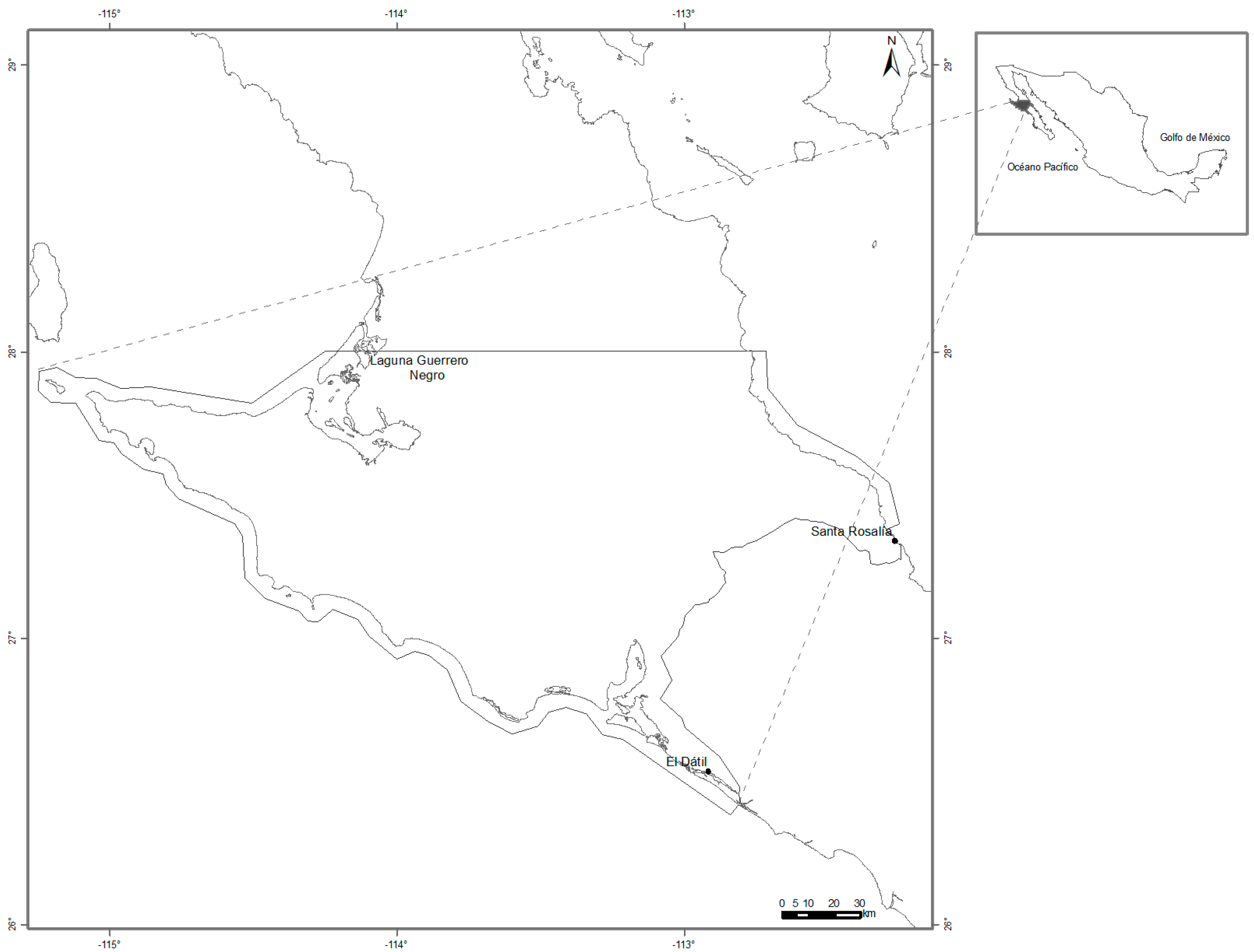
2.1. Study Area

The geographical boundaries of the Vizcaino Reserve are: from the west beginning at the 28th parallel extending from the Laguna Guerrero Negro to the estuary El Datil, and on the east extending from the 28th parallel to Santa Rosalia, and from here to the southeast through the transpeninsular highway, through the Laguna San Ignacio and Barra of San Juan (Figure 1).
The Vizcaino Reserve is one of the largest in Latin America with about 2.55 × 10⁶ ha. It is classified as an arid region, with a dry climate and low annual rainfall [22]. Due to weather patterns and geological conditions, water use by the local population involves pumping from subterranean aquifers.

2.2. Specification of Water Demand Dynamics

Relationships in a model whose character is dynamic by nature can be studied by incorporating the lagged dependent variable among the regressors, known as an autoregressive model. The equation has a bilogarithmic form,
ln w i t = δ ln w i , t 1 + ln z i t ' β + μ i + v i t
where ln w i t is the natural logarithm of the average community water consumption over the course of time t; ln w i , t 1 is the natural logarithm of consumption lagged by one month; z is a matrix of size (n × m) containing m independent variables (price, income, maximum temperature and total monthly rainfall); β is a vector of size parameters (m × 1); μi constitutes the discrepancies among consumers that correspond to each individual community, which is generally not designed by the researcher and is taken into account as a fixed effect. The stochastic component v i t represents the distance between the estimated consumption and consumption frequently observed, and is not inferred by the researcher.
Studies by Nauges and Thomas [23], García [24], and Chang and House-Peters [25] indicate that the use of dynamic models that include a lagged dependent variable generate greater precision in the estimation of parameters, leading to improved predictions surrounding water consumption. Furthermore, it is assumed that demand responds instantaneously to changes in prices, which is the most common means to econometrically evaluate the relationship between demand and consumption. The reason that the dependent variable is lagged is because current consumption is strongly associated with past consumption habits, given that users do not typically change consumption patters for psychological, technological, or institutional reasons. Current consumption estimates therefore depend on data surrounding usage in the previous month, including by household fixtures and appliances such as showers, toilets, washing machines, etc. The frequency of use of such equipment changes gradually over the short-term but may be substantially impacted by replacements or upgrades in the long-term. However, consumers frequently resist upgrading household appliances that consume less water due to the high costs associated with replacements.
Such factors lead to slow reactions by users to changes in prices, as well as gradual adjustments to their consumption. As such, larger displacements are expected to occur in the demand curve in the long-term. Accordingly, it is desirable to formulate a methodology utilizing a partial adjustment model because water is a basic necessity. Therefore, existing inertias in consumption are highly relevant, and these inertias are taken into account by incorporating the lagged dependent variable among the regressors. Furthermore, the average price methodology was selected because users lack information surrounding the pricing structure block, in addition to the marginal price. In the Vizcaino Reserve, consumers receive invoices almost immediately after water is consumed, and payment must be made quickly due to the short time limits imposed by the municipal system. For these reasons, in the economic specification the price was not lagged by one month, based on the recommendations of other studies for situations in which the water bill is delivered to the home between one and two months after consumption has occurred [11,24,26].
Additionally, few previous studies consider inertia in consumption resulting from consumer habits, or from the fact that individuals tend not to respond instantaneously to variations in rates. Thus, current consumption has been assumed to adjust quickly (i.e., during the same period) to the desired level. Such an approach may not be realistic, as illustrated in arguments explained in the partial adjustment model. To not consider real consumption patterns could generate partial and inconsistent estimates. Additionally, the methodology employed by Shin [21] is used in the present study to test their hypothesis, which argues that consumers do not adjust consumption to variations in real prices, but rather to changes in perceived prices. There are several reasons for which it would be too costly for the consumer to determine the actual rate paid for water consumption: (1) It is difficult for consumers to know the difference between the average and the marginal price and the impacts thereof on consumption, given that consumers are typically unaware of the pricing structure block; (2) Even if the consumer was aware of the pricing structure block, it would be difficult to respond immediately to changes in prices and he would only adjust consumption after receiving an invoice for the current billing period; (3) It is very unlikely that the consumer would differentiate water prices from other charges on the invoice, such as sewer service.
In summary, the methodological approach of Shin [21] assumes that consumers consider the marginal costs and marginal benefits in calculating a marginal price without solid foundations, thereby reacting to variations in perceived prices and not to any estimated amount that would reflect actual prices. Depending on how the consumer weighs relevant factors, three responses are possible: (1) If the marginal benefit is less than the marginal cost, the consumer will not respond to the marginal price and will instead determine consumption based on other price information; (2) If the marginal expected benefit is greater than the marginal cost, the consumer will likely determine the real marginal price and the perceived price will equal the marginal price; (3) If the price structure equals the marginal cost, the consumer will stop searching for information and the perceived price will oscillate between the marginal price and the average price.
According to Shin [21] the perceived price is formulated as follows,
P * = M P ( A P / M P ) k
where MP is the marginal price, AP is the average price, and k is a parameter representing price perception. The ratio between AP and MP captures the effect of the difference variable on price perception. It is expected that the parameter k will not be negative. The possible results of k are: (1) When k = 0, the consumer reacts to changes in MP; (2) When k = 1, the consumer reacts to AP; (3) Assuming a structure of prices with increasing blocks (i.e., the rate is progressive), when P * varies between AP and MP, we get the result 0 < k < 1. When k > 1, P * < AP < MP and when k < 0, P * > A P > M P .
The econometric specification is expressed as follows,
ln w i t = β 0 + α ln P M P i t + β ln z i t ' + μ i + v i t = β 0 + α [ ( 1 k ) ln M P + k ln A P ] + β ln z i t ' + μ i + v i t   = β 0   + β 1 ln M P + β 2 ln A P / M P + β ln z i t ' + μ i +   v i t
where β 1 = α ( 1 k ) , β 2 = α k , being k = β2/β1. z is a matrix of size (n × m) containing m independent variables (income, maximum temperature, and total monthly precipitation), β is a vector of size parameters (m × 1). Recent studies by Ito [27] on electric consumption and Wichman [28] on water consumption employed quasi-experimental methods, and their results have demonstrated that behavior is best explained by average price.

2.3. Method of Estimating Water Demand Dynamics

The dynamic panel with fixed effects is the econometric strategy used to estimate the function of water demand, which includes past consumption as a control variable,
y i t = δ y i , t 1 + x i t ' β + μ i t ,     i = 1 , , N ;     t = 1 , , T
with u i t = μ i + v i t , following the approach of Baltagi [29] μ i is fixed and constant for each individual such that v i t ~ IID ( 0 , σ v 2 ) . (I.I.D. means that errors are independent and identically distributed.)
The model also assumes that the explanatory variables are uncorrelated with random error, but may be correlated with individual effects. However, the presence of the lagged dependent variable in the model causes problems of endogeneity because of correlation with the error term [29]. As an alternative solution, Kiviet [30] suggested the use of a Least Squares Dummy Variable (LSDV) as an estimator suitable for finite samples. The correction of bias within the transformation estimator is known as the method of Least Squares Dummy Variable Corrected (LSDVC).
In their Monte Carlo simulations, Judson and Owen [31] demonstrated evidence that when the period is 30, the bias of the fixed effects estimator is considerable. These authors recommend using the LSDVC estimator when the lapse is ≤10 and the Anderson and Cheng estimator [32] when the lapse is significant. Other alternatives exist to correct the problem of endogeneity, such as Instrumental Variables estimators (IV) and the Generalized Method of Moments (GMM). However, these are designed for N with a fixed T, that is, they demonstrate consistency for a large number of cross-sectional units ( N ) , even where the length of the time series is short. Meanwhile, the Arellano and Bond [33] estimator has a significant downward bias in small samples. This is because one of the disadvantages inherent in IV estimators such as Anderson–Hsiao (AH) and Generalised Method of Moments (GMM) estimators such as Arellano–Bond (AB) and Blundell-Bond (BB), is that their asymptotic properties depend on having a large N, which is characteristic of micro panel data.
Recently, Bruno [34] developed a method for utilizing the LSDVC estimator for unbalanced panels. In this method, bias is corrected through a consistent estimator such as AH, AB and BB, where the three alternatives used to initialize the bias correction are asymptotically equivalent. In our case T is relatively large, that is instances of T and N are either few or N is fixed. Cermeño [35], through an empirical study, demonstrated that LSDV estimator bias is lower compared to the estimates that consider T to be small.

2.4. Description of the Database

The present study considered data from the 2010 to 2014 period to inform the econometric model, including information from seven communities: San Ignacio, Bahia Tortugas, Bahia Asuncion, Villa Alberto Alvarado, Guerrero Negro, Mulege, and Santa Rosalia. The description of each is provided in Table 1.
Table 2 shows the descriptive statistics used in the econometric specifications.

3. Results and Discussion

The first step, prior to conducting the econometric analysis of the demand functions, was the analysis of each one of the series represented in the variables. For this analysis, unit root tests were performed on the panel data environment, proposed by: (1) Breitung [36]; (2) Levin et al. [37]; (3) Harris and Tzavalis [38]; (4) Im et al. [39], known as IPS (Im, Pesaran and Shin); and (5) Fisher-type tests [40] known as the Dickey-Fuller (ADF) and Phillips-Perron (PP). The results in Table 3 demonstrate that it was not necessary to apply cointegration vectors, providing support for a methodology involving stationary methods, given that the null hypothesis, which would assume nonstationarity at common levels of significance, is rejected.
Starting with the dynamic panel, the regression results presented in Table 4 show the variation of the demand for residential water attributed to the independent variables considered in the analysis. A significance level of 1%, with a value between 0 < w i , t 1 < 1 , resulted from the analysis of average lagged consumption. The speed of adjustment was obtained by subtracting 1 from 0.62 (its coefficient), the difference being 0.38. The interpretation of this result is that that the gap of 38% separating actual and desired demand for water is closed within a period of one month. With respect to the findings surrounding price elasticity of demand, the expected results were obtained and demand was found to be inelastic, consistent with the general economic theory that postulates an inverse relationship between quantity demanded and price. This result indicates that for user response to the percentage change in price, the percentage change in quantity demanded is less than the percentage change in price.
The short-term elasticity for estimating water demand for domestic use is approximately −0.27 and long-term elasticity is −0.71. The value of the first number is lower than that of the second, suggesting that consumers react primarily to continued increases in rates and not to variations of one month in duration. The permanence of higher prices enables individuals to adapt after one month, thereby adjusting their consumption patterns. The explanation of this result is based on the observation that consumption habits of domestic users tend to remain stable, caused in part by typically minimal variations in water prices. Furthermore, psychological and technological factors may result in gradual rather than immediate adaptation to increases in water rates [23,24]. Schleich and Hillenbrand [41] suggest that the results of the elasticities found in more recent studies could demonstrate a downward trend, possibly because the rates represent a small proportion of household income.
One method for verifying that the estimates of panel data with a lagged dependent variable do not contain inconsistencies and demonstrate that the specification is correct is to compare the estimate of this function with the estimate of a static form such as Equation (4), that is, to identify an alternative assumption in accordance with the suggestion of Angrist and Pischke [42]. The results of the static equation (model 3) of the coefficient MP and AP/MP are similar to those from model 2 from Table 3, and as such the findings are robust.
An important aspect of the analysis is to highlight that endogeneity may originate because the price is considered as an exogenous variable related to water consumption, and if not treated with appropriate econometric techniques it will lead to partial and inefficient estimators. However, we used a database compiled by a representative community, and Shin [43] argues that the endogeneity problem is not very serious in equations that use aggregated information as the original source, compared with equations that use microdata for the synchronization effect created by the existence of a correlation between price and the error term.
Additionally, a test of the error term from Hausman [44] was calculated to check the problem of endogeneity. This was done in order to compare two estimators, one determined to be consistent under the null hypothesis and another an estimator for the instrumental variables (IV). If the null hypothesis is not rejected, the estimator that is considered to be consistent will produce parameter estimates that are unbiased and efficient, and if the null hypothesis is rejected it will produce biased and inefficient estimates. The Hausman statistic was 1.09, indicating that at the 10% significance level the null hypothesis is not rejected, suggesting that the difference in the coefficients is not systematic, and as such there is no evidence for the problem of endogeneity. Of additional relevance is the fact that the water rate is fixed by the operating organism, and does not change based on demand.
Meanwhile, income elasticity of demand demonstrated the positive sign expected according to extant economic theory, with a coefficient of 0.10. This result indicated that for every 1% increase in the income of residential water users, changes in water consumption experienced a corresponding increase of 0.10%. In other words, change manifested as an increase in consumption patterns rather than a change in consumption itself, suggesting that water is a normal good.
With respect to the environmental variables analyzed, maximum temperature was not found to be significant. A negative correlation was found between total monthly rainfall and consumption. This result is logical, because when heavier or more frequent rains fall, water users use less stored water, for example to irrigate, thereby reducing overall consumption. This variable cannot be interpreted as involving directly proportional change, and should therefore be transformed exponentially. When converting the maximum temperature variable, the resulting calculation is 0.9998, indicating that for each additional mm of precipitation, demand is reduced by 0.02%, which is very low. This low coefficient indicates that variations in precipitation have little impact on users’ consumption decisions.
It is important to highlight the similarity between these results and the coefficients obtained through the econometric analysis, which sought to test the hypothesis proposed by Shin [13], in which it is postulated that consumers respond to perceived price. Here, the price perception parameter was 1.08 and the null hypothesis of k = 0 with t = 4.8567 was rejected with 4.8567 at a significance level of 1%; meanwhile, the null hypothesis of k = 1 was not rejected with 0.3730, corroborating the findings suggesting that consumers react to the average perceived price when making usage decisions. Effectively, users believe that the price paid is lower than the actual rate.
According to Shin [21], consumer decisions are based on a perceived price that they believe to be below that specified in institutional rates. However, our results suggest a marginal price lower than the perceived price, indicating that incentives for rational consumption in the short-term are low, which is worrisome given that the study took place in an arid region. For environmental policies and political decision makers, this situation is not ideal because it appears that the rate structure is not achieving at least one of the objectives for which it was designed, that is, promoting water conservation. As such, the rate structure is operating in an environment in which clients do not know with certainty the marginal price that they pay.
Nevertheless, in the long-term the results indicate that permanent increases in prices could improve conservation even if not of the same magnitude as that corresponding to a situation in which users are conscious of the marginal price. Furthermore, the present study could be considered alongside the work of Almendarez-Hernández et al. [45] in which a contingent valuation study was conducted in order to understand the willingness of homes located in the El Vizcaino Biosphere Reserve to pay for improvements of resource availability in the future. Homes would be required to implement conservation practices but supply would be of sufficient quantity and quality. The results obtained signaled a rate increase of 14%.
In the present study, short-term elasticity was −0.26 while elasticity in the long-term was −0.67. These findings are very similar to those reported in recent studies estimating water demand using alternative average price. In a study conducted in France, Nauges and Thomas [23] estimated a dynamic demand function with annual panel data using a non-lineal GMM and a GMM based on Blundell and Bond, with a double-difference estimator. The results obtained included a short-term elasticity of −0.26 and a long-term elasticity of −0.40. Musolesi and Nosvelli [46], with annual panel data from Italy and also using the GMM system, obtained a short-term elasticity of −0.24 and a long-term elasticity of −0.47. Similarly, in Germany, Schleich and Hillenbrand [41] estimated a static model under the Ordinary Least Squares (OLS) method and found an elasticity of −0.242. Fullerton et al. [47] in the region of Halifax in Canada calculated an elasticity of −0.31 using cross-sectional data and an OLS estimator. Finally, with information from Tunisia organized as trimestral, non-seasonal panel data, Younes [48] used a Full Modified OLS method (FMOLS) in which blocks of low and high consumption were segmented, and through which elasticities between −0.08 and −0.46 were found.
Researchers who have employed the price perception methodology introduced by Shin [21] include Nieswiadomy and Molina [49] in Texas, United States of America, with information arranged in monthly panel data and using the IV estimator. This study examined usage in increasing and decreasing blocks, and found elasticities between −0.11 and −0.30. Meanwhile, in the community of Windhoek in Namibia, Kavezeri-Karuaihe et al. [50] used a static model with a full information maximum likelihood (FIML) focus, and obtained elasticities between −0.25 and −0.60. Binet et al. [51], using cross-sectional data from France, estimated an elasticity of −0.31 through an optimal GMM model. In North Carolina, USA, Wichman [28] used a Difference-in-Difference-in-Difference (DDD) model for information ordered in monthly panel data and calculated elasticities between −0.43 and −1.14 and a regression discontinuity framework of −0.31. Similarly, Wichman et al. [52] used panel data in which price and non-price policies were evaluated for periods of drought, and found elasticities between −0.15 and −1.08.
Finally, the results found in the present study are within the range of findings reported in studies that have econometrically evaluated demand functions for residential use in Mexico with a Nordin specification and an average price, such as those discussed in Jaramillo-Mosqueira [53]. This latter study used intra-annual information structured in panel data, employing Discrete-Continuous Choice models and an IV estimator, and calculated elasticities between −0.22 and −0.58. Garcia-Salazar and Mora-Flores [54], also using panel data, found elasticities between −0.18 and −0.20. Salazar and Pineda [55] used IV and Generalized Least Squares (GLS) methods for panel data, and obtained elasticities of −0.33. Avilés-Polanco et al. [56], with monthly time series data, used an IV estimator and found a short-term elasticity of −0.51 and a long-term elasticity of −0.90.

4. Conclusions

The present study presents relevant, quantitative information that could be considered by policy makers for improving their decision-making surrounding water management policies. The results could provide guidance to individuals and institutions responsible for water management practices, empowering them with information with which to evaluate or redesign water rates for residential use. This could be especially useful in contexts in which consumers have imperfect information and it would be too expensive for water managers to invest the requisite time and resources in consumer education.
Furthermore, the findings of the present study surrounding elasticities in water price increases and in relation to inelastic price could lead to the generation of increased revenue, which in turn could be used to improve supply planning. Results could also be considered alongside of those found in other studies applying contingent valuation methods to understand the implementation of conservation programs for aquifer restoration. As such, long-term policies could be designed to provide services to populations without access to potable water and responsible resource use [45,57,58]. For instance, previous studies have examined the willingness of households that are alternately connected or not connected to the drinking water network to pay for improvements to the system in order to ensure resource sustainability in the future, and have found that connected households are more willing to pay.
The introduction of a discriminatory pricing policy that considers seasonality as a factor (i.e., winter and summer) would likely not be as effective for conservation purposes as alternative pricing policies, given its low coefficient. On the other hand, income elasticity of demand was small for this variable, and fell within the range of income elasticity frequently reported in the literature. Estimates suggest that implementing management strategies including instruments such as price are of fundamental importance. Such strategies should be understood as a basis for the evaluation of the functions for which these policies have been structured, and specifically for the development of rates that would satisfy policy objectives. An adequate design of the pricing system for residential water use can complement other social, legal, and environmental policies designed to improve water management in protected natural areas.

Acknowledgments

We would like to thank the National Council of Science and Technology of Mexico (CONACYT) for the financial support that this agency provided for this research (Grants numbers 251460, 269540 of Redes Temáticas and 251919 of Ciencia Básica), as well as the Northwest Biological Research Center of Mexico (CIBNOR), the Biosphere Reserve of Vizcaino, the Municipality of Mulege, and for the support provided by MC. Diana Dorantes and David Jefferson in drafting the English version of this manuscript. We thank the time and effort that Sonia Guan and two anonymous reviewers devoted to improve an earlier version of our manuscript.

Author Contributions

Marco Antonio Almendarez-Hernández and Luis Felipe Beltrán Morales developed the idea. Marco Antonio Almendarez-Hernández, Gerzaín Avilés Polanco, Víctor Hernández Trejo and Alfredo Ortega-Rubio analyzed the data; Marco Antonio Almendarez-Hernández, Gerzaín Avilés Polanco, Víctor Hernández Trejo, Alfredo Ortega-Rubio and Luis Felipe Beltrán Morales wrote the paper.

Conflicts of Interest

The authors declare no conflict of interest.

Abbreviations

The following abbreviations are used in this manuscript:
APAverage price
m3Cubic meters
MPMarginal price
pPrecipitation
tTemperature
wWater consumption average per capita residential use

References

  1. Gleick, P.H. Water in the 21st century. In Water in Crisis; Gleick, P.H., Ed.; Oxford University Press: Oxford, UK, 1993; pp. 105–113. [Google Scholar]
  2. The Food and Agriculture Organization of the United Nations (FAO). El Riego en América Latina y el Caribe en Cifras; FAO: Roma, Italy, 2000; p. 348. [Google Scholar]
  3. The Secretariat of Environment and Natural Resources (SEMARNAT). El Medio Ambiente en México 2005; SEMARNAT: Mexico City, Mexico, 2005. [Google Scholar]
  4. Foro Consultivo Científico y Tecnológico (FCCyT). Diagnóstico del Agua en las Américas; FCCyT: Mexico City, Mexico, 2012. [Google Scholar]
  5. Comisión Nacional del Agua (CNA). Estadísticas del Agua en México; CNA: Metepec, Mexico, 2008. [Google Scholar]
  6. Barkin, D.; Klooster, D. Estrategias de la Gestión del Agua Urbana. En la Gestión del Agua Urbana en México: Retos, Debates y Bienestar; Barkin, D., Ed.; Universidad de Guadalajara: Guadalajara, Mexico, 2006. [Google Scholar]
  7. Beltrán-Morales, L.F.; Borgues-Conterras, J.; Lagunas-Vazquéz, M.; Beltrán-Morales, J.; García-Rodríguez, F. Volúmenes de consume de agua por localidad en la Reserva de La Biosfera del Vizcaíno, B.C.S. México. In Valoración Hidrosocial en la Reserva de la Biosfera del Vizcaíno; Beltrán-Morales, L.F., Chávez López, S., Ortega-Rubio, A., Eds.; CIBNOR: La Paz, Mexico, 2010; pp. 113–128. [Google Scholar]
  8. Almendarez-Hernández, M.A.; Avilés-Polanco, G.; Beltrán-Morales, L.F. Demanda de agua de uso comercial en la Reserva de la Biosfera El Vizcaíno, México: Una estimación con datos de panel. Nova Sci. 2015, 7, 553–576. [Google Scholar] [CrossRef]
  9. Rogers, P.; de Silva, R.; Bhatia, R. Water is an economic good: How to use prices to promote equity, efficiency, and sustainability. Water Policy 2002, 4, 1–17. [Google Scholar] [CrossRef]
  10. PRI Project. Economic Instruments for Water Demand Management in an Integrated Water Resources Management Framework; Policy Research Initiative, The Walter and Duncan Gordon Foundation, Agriculture and Agri-Food Canada, Environment Canada the Canadian Water Network: Edmonton, AB, Canada, 2004. [Google Scholar]
  11. Arbués, F.; Villanúa, I. Potential for pricing policies in water resource management: Estimation of urban residential water demand in Zaragoza, Spain. Urban Stud. 2006, 43, 2421–2442. [Google Scholar] [CrossRef]
  12. Arbués, F.; García-Valiñas, M.; Martínez-Espiñeira, R. Estimation of residential water demand: A state of the art review. J. Socio-Econ. 2003, 32, 81–102. [Google Scholar] [CrossRef]
  13. Worthington, A.C.; Hoffman, M. An empirical survey of residential water demand modelling. J. Econ. Surv. 2008, 22, 842–871. [Google Scholar] [CrossRef]
  14. Billings, R.; Agthe, D. Price elasticities for water: A case of increasing block rates. Land Econ. 1980, 56, 73–84. [Google Scholar] [CrossRef]
  15. Bachrach, M.; Vaughan, W. Household Water Demand Estimation; Working Paper ENP 106; Inter-American Development Bank: Washington, DC, USA, 1994. [Google Scholar]
  16. Charney, A.H.; Woodard, G.C. A test of consumer demand response to water prices: Comment. In Land Economics; University of Wisconsin Press: Madison, WI, USA, 1984; Volume 60, pp. 414–416. [Google Scholar]
  17. Opaluch, J. A test of consumer demand response to water prices: Reply. In Land Economics; University of Wisconsin Press: Madison, WI, USA, 1984; Volume 60, pp. 417–421. [Google Scholar]
  18. Stavins, R.N. Managing Water Demand: Price vs. Non-Price Conservation Programs; A Pioneer Institute White Paper; Pioneer Institute: Boston, MA, USA, 2007. [Google Scholar]
  19. Tracy Mehan, G., III; Kline, I. Pricing as a demand-side management tool: Implications for water policy and governance, Unites States: American Water Works Association. J. Am. Water Works Assoc. 2012, 104, 61–66. [Google Scholar]
  20. Boland, J.; Whittington, D. The Political Economy of Water Tariff Design in Developing Countries: Increasing Block Tariffs versus Uniform Price with Rebate. In The Political Economy of Water Pricing Reforms; Dinar, A., Ed.; Oxford University Press: New York, NY, USA, 2000; pp. 215–235. [Google Scholar]
  21. Shin, J.-S. Perception of Price when Price Information is Costly: Evidence from Residential Electricity Demand. Rev. Econ. Stat. 1985, 67, 591–598. [Google Scholar] [CrossRef]
  22. The Secretariat of Environment and Natural Resources (SEMARNAT); Comisión Nacional del Agua (CNA). Estadísticas del Agua en México; SEMARNAT and CNA: Mexico City, Mexico, 2004. [Google Scholar]
  23. Nauges, C.; Thomas, A. Long-run study of residential water consumption. Environ. Resour. Econ. 2003, 26, 25–43. [Google Scholar] [CrossRef]
  24. García, M. Fijación de precios para el servicio municipal de suministro de agua: Un ejercicio de análisis de bienestar. Hacienda Pública Española/Revista Economía Pública 2005, 172, 119–142. [Google Scholar]
  25. Chang, H.; House-Peters, L. Urban water demand modeling: Review of concepts, methods, and organizing principles. Water Resour. Res. 2011, 47, 1–15. [Google Scholar]
  26. Arbués, F.; Barberán, R. Price impact on urban residential water demand: A dynamic panel data approach. Water Resour. Res. 2004, 40, 1–9. [Google Scholar] [CrossRef]
  27. Ito, K. Do Consumers Respond to Marginal or Average Price? Evidence from Nonlinear Electricity Price. Am. Econ. Rev. 2014, 104, 537–563. [Google Scholar] [CrossRef]
  28. Wichman, C. Perceived price in residential water demand: Evidence from a natural experiment. J. Econ. Behav. Organ. 2014, 107, 308–323. [Google Scholar] [CrossRef]
  29. Baltagi, B. Econometric Analysis of Panel Data, 3rd ed.; John Wiley and Sons: New York, NY, USA, 2005. [Google Scholar]
  30. Kiviet, J. On Bias, Inconsistency, and Efficiency of Various Estimators in Dynamic Panel Data Models. J. Econom. 1995, 68, 53–78. [Google Scholar] [CrossRef]
  31. Judson, R.; Owen, A. Estimating Dynamic Panel Data Models: A Practical Guide for Macroeconomists. Econ. Lett. 1999, 65, 9–15. [Google Scholar] [CrossRef]
  32. Anderson, T.; Cheng, H. Estimation of Dynamic Models with Error Components. J. Am. Stat. Assoc. 1981, 76, 598–606. [Google Scholar] [CrossRef]
  33. Arellano, M.; Bond, S. Some tests of Specification for Panel Data: Monte Carlo Evidence and Application to Employment Equations. Rev. Econ. Stud. 1991, 58, 277–297. [Google Scholar] [CrossRef]
  34. Bruno, G. Approximating the bias of the LSDV estimator for dynamic unbalanced panel data models. Econ. Lett. 2005, 87, 361–366. [Google Scholar] [CrossRef]
  35. Cermeño, R. Median-Unbiased Estimation in Fixed-Effects Dynamic Panels. Ann. D’Econ. Stat. 1999, 55, 351–368. [Google Scholar] [CrossRef]
  36. Breitung, J. The Local Power of Some Unit Root Tests for Panel Data. In Advances in Econometrics; Baltagi, B., Ed.; Elsevier: New York, NY, USA, 2000; Volume 15. [Google Scholar]
  37. Levin, A.; Lin, C.-F.; Chu, C.-S.J. Unit root tests in panel data: Asymptotic and finite-sample properties. J. Econom. 2002, 108, 1–24. [Google Scholar] [CrossRef]
  38. Harris, R.D.F.; Tzavalis, E. Inference for unit roots in dynamic panels where the time dimension is fixed. J. Econom. 1999, 91, 201–226. [Google Scholar] [CrossRef]
  39. Im, K.; Pesaran, M.; Shin, Y. Testing for unit roots in heterogeneous panels. J. Econom. 2003, 115, 53–74. [Google Scholar] [CrossRef]
  40. Baltagi, B.; Chihwa, K. Nonstationary panels, cointegration in panels and dynamic panels: A survey. In Advances in Econometrics; Baltagi, B., Ed.; Elsevier: New York, NY, USA, 2001; Volume 15. [Google Scholar]
  41. Schleich, J.; Hillenbrand, T. Determinants of residential water demand in Germany. Ecol. Econ. 2008, 68, 1756–1769. [Google Scholar] [CrossRef]
  42. Angrist, J.; Pischke, J.-S. Mostly Harmless Econometrics: An Empiricist’s Companion; Princeton University Press: Princeton, NJ, USA, 2009. [Google Scholar]
  43. Shin, J.-S. Aggregation and the Endogeneity Problem. Int. Econ. J. 1987, 1, 57–65. [Google Scholar] [CrossRef]
  44. Hausman, J. Specification tests in econometrics. Econometrica 1978, 46, 1251–1271. [Google Scholar] [CrossRef]
  45. Almendarez-Hernández, M.A.; Jaramaillo-Mosqueira, L.; Áviles-Polanco, G.; Beltrán-Morales, L.F.; Hernández-Trejo, V.; Ortega-Rubio, A. Economic Valuation of Water in a Natural Protected Area of an Emerging Economy: Recommendations for El Vizcaino Biosphere Reserve, Mexico. Interciencia 2013, 38, 245–252. [Google Scholar]
  46. Musolesi, A.; Nosvelli, M. Dynamics of residential water consumption in a panel of Italian municipalities. Appl. Econ. Lett. 2007, 14, 441–444. [Google Scholar] [CrossRef]
  47. Fullerton, T.M., Jr.; Katherine, C.W.; Wm, D.S.; Adam, G.W. An empirical analysis of Halifax municipal water consumption. Canadian Water Resources Association. Can. Water Resour. J. 2013, 38, 148–158. [Google Scholar] [CrossRef]
  48. Younes, B.Z. A long-run analysis of residential water consumption. Econ. Bull. 2013, 33, 536–544. [Google Scholar]
  49. Nieswiadomy, M.; Molina, D. A note on Price Perception in Water Demand Models. Land Econ. 1991, 67, 352–359. [Google Scholar] [CrossRef]
  50. Kavezeri-Karuaihe, S.; Wandschneider, P.R.; Yoder, J.K. Perceived Water Prices and Estimated Water Demand in the Residential Sector of Windhoek, Namibia; Food and Agriculture Organization of the United Nations: Rome, Italy, 2005. [Google Scholar]
  51. Binet, M.-E.; Carlevaro, F.; Paul, M. Estimation of residential water demand with imprecise price perception. Environ. Resour. Econ. 2014, 59, 561–581. [Google Scholar] [CrossRef] [Green Version]
  52. Wichman, C.; Taylor, L.; von Haefen, R. Conservation policies: Who responds to price and who responds to prescription? J. Environ. Econ. Manag. 2016, 79, 114–134. [Google Scholar] [CrossRef]
  53. Jaramillo-Mosqueira, L. Evaluación econométrica de la demanda de agua de uso residencial en México. Trimestre Económico 2005, 72, 367–390. [Google Scholar]
  54. García-Salazar, J.A.; Mora-Flores, J.S. Tarifas y consumo de agua en el sector residencial de la Comarca Lagunera. Región Sociedad 2008, 20, 119–132. [Google Scholar]
  55. Adams, A.S.; Pablos, N.P. Factores que afectan la demanda de agua para uso doméstico en México. Región Sociedad 2010, 22, 3–16. [Google Scholar]
  56. Avilés-Polanco, G.; Almendarez-Hernández, M.; Hernández-Trejo, V.; Beltrán-Morales, L. Elasticidad-precio de corto y largo plazos de la demanda de agua residencial de una zona árida. Caso de estudio: La Paz, B.C.S., México. Tecnología Ciencias Agua 2015, 4, 85–99. [Google Scholar]
  57. Avilés-Polanco, G.; Huato, L.; Troy-Diéguez, E.; Murillo, B.; García, J.; Beltrán-Morales, L. Valoración económica del servicio hidrológico del acuífero de La Paz, B.C.S.: Una valoración contingente del uso de agua municipal. Frontera Norte 2010, 22, 103–128. [Google Scholar]
  58. Sánchez-Brito, I.; Almendarez-Hernández, M.A.; Morales-Zárate, M.V.; Salinas-Zavala, C.A. Valor de Existencia del Servicio Ecosistémico Hidrológico en la Reserva de la Biosfera Sierra La Laguna, Baja California Sur México. Frontera Norte 2013, 25, 97–129. [Google Scholar]
Figure 1. Area of Biosphere Vizcaino Reserve.
Water 08 00428 g001
Table 1. Description of variables used in the regression analysis.
VariableDescriptionSource
w Symbolizes average water consumption per capita in residential use. The variable is measured in cubic meters (m3).System Operator Agency Water Supply and Sewerage (OOMSAPA).
APAverage price, obtained by dividing the water bill paid by the consumer living in one housing unit and the volume of water consumed. Additionally, the measurement of price was deflated using the National Consumer Price Index (NCPI), base 2010 = 100, where 2010 is the bases year for the estimation, obtained from the Bank of Mexico (BM).System Operator Agency Water Supply and Sewerage (OOMSAPA).
MPMarginal price, representing the amount that the consumer must pay, according to the fee structure for final consumption units associated with the average amount. The price was deflated using the CPI, base 2010 = 100.System Operator Agency Water Supply and Sewerage (OOMSAPA).
IncomeDefined as the average daily wage by state according to the Mexican Social Security Institute (IMSS). In the regression analysis it is used as a proxy for income, representing an indicator of household income. For purposes of inclusion in the dynamic equations, we calculated monthly wage. This variable was deflated with CPI base 2010 = 100 and weighted with the working population.National Commission for Minimum Wage in the State of Baja California Sur.
tMonthly maximum temperature, measured in degrees Celsius (°C).National Water Commission (CONAGUA).
PTotal monthly precipitation, measured in millimetres (mm).National Water Commission (CONAGUA).
Table 2. Descriptive statistics of variables selected for the regression analysis.
VariableMeanStandar DevationMinimunMaximun
Natural Logarithm of Water Consumption3.080.391.273.92
Natural Logarithm of Average Price1.590.371.223.22
Natural Logarithm of Income8.440.048.338.5
Natural Logarithm of Temperature3.480.182.893.78
Natural Logarithm of Precipitation9.525.150218
Natural Logarithm of Marginal Price1.490.191.122.88
Table 3. Results of unit root tests of the dynamic function variables.
TestVariable
Natural Logarithm Water ConsumptionNatural Logarithm Average PriceNatural Logarithm of IncomeNatural Logarithm TemperatureNatural Logarithm Marginal PricePrecipitation
Levin, Lin and Chu t-stat 1No trend−3.5058 *−2.9591 *−4.7032 *−3.3096 *−5.3825 *−14.8757 *
Trend−3.7844 *−3.6753 *−4.5454 *−2.9802 *−7.1843 *−16.4279 *
Breitung t-stat 1No trend−2.016 **0.8364−2.8989 *−3.8967 *−3.8093 *−11.1172 *
Trend−2.9742 *−1.7696 **−1.6902 **−3.1495 *−1.5693−11.1841 *
Harris-Tzavalis 1No trend−12.4917 *−9.9615 *−39.8499 *−14.5436 *−29.5214 *−39.8661 *
Trend−8.4543 *−8.6226 *−30.2714 *−7.3701 *−24.2629 *−24.5517 *
Im, Pesaran and Shin W-stat 2No trend−4.7914 *−5.1862 *−6.9979 *−9.5987 *−7.1840 *−13.172 *
Trend−4.9233 *−3.7272 *−13.1415 *−8.9286 *−9.8964 *−13.7871 *
ADF-Fisher Chi-square 2No trend61.273 *24.9921 **76.8509 *117.714 *87.2638 *170.723 *
Trend55.8855 *36.2216 *158.721*98.8576 *112.370 *161.536 *
PP-Fisher Chi-square 2No trend61.0525 *42.2184 *209.668 *81.1587 *83.0181 *183.702 *
Trend54.2991 *59.9753 *234.038 *57.8068 *105.175 *156.455 *
Notes: * The null hypothesis of unit root is rejected at 1%; ** The null hypothesis of unit root is rejected at 5%; 1 Represents a common unit root process; 2 Represents an individual unit root process.
Table 4. Estimates of the dynamic function.
VariableModel 1Model 2Model 3
Coefficientt-RatioProbabilityCoefficientt-RatioProbabilityCoefficientt-RatioProbability
Constant0.64261.41730.15720.57681.21100.29401.07901.36210.1739
Lagged consumption0.617113.2977 *0.00000.611612.2336 *0.0000---
AP−0.2735−5.9151 *0.0000------
MP---−0.2587−4.3048 *0.0000−0.2830−5.5984 *0.0000
AP/MP---−0.2803−5.6858 *0.0000−0.3123−7.5952 *0.0000
Income0.10471.7747 ***0.07670.11271.8093 ***0.07120.13291.8579 ***0.0639
Temperature0.02591.35920.17480.02451.27850.20180.05571.11240.2666
Precipitation−0.00015−2.5679 **0.0106−0.00015−2.4170 **0.0161−0.00017−2.8669 *0.0043
k---1.08324.8567 *0.0000---
R20.92530.9251-
F Test of fixed effects13.1292 *, 0.000013.0892 *, 0.0000-
DURBIN-WATSON2.14972.1507-
Notes: To compute the ratios t, heterostedasticity robust standard errors were used. * Significant at 1%; ** Significant at 5%; *** Significant at 10%.

