Article

Interannual Variability in Global Mean Sea Level Estimated from the CESM Large and Last Millennium Ensembles

1
National Center for Atmospheric Research, Boulder, CO 80301, USA
2
Department of Atmospheric and Oceanic Sciences, University of Colorado, Boulder, CO 80309-0311, USA
3
Department of Aerospace Engineering Sciences, University of Colorado, Boulder, CO 80309-0311, USA
*
Author to whom correspondence should be addressed.
Water 2016, 8(11), 491; https://doi.org/10.3390/w8110491
Submission received: 24 September 2016 / Revised: 25 October 2016 / Accepted: 26 October 2016 / Published: 31 October 2016
(This article belongs to the Special Issue Sea Level Changes)

Abstract

:
To better understand global mean sea level (GMSL) as an indicator of climate variability and change, contributions to its interannual variation are quantified in the Community Earth System Model (CESM) Large Ensemble and Last Millennium Ensemble. Consistent with expectations, the El Niño/Southern Oscillation (ENSO) is found to exert a strong influence due to variability in rainfall over land (PL) and terrestrial water storage (TWS). Other important contributors include changes in ocean heat content (OHC) and precipitable water (PW). The temporal evolution of individual contributing terms is documented. The magnitude of peak GMSL anomalies associated with ENSO generally are of the order of 0.5 mm·K−1 with significant inter-event variability, with a standard deviation (σ) that is about half as large The results underscore the exceptional rarity of the 2010/2011 La Niña-related GMSL drop and estimate the frequency of such an event to be about only once in every 75 years. In addition to ENSO, major volcanic eruptions are found to be a key driver of interannual variability. Associated GMSL variability contrasts with that of ENSO as TWS and PW anomalies initially offset the drop due to OHC reductions but short-lived relative to them. Responses up to 25 mm are estimated for the largest eruptions of the Last Millennium.

1. Introduction

Global mean sea level (GMSL) is a key indicator of the Earth’s energy and water cycles. It has been precisely and accurately estimated from satellite altimetry for over two decades and reconstructions from tide gauges extend into the early 19th century [1,2], with individual gauge records extending back to the early 18th century. As such, it has considerable potential for providing insight into climate change and variability over both the recent and more distant past. However, interpreting the sea level record is nontrivial as it includes contributions from various reservoirs of water and energy in the atmosphere, ocean, land surface, and cryosphere [3]. Moreover, surface winds and gravitational effects influence its spatial patterns [4,5,6]. Understanding the climatic implications of the sea level record therefore depends crucially on being able to disentangle these diverse and multiple effects.
For the past decade, a detailed understanding of variability in global mean sea level has been made possible by advances in observing systems. These include the ARGO array of in-situ ocean observing sensors, providing ocean temperature data of unprecedented sampling density, accuracy, and stability [7], and the GRACE satellites, which provide surface mass variability estimates [8]. In conjunction with satellite altimetry [9], these data have allowed for the closure of the global ocean height budget on annual timescales to within about 1 mm, mainly through joint consideration of ocean heat content (OHC) and terrestrial water storage (TWS). Key insights from this record have related primarily to the quantitative understanding of specific events, and, specifically, extremes in El Niño and La Niña [10,11,12,13,14,15,16].
However recent observations have also raised several questions. For example, the reported magnitude of variability has been difficult to relate directly to ENSO strength. An increase in GMSL of about 2 mm was reported for one of the strongest El Niño events of the 20th Century (1997/1998, [15]) and attributed to TWS deficits driven by reductions in rainfall over land (PL), an influence that has been identified generally for ENSO [11,17]. In contrast, the 2010/2011 La Niña was associated with a drop estimated to be approximately three times as large (~7 mm) while being strong yet comparable to other La Niña events of the 20th century. What drove this disparity? Is it a consequence of errors in altimeter retrievals, an intrinsic asymmetry between El Niño and La Niña, or is it indicative of broader inter-event variability relating to ENSO generally? If the latter, in what continents and ocean basins does inter-event variability mainly reside and why? What other water reservoirs influence GMSL and how can their contributions be quantified?
In part, these issues have been previously addressed [16] and TWS variability has been shown to be susceptible not only to ENSO, but to other internal modes of variability, their influence on PL, and the hydrologic character of key land regions. In revealing the importance of such effects, recent work has also implicitly highlighted the limitations of quantifying such complex and episodic land-ocean exchanges with brief satellite records due to large inter-event variability. More generally, a major outstanding issue relating to interannual GMSL variability is the influence of volcanic effects, as the GRACE, ARGO, and altimeter records have yet to monitor a major eruption. Observations of PL and OHC anomalies suggest opposing influences during eruptions [18,19] and modeling studies have estimated the associated OHC component [20,21,22,23,24,25,26]. However, what is the full impact of volcanic eruptions on sea level, how can it best be estimated, and what variations have likely occurred in the recent and distant past?
To address these questions, simulations from the CESM Large and Last Millennium Ensembles are evaluated and the dominant contributors to interannual GMSL variability, including OHC and TWS but also extending beyond to include atmospheric precipitable water (PW), are quantified. Spanning thousands of years of simulations, these runs are based on one of the best available coupled climate models [27] and up to date estimates of external forcing. The structure and merits of these runs is discussed in Section 2 while the simulated influence of ENSO on global budgets is assessed in Section 3. The roles of terrestrial contributions to TWS by continent and ocean OHC variability by basin are discussed in Section 4 while volcanic effects are assessed in Section 5. Implications for our understanding of GMSL are summarized and conclusions, including suggested future priorities, are discussed in Section 6.

2. Materials and Methods

To provide a comprehensive accounting of internal variability, simulations are provided from the CESM Large Ensemble (LE) [28] and Last Millennium Ensemble (LME) [29]. The LE provides 40 members of fully coupled simulations extending from 1920 to 2100 using a single model and set of external forcings. The runs are initialized from a single member in 1920, at which time they are perturbed with roundoff error (~10−14 K) differences to their air temperature fields. Within a matter of months, the major modes of atmospheric internal variability diverge, providing a broad sample of coupled climate realizations. The horizontal resolution of the LE is approximately 1° in all model components. The CESM uses the Community Land Model 4 (CLM4) [30,31] and LANL Parallel Ocean Program, version 2 (POP2) [32] for its land and ocean components, respectively. The CLM4 is designed to represent the physical, chemical, and biological processes by which terrestrial ecosystems interact with climate across a variety of spatial and temporal scales and reproduces with exceptional fidelity the observed variability in GRACE-era TWS [26,31,33]. Over ice sheets, the CLM uses a mass balance scheme that neglects ice sheet dynamics. To avoid snow build-up, CLM employs snow capping at 1 m snow water equivalent beyond which snow gets sent directly to runoff as an “ice stream” to approximate calving and maintain ice sheet balance. Its ability to capture low frequency cryospheric mass variability is therefore limited, however, for the timescales of interest here, such effects are small [34]. The POP2 is a primitive equation model that resolves 60 vertical levels, which vary in depth from 10 m near the surface to 250 m at depth. External forcings are based on the historical and RCP8.5 pathways from CMIP5 scenarios and include variability in greenhouse gases, volcanic aerosols, and other forcing agents.
The LME provides a 10 member set of fully-forced simulations spanning 850 to 2005 using the PMIP3 forcings prior to 1850 and CMIP5 historical forcings thereafter that include variations in land use and land cover, solar intensity, orbital parameters, greenhouse gas concentration, and volcanic and anthropogenic aerosols. Model components are identical to those used for the LE, but the atmosphere is run at 2° horizontal resolution. Here, the CESM-LME will be used to provide a longer-term perspective for understanding the influence of major volcanic events since 850 on GMSL.
Together, the LE and LME provide a unique opportunity to explore the processes governing GMSL’s interannual variability. One of the key improvements in CESM over earlier model is the simulation of variability associated with the El Niño–Southern Oscillation (ENSO) including a lengthened and more realistic periodicity, and a longer duration of La Niña compared to El Niño [35]. Closure of the energy and water budgets is a major advance of the CESM, building on the improvements achieved in Community Climate System Model Version 4 particularly as related to TWS simulation [31,33], making the CESM ideal for exploring sea level relevant processes. As the POP2 is a fixed volume ocean, however, GMSL is not explicitly simulated. To estimate this influence, GMSL contributions from OHC, TWS (which includes contributions from snow and ice but not ice sheets), and atmospheric water (PW) are estimated as in:
GMSL’ = TMQ’ × AA/AO + TWS’ × AL/AO + OHC’ × C
where the areas of the globe (AA, 0.51 × 10¹⁵ m2), land (AL, 0.14 × 10¹⁵ m2), and ocean (AO, 0.37 × 10¹⁵ m2) are used and OHC is converted to sea level rise using the conversion of 3 × 10²² J as equivalent to 5 mm of thermosteric sea level rise (C = 5 mm/3 × 1022 J, [36]). TWS is computed from individual CLM terms such that:
TWS= ∫ (SOILLIQ + SOILICE) + WA + H2OSNO + H2OCAN + VOLR
where soil liquid (SOILLIQ) and ice (SOILICE) are integrated through the depth of the soil column and added to water storage in aquifers (WA), snow cover (H2OSNO), the canopy (H2OCAN), and rivers (VOLR).
ENSO events are defined in a manner consistent with the Objective Niño Index based on the method employed by the NOAA/Climate Prediction Center (3-month running mean of SST anomalies in the Niño 3.4 region, 5 N–5 S, 120–170 W) where the 30-year running mean is first removed. Anomaly thresholds of 2 K for El Niño events and 1.7 K for La Niña events are used in order to provide a comparable sampling of about 500 events of each type (~1 per decade) while accounting for asymmetry in the strengths of warm and cold events. These thresholds are also consistent with some of the stronger ENSO events observed in nature, such as the warm events of 1972/1973, 1982/1983, and 1997/1998 and cold events of 1975/1976, 1988/1989, and 1999/2000.

Model Evaluation

Despite the successes of the CESM [35], it is important to evaluate the model for its suitability for the budgets evaluated, depending critically on model being able to reproduce ENSO, its main rainfall teleconnections, and variability in the planetary energy budget. Figure 1 shows ONI regressed annual (July–June) rainfall amounts in the LE from where the choice of months in the average is intended to maximize coherence with ENSO. Regions are also indicated where the LE distribution of members lies above (hatched) and below (stippled) regressions based on observations from the Global Precipitation Climatology Center Version 6 [37] and HADISST [38] datasets. The broad regression pattern in the simulations generally resembles that in observations, exhibiting strong negative values in northern South America, Australia, and Southeast Asia. The main region of disagreement is in equatorial Africa, where observations show insignificant relationships while the model depicts strong positive regressions. Discrepancies in magnitude also exist regionally, such as weaker observed relationships in Australia, southwest North America, and Eurasia, and stronger observed relationships in northern and southern South America. Despite these disagreements, continental scale relationships agree generally with GPCC, particularly in South America and Australia where TWS variations are particularly important (|m| > 0.75 mm/day/K) [14,16] with weaker continent wide regressions reported elsewhere.
The fidelity of the CESM simulation of ENSO is also a key concern and the associated Niño3.4 power spectrum is shown in Figure 2 and compared to HADISST observations. While the overall form of the simulated power spectrum agrees well with observations and represents a major advance from earlier model versions [35], the power at periodicities near four years is too strong (although also highly variable across 100-year ensemble members). To account for this, large-scale contributions to GMSL are normalized by Niño3.4 SST, as they are found to relate approximately linearly to ENSO strength.
Variability in the planetary imbalance as estimated by the top-of-atmosphere imbalance (RT) relates strongly to OHC and is perhaps the strongest observational constraint on OHC interannual variations given the major challenges involved in their direct estimation [39]. To evaluate CESM variability, the estimate of the planetary imbalance (A14, [40]) is therefore used and compared with the distribution of members from the LE in Figure 2. The major forced change is that associated with the 1991 eruption of Mt. Pinatubo, which drove the annual mean planetary imbalance to be between −1 to −2 W·m−2, a value that agrees closely (within 0.2 W·m−2) with observed estimates. The time series exhibit a similarly strong agreement in the onset and decay of the anomaly. At other times in the record, variability is driven mainly by ENSO and both the mean imbalance and its temporal variability agrees well with simulated behavior, with excursions beyond the σ range occurring infrequently and beyond the 2 × σ range occurring only during the exceptional 1997/1998 El Niño.

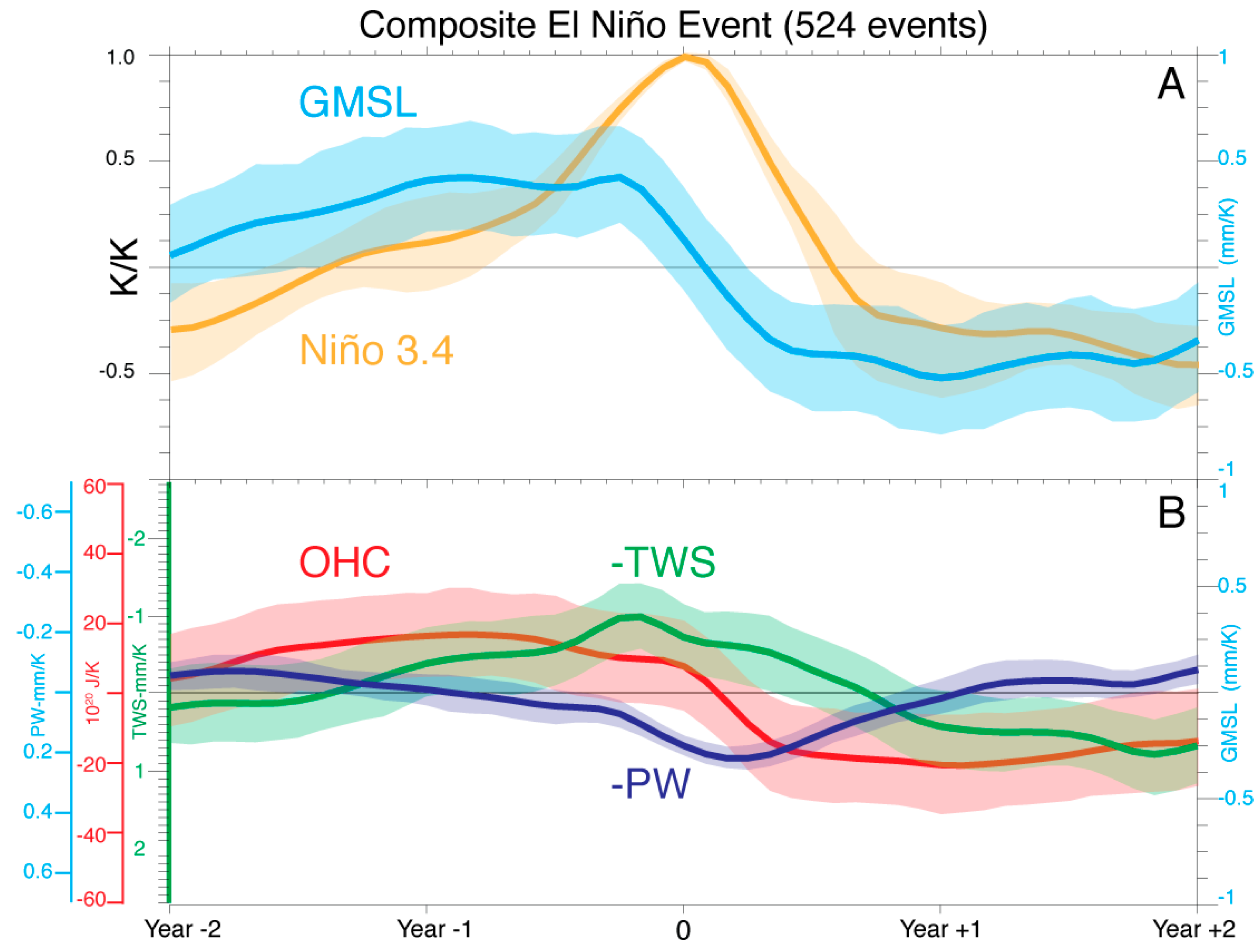
3. GMSL Variability during ENSO

Variability during ENSO is characterized generally by asymmetric transitions from El Niño to La Niña. The onset of El Niño begins in the year prior to its peak and is followed generally by the transition to unusually cool conditions in the year thereafter, often associated with a transition to La Niña (Figure 3). During El Niño onset, OHC anomalies are positive generally and PL and TWS anomalies are negative as rainfall migrates away from low latitude land regions generally (e.g., Figure 1) and toward ocean. Together, these influences contribute to an increase in GMSL. In the months following the peak of El Niño, OHC decreases rapidly as energy is released to the atmosphere [39,41] leading to increases in PW, which accompany a warming of the troposphere to maintain approximately constant relative humidity. SST cools and negative PL anomalies dissipate, leading to increases in TWS. Together these factors lead to a rapid reduction in GMSL following the peak of El Niño events. The magnitude of GMSL anomalies in both the onset (GMSL’ > 0) and decay phases (GMSL’ < 0) is roughly 0.5 mm·K−1, though considerable inter-event variability exists (σ of about 0.25 mm·K−1).
The onset of La Niña events (Figure 4) is characterized by the preceding influence of negative OHC anomalies associated with El Niño. As La Niña ensues, PL and associated TWS anomalies increase, contributing to negative GMSL anomalies that strengthen as La Niña peaks. OHC increases following the peak of La Niña, as the atmosphere cools and PW anomalies become negative, contributing to a gradual increase in GMSL that is offset somewhat by persistent positive TWS anomalies. A year after the peak in La Niña, positive TWS anomalies are partially offset by negative PW anomalies and GMSL is near normal as a result. As for El Niño events, considerable inter-event variability exists with a σ range of approximately 0.5 mm·K−1. Given this canonical behavior, events such as the 2010–2011 sea level drop of approximately 7 mm are exceedingly rare in the LE, with drops of comparable magnitude occurring once in about every 75 years.

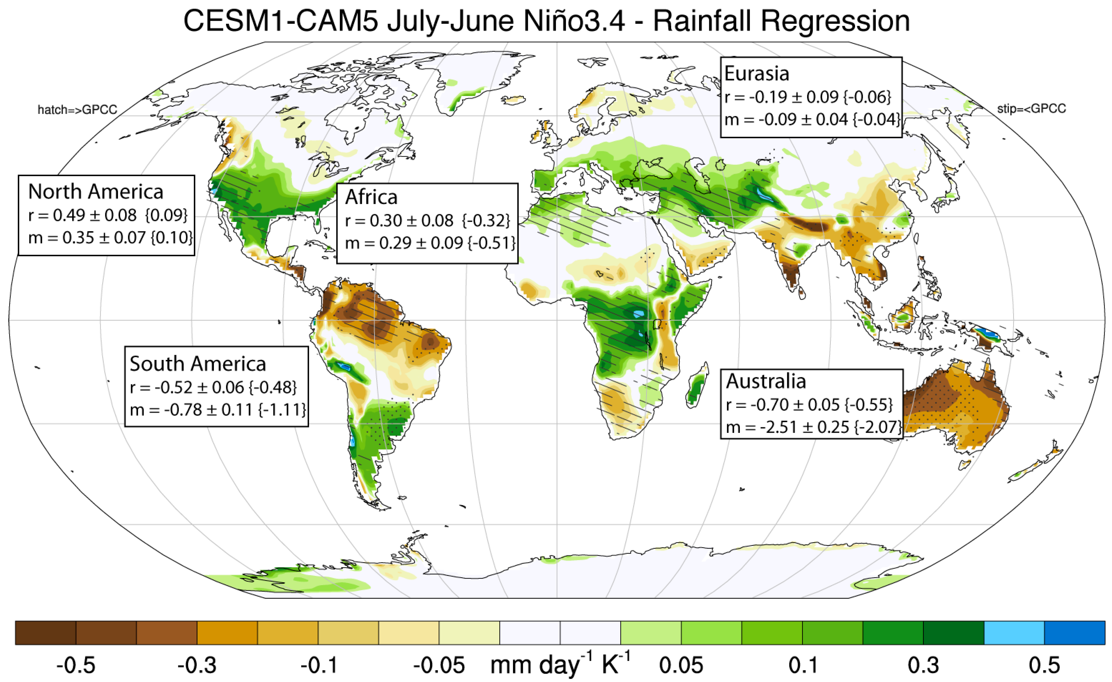
4. Regional Sources of GMSL Variability

The continents and ocean basins that contribute to TWS and OHC anomalies during El Niño (Figure 5) reveal the specific regional character of contributions to GMSL variability. TWS variability is dominated by the combined and contrasting influences of Australia and South America (SA). At the peak of El Niño, TWS deficits in SA are typically the single largest contributor to the global-land anomaly, however, its contributions vary rapidly relative to those from Australia, where they persist for more than a year following most events and exceed those from SA despite the continent being less than half as large. The contrast is likely associated with the contrasting hydrology of the two continents [16]. The onset of El Niño events is characterized by significant positive anomalies in Pacific OHC, roughly a year prior to El Niño’s peak. Anomalies in other ocean basins at this time are small generally. During El Niño events, rapid OHC decreases are also unique to the Pacific and dominate variability in global OHC. The Indian and Atlantic Ocean basins compensate for variability in the Pacific with a net increase in OHC in a manner similar to that observed [41].
Regional variability associated with La Niña (Figure 6) is influenced initially by preceding El Niño conditions, with negative TWS anomalies in Australia and SA and negative OHC anomalies in the Pacific Ocean. During La Niña, these anomalies dissipate and are followed by strong positive TWS anomalies, both in SA and in Australia (where they again are persistent), and a recovery of OHC in the Pacific Ocean.

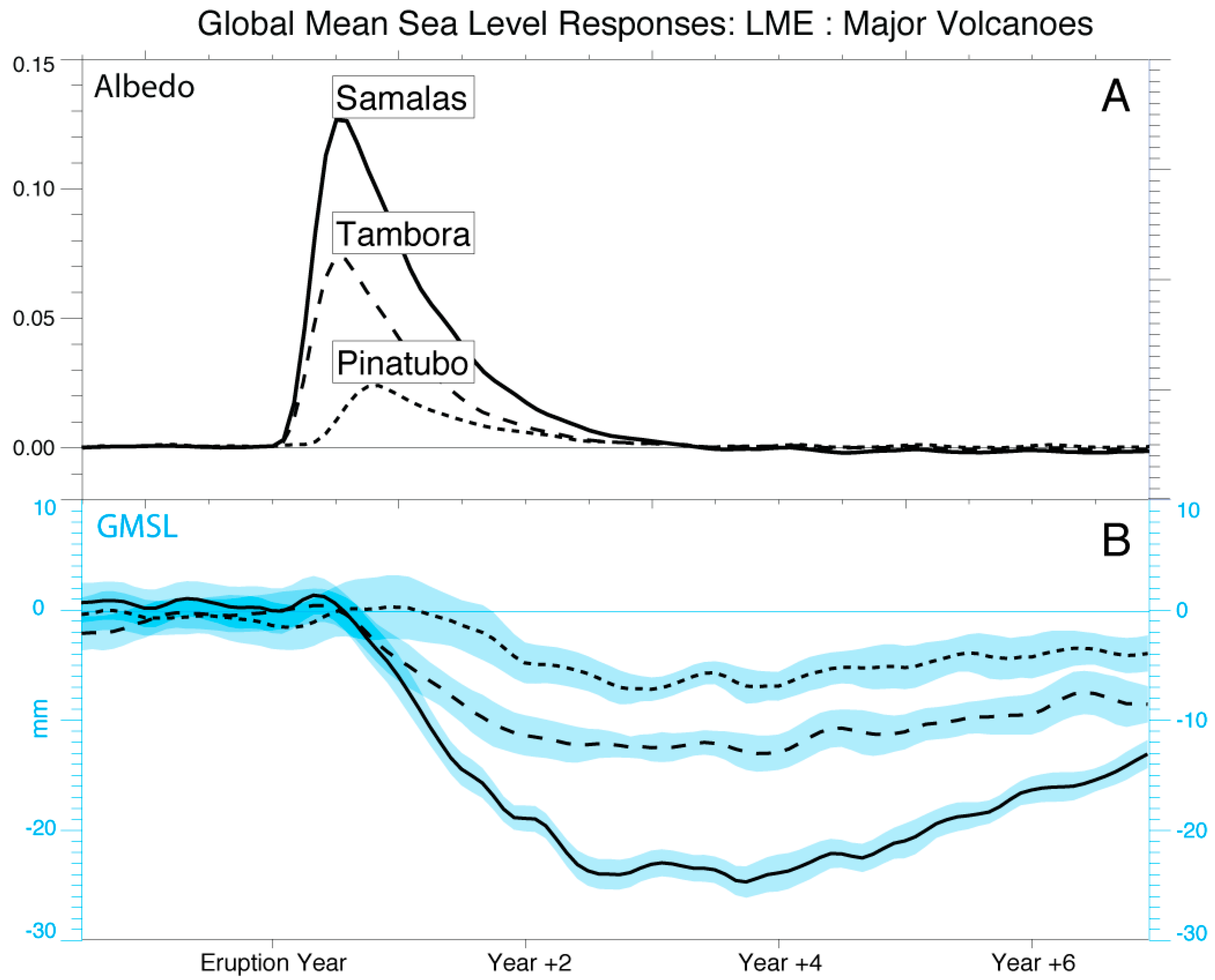
5. GMSL Variability Following Volcanic Eruptions

Beyond ENSO, major volcanic eruptions are also key drivers of interannual GMSL variability simulated by the LE and LME. As an example, the largest volcanic eruption of the past several centuries is the eruption of Mt. Tambora [42] and its modeled GMSL influence is summarized in Figure 7. Variations in OHC are generally much larger during major volcanic eruptions than during ENSO [26] and their GMSL influence is mainly moderated by changes in PW and TWS, rather than being accentuated by them. Following the Tambora eruption, a reduction in GMSL is estimated at about 12 mm by the LME, mainly due to the decrease in OHC associated with the increased planetary albedo arising from a spike in stratospheric aerosols. Immediately following the eruption, a decrease in TWS is simulated due to an overall weakening of the hydrologic cycle, as less sunlight becomes available at the surface to energetically balance evaporation, and due to a disproportionate weakening of rainfall over land, where the surface also cools disproportionately. As the surface and atmosphere cool in response to the eruption, atmospheric water storage decreases. Changes in both PW and TWS thus moderate the initial reduction in GMSL somewhat, though at the time of peak OHC reduction, these anomalies have decreased such that the maximum OHC anomalies goes approximately unchecked. Also relevant for the GMSL budget is the fact that there is a heightened probability of El Niño in two winters after the eruption followed by La Niña [43] due to volcanic forcing and this influences subsequent GMSL variability as described above superimposed on the GMSL variability that would be expected from the recovery in OHC alone.
To provide a broader context for the GMSL drop during the 1815 Tambora eruption, simulations from the LME full forcing runs are used (Figure 8). The largest recent eruption is the 1991 eruption of Mt. Pinatubo in the Philippines [26] while other more massive eruptions are known to have occurred in the last millennium, such as Indonesia’s Mt. Samalas eruption in 1258 [44]. These eruptions are associated with albedo increases that are about half and twice as large as that of Mt. Tambora, respectively. The LME simulations depict a reduction in GMSL due to Pinatubo’s eruption similar to that of the LE (approximately 6 mm, [26]) while depicting much larger drops and longer recovery timescales for the eruptions of Tambora and Samalas. Peak ensemble mean reductions during these eruptions are estimated at about 12 mm and 25 mm, respectively. The associated timescale of recovery is considerable with an e-folding timescale of GMSL anomalies of approximately a decade for Samalas’ eruption.

6. Discussion and Conclusions

The contributions to interannual variability in GMSL have been quantified using the multi-member ensembles provided by the CESM Large and Last Millennium Ensemble projects. The analysis provides a means for quantifying and understanding variability to a degree that is not currently possible using observations, yet is critical for interpreting associated variability and related issues such as sea level rise acceleration [26,45] in modern data records. The simulation of ENSO and volcanic eruptions in these ensembles agree well with available observations and the transient nature of associated contributions is documented.
At the onset of El Niño, OHC anomalies in the Pacific become positive and TWS decreases due to reductions in rainfall over land, and particularly in SA and Australia, leading to positive GMSL anomalies. At the peak of El Niño, OHC in the Pacific undergoes a dramatic reduction, warming the atmosphere and increasing PW. TWS begins to increase following the peak of El Niño and together with PW increases and rapid decreases in OHC lead to a transition to negative GMSL anomalies as the system tends toward La Niña conditions. As La Niña intensifies, positive rainfall and TWS anomalies over land grow while OHC anomalies remain negative, leading to negative GMSL anomalies. A cooler atmosphere contributes to negative PW anomalies, thus offsetting somewhat reductions in GMSL. As La Niña conditions wane, OHC, PW, and terrestrial rainfall return to climatological values while TWS anomalies persist, particularly in Australia, prolonging the drop in GMSL.
While the simulations provide an unparalleled opportunity to quantify and diagnose GMSL variability, important caveats exist. A main caveat lies in the apparently erroneous teleconnections simulated by CESM in equatorial Africa, where positive rainfall teleconnections are simulated contrary to observations, which show no significant correlations. While data records in this region are known to suffer from poor quality control [46], neighboring SST gradients are also poorly simulated in the model, suggesting an associated rainfall bias. The net effect of the bias would be to increase the net GMSL response to ENSO simulated by the CESM, as local TWS anomalies oppose those in SA and Australia and lessen the associated global-land TWS response. The excess power associated with ENSO in the CESM is also a source of concern. The finding of approximately linear responses to SST and the associated normalization of anomalies helps address this issue, however it would be useful to corroborate these findings in next-generation models that provide an improved depiction of ENSO, terrestrial hydrology, volcanic forcing, and associated energy budget anomalies.
Despite these caveats, a number of key findings are likely to be robust. Chief amongst these is that GMSL fluctuations during ENSO on average are the result of changes in both TWS and OHC, with secondary but non-negligible contributions from PW. In addition, large inter-event variability is evident, suggesting an interaction with other climate modes [16] or stochastic variability. It is therefore unsurprising that the behavior of individual events in the modern altimeter and gravity records spans a broad range. Regional analysis suggests a disproportionate role for TWS in Australia and SA and OHC in the Pacific Ocean in influencing global TWS and OHC budgets, respectively. A unique low frequency influence of Australian hydrology on TWS is also corroborated, both during El Niño and La Niña events. Nonetheless, the frequency of sea level drops in these simulations comparable to that observed from 2010 to 2011 was found to be rare, occurring about once in every 75 years.
Beyond ENSO events, volcanic events are identified as drivers of significant GMSL interannual variability. They are distinct from ENSO in that they have a larger OHC signature and their associated GMSL response is moderated, rather than enhanced, by both TWS and PW anomalies as the land and atmosphere dry and cool. Nonetheless, the GMSL drop during the 1991 eruption of Mt. Pinatubo is estimated at about 6 mm with drops during the major eruptions of Mts. Tambora and Samalas estimated at about 12 mm and 25 mm, respectively.
Extending these results to the modern-day altimeter record has several broader implications. As shown in recent work [26], the influence of Mt. Pinatubo’s 1991 eruption is likely to have masked acceleration in the altimeter record. However, it remains an open question as to how soon acceleration in that record will become evident. At the time of this manuscript, conditions in the Pacific have transitioned from a strong El Niño event in early 2016 to ENSO-neutral conditions. The current analysis suggests that the associated GMSL signature of such a transition should occur rapidly as the positive GMSL anomaly associated with El Niño typically decays within a few months of its SST maximum (Figure 3). Meanwhile, available altimeter products show persistent strong positive GMSL anomalies into mid-2016. A major outstanding question is therefore whether these anomalies have been maintained by an El Niño event that deviates from the CESM’s composite mean behavior or whether they are the early signs of acceleration in the GSML record.

Acknowledgments

John T. Fasullo’s participation in this work is supported by NASA award NNX13AI26G, NSF award NSF-AGS-1243107, and DOE Award ID DE-SC0012711. Robert S. Nerem was supported by NASA Award NNX13AI26G.

Author Contributions

John T. Fasullo conceived and designed the analysis, analyzed the data, contributed software analysis tools, and wrote the original draft of the manuscript. Robert S. Nerem was involved in the discussions in which this work was conceived and contributed to finalizing the submitted version.

Conflicts of Interest

The authors declare no conflict of interest. The founding sponsors had no role in the design of the study; in the collection, analyses, or interpretation of data; in the writing of the manuscript, and in the decision to publish the results.

References

  1. Nerem, R.S.; Haines, B.J.; Hendricks, J.; Minster, J.F.; Mitchum, G.T.; White, W.B. Improved determination of global mean sea level variations using TOPEX/POSEIDON altimeter data. Geophys. Res. Lett. 1997, 24, 1331–1334. [Google Scholar] [CrossRef]
  2. Jevrejeva, S.; Moore, J.C.; Grinsted, A.; Matthews, A.P.; Spada, G. Trends and acceleration in global and regional sea levels since 1807. Glob. Planet. Chang. 2014, 113, 11–22. [Google Scholar] [CrossRef] [Green Version]
  3. Church, J.A.; Cazenave, A.; Gregory, J.M.; Jevrejeva, S.; Levermann, A.; Merrifeld, M.A.; Milne, G.A.; Nerem, R.S.; Nunn, P.D.; Payne, A.J.; et al. Sea Level Change. In Climate Change 2013: The Physical Science Basis. Contribution of Working Group I to the Fifth Assessment Report of the Intergovernmental Panel on Climate Change; Stocker, T.F., Qin, D., Plattner, G.K., Tignor, M., Allen, S.K., Boschung, J., Nauels, A., Xia, Y., Bex, B., Midgley, B.M., Eds.; Cambridge University Press: Cambridge, UK, 2013; pp. 1137–1216. [Google Scholar]
  4. Landerer, F.W.; Jungclaus, J.H.; Marotzke, J. El Niño–Southern Oscillation signals in sea level, surface mass redistribution, and degree-two geoid coefficients. J. Geophys. Res. 2008, 113, C08014. [Google Scholar] [CrossRef]
  5. Adhikari, S.; Ivins, E.R. Climate-driven polar motion: 2003–2015. Sci. Adv. 2016, 2, e1501693. [Google Scholar] [CrossRef] [PubMed]
  6. Carson, M.; KöhlD, A.; Stammer, D.; Slangen, A.B.A.; Katsman, C.A.; van de Wal, R.S.W.; Church, J.; White, N. Coastal sea level changes, observed and projected during the 20th and 21st century. Clim. Chang. 2016, 134, 269–281. [Google Scholar] [CrossRef]
  7. Roemmich, D.; Gilson, J. The 2004–2008 mean and annual cycle of temperature, salinity, and steric height in the global ocean from the Argo Program. Prog. Oceanogr. 2009, 82, 81–100. [Google Scholar] [CrossRef]
  8. Tapley, B.D.; Bettadpur, S.; Watkins, M.; Reigber, C. The gravity recovery and climate experiment: Mission overview and early results. Geophys. Res. Lett. 2004, 31, L09607. [Google Scholar] [CrossRef]
  9. Leuliette, E.W.; Nerem, R.S.; Mitchum, G.T. Calibration of TOPEX/Poseidon and Jason altimeter data to construct a continuous record of mean sea level change. Mar. Geod. 2004, 27, 79–94. [Google Scholar] [CrossRef]
  10. Nerem, R.S.; Chambers, D.P.; Leuliette, E.W.; Mitchum, G.T.; Giese, B.S. Variations in global mean sea level associated with the 1997–1998 ENSO event: Implications for measuring long term sea level change. Geophys. Res. Lett. 1999, 26, 3005–3008. [Google Scholar] [CrossRef]
  11. Ngo-Duc, T.; Laval, K.; Polcher, J.; Cazenave, A. Contribution of continental water to sea level variations during the 1997–1998 El Niño–Southern Oscillation event: Comparison between Atmospheric Model Intercomparison Project simulations and TOPEX/Poseidon satellite data. J. Geophys. Res. 2005, 110, D09103. [Google Scholar] [CrossRef]
  12. Gu, G.; Adler, R.F.; Huffman, G.J.; Curtis, S. Tropical rainfall variability on interannual-to-interdecadal and longer time scales derived from the GPCP monthly product. J. Clim. 2007, 20, 4033–4046. [Google Scholar] [CrossRef]
  13. Nerem, R.S.; Chambers, D.; Choe, C.; Mitchum, G.T. Estimating mean sea level change from the TOPEX and Jason altimeter missions. Mar. Geod. 2010, 33, 435–446. [Google Scholar] [CrossRef]
  14. Boening, C.; Willis, J.K.; Landerer, F.W.; Nerem, R.S.; Fasullo, J.T. The 2011 La Niña: So strong, the oceans fell. Geophys. Res. Lett. 2012, 39, L19602. [Google Scholar] [CrossRef]
  15. Cazenave, A.; Henry, O.; Munier, S.; Delcroix, T.; Gordon, A.L.; Meyssignac, B.; Llovel, W.; Palanisamy, H.; Becker, M. Estimating ENSO influence on the global mean sea level, 1993–2010. Mar. Geod. 2012, 35, 82–97. [Google Scholar] [CrossRef]
  16. Fasullo, J.T.; Boening, C.; Landerer, F.W.; Nerem, R.S. Australia’s unique influence on global sea level in 2010–2011. Geophys. Res. Lett. 2013, 40, 4368–4373. [Google Scholar] [CrossRef]
  17. Llovel, W.; Becker, M.; Cazenave, A.; Jevrejeva, S.; Alkama, R.; Decharme, B.; Douville, H.; Ablain, M.; Beckley, B. Terrestrial waters and sea level variations on interannual time scale. Glob. Planet. Chang. 2011, 75, 76–82. [Google Scholar] [CrossRef] [Green Version]
  18. Gu, G.; Adler, R.F. Precipitation and temperature variations on the interannual time scale: Assessing the impact of ENSO and volcanic eruptions. J. Clim. 2011, 24, 2258–2270. [Google Scholar] [CrossRef]
  19. Balmaseda, M.A.; Trenberth, K.E.; Källén, E. Distinctive climate signals in reanalysis of global ocean heat content. Geophys. Res. Lett. 2013, 40, 1754–1759. [Google Scholar] [CrossRef]
  20. Church, J.A.; White, N.J.; Arblaster, J.M. Significant decadal-scale impact of volcanic eruptions on sea level and ocean heat content. Nature 2005, 438, 74–77. [Google Scholar] [CrossRef] [PubMed]
  21. Gleckler, P.J.; Wigley, T.M.L.; Santer, B.D.; Gregory, J.M.; AchutaRao, K.M.; Taylor, K.E. Volcanoes and climate: Krakatoa’s signature persists in the ocean. Nature 2006, 439, 675. [Google Scholar] [CrossRef] [PubMed]
  22. Gleckler, P.J.; AchutaRao, K.; Gregory, J.M.; Santer, B.D.; Taylor, K.E.; Wigley, T.M.L. Krakatoa lives: The effect of volcanic eruptions on ocean heat content and thermal expansion. Geophys. Res. Lett. 2006, 33, L17702. [Google Scholar] [CrossRef]
  23. Gregory, J.M.; Lowe, J.A.; Tett, S.F.B. Simulated global-mean sea level changes over the last half-millennium. J. Clim. 2006, 19, 4576–4591. [Google Scholar] [CrossRef]
  24. Slangen, A.; Church, J.; Zhang, X.; Monselesan, D. Detection and attribution of global mean thermosteric sea level change. Geophys. Res. Lett. 2014, 41, 5951–5959. [Google Scholar] [CrossRef]
  25. Slangen, A.; Church, J.; Zhang, X.; Monselesan, D. The sea level response to external forcings in historical simulations of CMIP5 climate models*. J. Clim. 2015, 28, 8521–8539. [Google Scholar] [CrossRef]
  26. Fasullo, J.T.; Nerem, R.S.; Hamlington, B. Is the detection of accelerated sea level rise imminent? Sci. Rep. 2016, 6, 31245. [Google Scholar] [CrossRef] [PubMed]
  27. Knutti, R.; Masson, D.; Gettelman, A. Climate model genealogy: Generation CMIP5 and how we got there. Geophys. Res. Lett. 2013, 40, 1194–1199. [Google Scholar] [CrossRef]
  28. Kay, J.E.; Deser, C.; Phillips, A.; Mai, A.; Hannay, C.; Strand, G.; Arblaster, J.; Bates, S.S.; Danabasoglu, G.; Edwards, J.; et al. The Community Earth System Model (CESM) large ensemble project: A community resource for studying climate change in the presence of internal climate variability. Bull. Am. Meterol. Soc. 2015, 119, 1333–1349. [Google Scholar] [CrossRef]
  29. Otto-Bliesner, B.L.; Brady, E.C.; Fasullo, J.T.; Jahn, A.; Landrum, L.; Stevenson, S.; Rosenbloom, N.; Mai, A.; Strand, G. Climate Variability and Change since 850 C.E.: An Ensemble Approach with the Community Earth System Model (CESM). Bull. Am. Meterol. Soc. 2015, 119, 735–754. [Google Scholar]
  30. Lawrence, D.M.; Oleson, K.W.; Flanner, M.G.; Thornton, P.E.; Swenson, S.C.; Lawrence, P.J.; Zeng, X.; Yang, Z.L.; Levis, S.; Sakaguchi, K.; et al. Parameterization improvements and functional and structural advances in version 4 of the Community Land Model. J. Adv. Model. Earth Syst. 2011, 3, M03001. [Google Scholar]
  31. Lawrence, D.M.; Oleson, K.; Flanner, M.G.; Fletcher, C.G.; Lawrence, P.J.; Levis, S.; Swenson, S.C.; Bonan, G.B. The CCSM4 land simulation, 1850–2005: Assessment of surface climate and new capabilities. J. Clim. 2012, 25, 2240–2260. [Google Scholar] [CrossRef]
  32. Smith, R.D.; Jones, P.; Briegleb, B.; Bryan, F.; Danabasoglu, G.; Dennis, J.; Dukowicz, J.; Eden, C.; Fox-Kemper, B.; Gent, P.; et al. The Parallel Ocean Program (POP) Reference Manual: Ocean Component of the Community Climate System Model (CCSM) and Community Earth System Model (CESM); Technical Report LAUR-10-01853; Los Alamos National Laboratory: Boulder, CO, USA, 23 March 2010; p. 141. [Google Scholar]
  33. Gent, P.; Danabasoglu, G.; Donner, L.J.; Holland, M.M.; Hunke, E.C.; Jayne, S.R.; Lawrence, D.M.; Neale, R.B.; Rasch, P.J.; Vertenstein, M.; et al. The Community Climate System Model version 4. J. Clim. 2011, 24, 4973–4991. [Google Scholar] [CrossRef]
  34. Velicogna, I. Increasing rates of ice mass loss from the Greenland and Antarctic ice sheets revealed by GRACE. Geophys. Res. Lett. 2009, 36, L19503. [Google Scholar] [CrossRef]
  35. Hurrell, J.W.; Holland, M.M.; Gent, P.R.; Ghan, S.; Kay, J.; Kushner, P.; Lamarque, J.-F.; Large, W.G.; Lawrence, D.; Lindsay, K.; et al. The community earth system model: A framework for collaborative research. Bull. Am. Meterol. Soc. 2013, 94, 1339–1360. [Google Scholar] [CrossRef]
  36. Church, J.; White, N.J. Sea-level rise from the late 19th to the early 21st century. Surv. Geophys. 2011, 32, 585–602. [Google Scholar] [CrossRef]
  37. Becker, A.; Finger, P.; Meyer-Christoffer, A.; Rudolf, B.; Schamm, K.; Schneider, U.; Ziese, M. A description of the global land-surface precipitation data products of the Global Precipitation Climatology Centre with sample applications including centennial (trend) analysis from 1901-present. Earth Syst. Sci. Data 2013, 5, 71–99. [Google Scholar] [CrossRef]
  38. Rayner, N.A.; Brohan, P.; Parker, D.E.; Folland, C.F.; Kennedy, J.J.; Vanicek, M.; Ansell, T.; Tett, S.F.B. Improved analyses of changes and uncertainties in sea surface temperature measured In Situ since the mid-nineteenth century: The HadSST2 data set. J. Clim. 2006, 19, 446–469. [Google Scholar] [CrossRef]
  39. Trenberth, K.E.; Fasullo, J.T.; Balmaseda, M.A. Earth’s Energy Imbalance. J. Clim. 2014, 27, 3129–3144. [Google Scholar] [CrossRef]
  40. Allan, R.P.; Liu, C.; Loeb, N.G.; Palmer, M.D.; Roberts, M.; Smith, D.; Vidale, P.-L. Changes in global net radiative imbalance 1985–2012. Geophys. Res. Lett. 2014, 41, 5588–5597. [Google Scholar] [CrossRef] [PubMed]
  41. Mayer, M.; Haimberger, L.; Balmaseda, M.A. On the energy exchange between tropical ocean basins related to ENSO. J. Clim. 2014, 27, 6393–6403. [Google Scholar] [CrossRef]
  42. Raible, C.C.; Brönnimann, S.; Auchmann, R.; Brohan, P.; Frölicher, T.L.; Graf, H.-F.; Jones, P.; Luterbacher, J.; Muthers, S.; Neukom, R.; et al. Tambora 1815 as a test case for high impact volcanic eruptions: Earth system effects. Wiley Interdiscip. Rev. Clim. Chang. 2016, 7, 569–589. [Google Scholar] [CrossRef] [Green Version]
  43. Stevenson, S.; Otto-Bliesner, B.; Fasullo, J.T.; Brady, E. “El Niño Like” hydroclimate responses to last millennium volcanic eruptions. J. Clim. 2016, 29, 2907–2921. [Google Scholar] [CrossRef]
  44. Lavigne, F.; Degeai, J.-P.; Komorowski, J.-C.; Guillet, S.; Robert, V.; Lahittee, P.; Oppenheimer, C.; Stoffel, M.; Vidal, C.M.; Surono, C.M.; et al. Source of the great AD 1257 mystery eruption unveiled, Samalas volcano, Rinjani Volcanic Complex, Indonesia. Proc. Nat. Acad. Sci. USA 2013, 110, 16742–16747. [Google Scholar] [CrossRef] [PubMed]
  45. Cazenave, A.; Dieng, H.B.; Meyssignac, B.; von Schuckmann, K.; Decharme, B.; Berthier, E. The rate of sea-level rise. Nat. Clim. Chang. 2014, 4, 358–361. [Google Scholar] [CrossRef]
  46. Bosilovich, M.G.; Chen, J.; Robertson, F.R.; Adler, R.F. Evaluation of global precipitation in reanalyses. J. Appl. Meteorol. Climatol. 2008, 47, 2279–2299. [Google Scholar] [CrossRef]
Figure 1. Regressions of CESM regional July through June rainfall anomalies against Niño3.4 SST are shown. Stippled (hatched) regions correspond to locations where regressions derived from HADISST/GPCC are greater (less) than the LE range and |r| > 0.3. Bulk regressions by continent with the σ range of ensemble members are also shown.
Water 08 00491 g001
Figure 2. Evaluation of: (A) the power spectrum of Niño3.4 sea surface temperature in the LE (black) and an estimate from HADISST (red); and (B) the time series of net top-of-atmosphere radiative flux (RT) in CESM (black) versus the observation-based estimate from 1985 to 2014 (A14, red, [40]). Shading indicates the σ (and 2 × σ in bottom panel light shading) range across ensemble members.
Water 08 00491 g002
Figure 3. Summary of anomalies in: (A) El Niño event Niño3.4 temperature and GMSL; and (B) GMSL constituent terms including ocean heat content (OHC), terrestrial water storage (TWS) and precipitable water (PW). Shading indicates the σ range across ensemble members. A sign convention is used such that positive anomalies constitute an increase in GMSL.
Water 08 00491 g003
Figure 4. Summary of anomalies in: (A) La Niña event Niño3.4 temperature and GMSL; and (B) GMSL constituent terms including ocean heat content (OHC), terrestrial water storage (TWS) and precipitable water (PW). Shading indicates the σ range across ensemble members. A sign convention is used such that positive anomalies constitute an increase in GMSL.
Water 08 00491 g004
Figure 5. Contribution of key: (A) continental (TWS); and (B) ocean basin (OHC) contributions to the GMSL budget during El Niño. Shading indicates the σ range across ensemble members.
Water 08 00491 g005
Figure 6. Contribution of key: (A) continental (TWS); and (B) ocean basin (OHC) contributions to the GMSL budget during La Niña. Shading indicates the σ range across ensemble members.
Water 08 00491 g006
Figure 7. Anomalies in the LME associated with the April 1815 eruption of Mt. Tambora in: (A) clear-sky albedo over low latitude ocean (30 N–30 S) and GMSL; and (B) contributions from OHC, TWS, and PW. Shading indicates the σ range across ensemble members.
Water 08 00491 g007
Figure 8. Anomalies in the LME associated with the eruptions of Mts. Pinatubo (dotted, June 1991), Tambora (dashed, April 1815), and Samalas (solid, assumed April 1257) in: (A) clear-sky albedo over low latitude ocean (30 N–30 S); and (B) GMSL. Shading in (B) indicates the σ range across ensemble members. Pinatubo’s lagged response is due to its later eruption date.
Water 08 00491 g008

