Simulating the Impacts of an Upstream Dam on Pollutant Transport: A Case Study on the Xiangjiang River, China

Abstract

Water pollution incidents can cause rapid deterioration of water quality, potentially leading to the illness and death of surrounding residents. Therefore, it is imperative to assess the impact of water pollution incidents, and to understand the mechanisms of pollutant transport and transformation. To address this problem, this paper constructed a hydraulic water quality model for the lower reaches of the Xiangjiang River, China, using the hydrodynamic module and convective diffusion module of MIKE21. Six pollution incident scenarios were simulated to investigate the transport process of pollutants, as affected by an upstream dam structure, the Changsha Comprehensive Control Project dam (CCCP). Analysis of the results suggests that the CCCP plays an essential role in controlling the transport and transformation of pollutants. With the CCCP, the process of transport is weakened, and the dispersion effect is strengthened. In particular, after the construction of the CCCP, the same amount of upstream discharge leads to lower peak pollutant concentrations and longer pollutant arrival times to each waterworks’ intake, thereby alleviating the impact of water pollution incidents. Further, comparative analysis suggests that the role of CCCP is much more significant with lower discharges (e.g., during the dry season), largely due to the higher amount of water quantity within the reach.

1. Introduction

Water pollution incidents are becoming major environmental events in the world [1]. Water pollution incidents have caused rapid deterioration of water quality, subsequently leading to the illness and death of surrounding residents, bringing severe economic losses and negatively impacting water ecological environments in both the short and long terms [2]. In China, approximately 1700 water pollution events have occurred annually, and about 140 million people have been impacted by polluted drinking water supplies [3]. As an example, a sudden water pollution accident occurred in Xiangjiang River, in January 2006, with the cadmium concentration in the nearby water exceeding 25 times that of the national standard, thereby causing a serious threat to the safety of drinking water. Unlike other water pollution issues, the prediction and prevention of water pollution incidents are extremely difficult due to the unpredictable nature of human activities [4]. The consequences of water pollution incidents, however, are always significant, largely due to their unpredictable nature and the rapid spread of pollutants in a very short time frame. Therefore, it is imperative to simulate the impact of water pollution incidents, and to understand the mechanisms of pollutant transport and transformation.

Due to the significant impact of water pollution incidents, scientists and professionals have attempted to understand the mechanisms of pollution migration and transformation, as well as estimate the geographic extent of the affected area with various pollutant concentrations. Earlier water quality models in the world can be traced back to 1925, when Streeter and Phelps established the Streeter-Phelps model, based on a study of Ohio River pollution [5]. Since then, a large number of water quality models have been developed [6,7]. For water pollution incidents, in particular, He et al. (2011) developed a water pollution emergency response system for monitoring water pollution incidents in the Three Gorges Reservoir, Yangtze River, China [4]. Zhang et al. (2011) explored water pollution incidents using a spatio-temporal simulation system, based on system dynamic and geographic information systems (GIS) models applied to the Songhua River, China [2]. In addition to the aforementioned studies, water quality models also have the potential to be applied in the study of water pollution incidents [8,9]. In particular, Cox (2003) reviewed a number of water quality models, especially QUAL2E (The Enhanced Stream Water Quality Model), MIKE-11, SIMCAT (SIMulation of CATchments), TOMCAT, ISIS, and QUASAR (Quality simulation along river systems), for estimating dissolved oxygen (DO) transportation in lowland rivers, and concluded that a model of medium complexity might be applicable for examining water quality issues [6]. For water pollution incidents, however, little research has been conducted to examine pollutant transportation within a river system, although a hydrodynamic model that can provide a spatio-temporal dynamics of pollutant transport is essential [10]. Furthermore, although a number of studies have examined the impact of water projects (e.g., dams) on water quality and natural habitats [11,12,13,14], to our knowledge, no research has been conducted on examining the role of dams on pollutant transportation and diffusion, especially those resulting from water pollution incidents.

To address the aforementioned problem, this research, therefore, developed a hydrodynamic module and convective diffusion module to simulate the spatio-temporal dynamics of pollutants after the occurrence of a water pollution accident, with an emphasis on the impact of the Changsha Comprehensive Control Project (CCCP) dam on downstream parts of the river. To reach such an objective, we employed MIKE zero, a commercial software package developed by the Danish Hydraulic Institute (DHI), in order to model the water quality. MIKE zero is a hydraulic model that simulates water movements dynamically in a stream or river [6,15]. The model can be used to simulate sediment transport, eutrophication, water quality, and rainfall-runoff [6]. The hydrodynamic module and convective diffusion module of MIKE21, part of the MIKE zero products, are suitable for simulating pollutant dispersion as a full-hydrodynamic model. Three research questions will be answered: (1) What are the geographic extents and concentrations of pollutants within a given time frame, and how do they impact the water quality at the intakes of waterworks? (2) What are the impacts of the CCCP dam, downstream, on pollutant transport and transformation? (3) If the CCCP plays a role in the process of pollutant transport and transformation, does such a role vary with different upstream discharges?

2. Materials and Methods

2.1. Study Area and Data

The lower reaches of the Xiangjiang River (see Figure 1), located in the province of Hunan, China, was selected as the study area. The Xiangjiang River runs through a number of large cities of Hunan (e.g., Changsha, Zhuzhou, and Xiangtan), and a number of industrial and residential wastes are major pollution sources of the Xiangjiang River. The reach starts from the Heishipu Bridge to the CCCP, which was constructed in October 2012, with a length of approximately 36.8 km, a width of 800–1600 m, and an average gradient of 0.0824‰ (see Figure 2). Within this reach, several waterworks, including the Second Waterworks, the Eighth Waterworks, the Third Waterworks, the First Waterworks, and the Fourth Waterworks, exist, from the upstream to the downstream. It is essential to simulate pollutant concentrations at the intakes of these waterworks. In order to implement the MIKE21 model, we employed river terrain information, hydrological data, and water quality information as basic data. In particular, the river terrain map of 2008 (see Figure 2) was obtained through in situ measurements, and hydrological data of 2007 and 2008 were also obtained for model calibration and validation.

2.2. MIKE Model

2.2.1. Model Construction

For model construction, a two dimensional hydrodynamic model was implemented using MIKE21. In particular, with the parameters and boundary conditions, the contaminant advection diffusion process associated with water movement was described by the Navier-Stokes equations and the advection diffusion equation, listed as follows:

$$\frac{\partial h}{\partial t}+\frac{\partial h\overline{u}}{\partial x}+\frac{\partial h\overline{v}}{\partial y}=hS,$$

(1)

$$\begin{array}{l}\frac{\partial h\overline{u}}{\partial t}+\frac{\partial h{\overline{u}}^2}{\partial x}+\frac{\partial h\overline{u}\overline{v}}{\partial y}=\frac{\partial }{\partial x}\left(h{T}_{xx}\right)+\frac{\partial }{\partial y}\left(h{T}_{xy}\right)+f\overline{v}h\\ -gh\frac{\partial \eta }{\partial x}-\frac{h}{{\rho }_0}\frac{\partial p_a}{\partial x}-\frac{g{h}^2}{2{\rho }_0}\frac{\partial \rho }{\partial x}+\frac{{\tau }_{sx}}{{\rho }_0}-\frac{{\tau }_{bx}}{{\rho }_0}-\frac{1}{{\rho }_0}\left(\frac{\partial S_{xx}}{\partial x}+\frac{\partial S_{xy}}{\partial y}\right)+h{u}_{s}S\end{array},$$

(2)

$$\begin{array}{l}\frac{\partial h\overline{v}}{\partial t}+\frac{\partial h{\overline{v}}^2}{\partial y}+\frac{\partial h\overline{u}\overline{v}}{\partial x}=\frac{\partial }{\partial x}\left(h{T}_{xy}\right)+\frac{\partial }{\partial y}\left(h{T}_{yy}\right)-f\overline{u}h\\ -gh\frac{\partial \eta }{\partial y}-\frac{h}{{\rho }_0}\frac{\partial p_a}{\partial y}-\frac{g{h}^2}{2{\rho }_0}\frac{\partial \rho }{\partial y}+\frac{{\tau }_{sy}}{{\rho }_0}-\frac{{\tau }_{by}}{{\rho }_0}-\frac{1}{{\rho }_0}\left(\frac{\partial S_{yx}}{\partial y}+\frac{\partial S_{yy}}{\partial x}\right)+h{v}_{s}S\end{array}, \text{and}$$

(3)

$$\frac{\partial hc}{\partial t}+\frac{\partial h\overline{u}c}{\partial x}+v\frac{\partial h\overline{v}c}{\partial y}=\frac{\partial }{\partial x}\left(h{D}_x\frac{\partial c}{\partial x}\right)+\frac{\partial }{\partial y}\left(h{D}_y\frac{\partial c}{\partial y}\right)-Fhc+S,$$

(4)

where h is the water depth, $\overline{u}$ is the average flow velocity at the x direction, $\overline{v}$ is the average flow velocity at the y direction, f is the coefficient of the Coriolis force, η is the water level, τ_sx and τ_sy are the wind stress components at the x and y directions, T_xx, T_xy, T_yx, and T_yy are the side stresses, p_a is the air pressure, S is the point source emissions (due to the water pollution accident), D_x and D_y are the pollutant diffusion coefficient at the x and y directions, c is the concentration of pollutants, and finally F is the pollutants degradation coefficient.

2.2.2. Model Parameters and Boundary Conditions

The model entry point is located at the Heishipu Bridge, and the exit point is at the CCCP dam, with a total length of 36.8 km (see Figure 2). For the reach, we constructed the riverbed using triangular unstructured grids based on the measured topographic information. The entire reach has 41,998 grids, 21,771 grid nodes, with a minimum grid size of 50 m, and a maximum grid size of 100 m. The Manning’s roughness of the sections within the reach were obtained through calibrating and validating hydraulic models with water depth, riverbed morphology, vegetation conditions, etc., as input parameters, and the resultant values were between 0.025 and 0.045. For different scenarios, the boundary condition of the upstream was set as the discharge at the Heishipu Bridge, and the downstream boundary condition was set as the water level at the dam site of the CCCP.

2.2.3. Model Calibration and Validation

We employed the average daily flow and water level measures in 2007 to calibrate the hydrodynamic model, and relevant in situ measurements in 2008 to validate the model. Through analysis of flows in the Xiangjiang River, and those from its tributaries, we found a simultaneous pattern, and the contributing flows from the tributaries are considered negligible. For model calibration and validation, we used the flow and water level data of Heishipu Bridge (upstream) and CCCP (downstream). On the basis of this hydrodynamic mathematical model, the water quality module can be superimposed to form a two-dimensional hydrodynamic water quality mathematical model. With this hydrodynamic model, the pollutant diffusion process can be simulated by applying the convection–diffusion equation and the degradation coefficients of individual pollutants.

2.3. Water Pollution Accident Simulation

Six different scenarios with different discharges at the upstream (Heishipu Bridge) and water levels at the downstream (CCCP) were evaluated. For discharges at the Heishipu Bridge, three scenarios were examined according to the monthly average discharges at the Xiangtan Hydrological Station (on the upstream), with values of 2400, 1300, and 500 m³/s (see

Table 1. Different Scenarios in flow and water level conditions.

Scenarios	Availability of CCCP Dam	Discharge at Heishipu (m3/s)	Water Level (m) at CCCP *
A	Yes	2400	29.70
B	Yes	1300	29.70
C	Yes	500	29.70
D	No	2400	25.12
E	No	1300	23.93
F	No	500	22.30

Note: * For water level calculation, 1985 National Height datum was employed.

). Water levels at the CCCP were set as the normal water level of the reservoir (29.70 m) after the construction of the CCCP, and three natural water levels (25.12 m, 23.93 m, and 22.30 m, respectively) without the project.

This study assumes that, at 12:00 a.m., 1 December 2012, a spill of pollutants in the Changsha Heishipu Bridge section occurred, and that the discharge of pollutants went into the center of the Heishipu Bridge. Contamination concentration was set to 10,000 mg/L, with the maximum leakage discharge as 5 m³/s for a period of 30 min. We also assumed that the concentrations of other pollutants were zero; the pollutant degradation coefficient was 0, and the diffusion coefficient was 10 m²/s by following the guidance provided in [10].

3. Results

3.1. MIKE Model

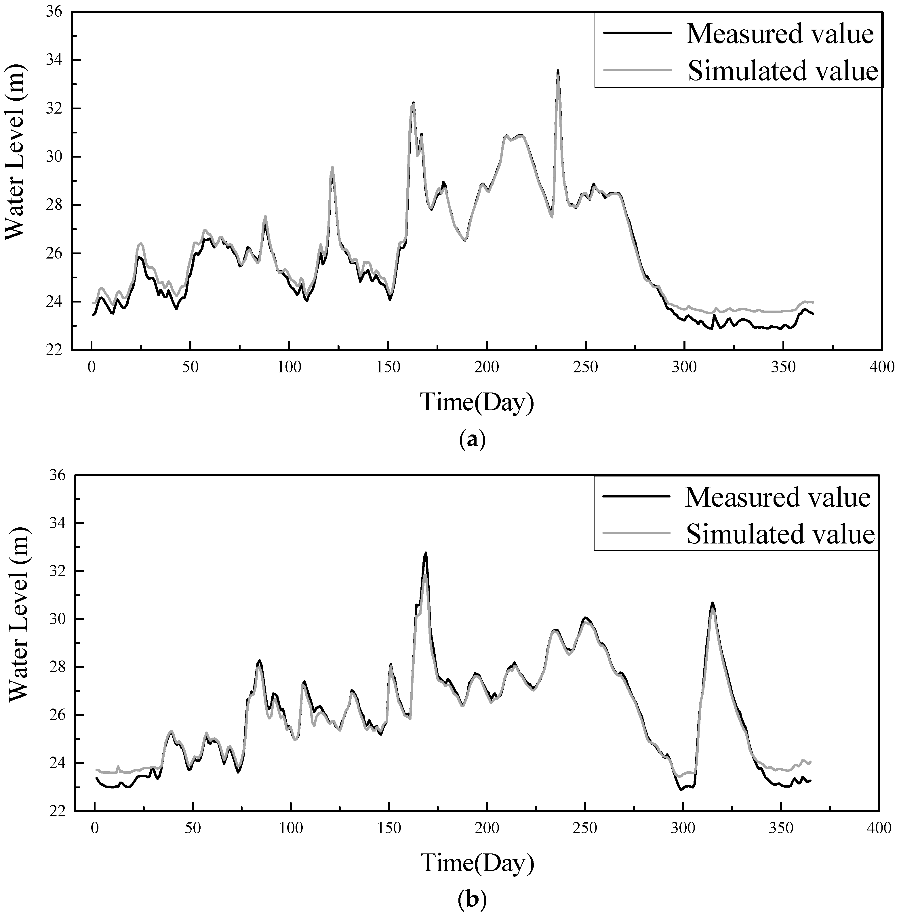
With the model parameters and boundary conditions, we constructed the hydrodynamic model using MIKE 21 module. The model was calibrated using the average daily flow and water level information at Heishipu Bridge and CCCP in 2007, and the in situ measurements using data from 2008 were for validation. Results (Figure 3) suggest that the developed model performed well in simulating water flow at the CCCP, with a relative error below 3.0%. The model performs better with a high water level and is relatively poor when the water level is low. Two factors may contribute to the discrepancy with low water levels. First, dredging activities in this reach lead to irregular shapes of riverbed with dispersed currents during the dry season, resulting in the modeled water levels being higher than the measured water levels. On the other hand, with the significant topographic variations of the riverbed, the terrain difference between the defined riverbed and the actual riverbed increases, thereby leading to modeling errors. In general, though, the estimation error is satisfactory, and the model can be employed for further simulations of the impact of water pollution incidents.

3.2. Water Pollution Accident Simulation

With the calibrated hydrodynamic model, the transport and transformation of pollutants were simulated under six different scenarios, listed in Table 1. The first three scenarios (A, B, C) were generated after the construction of the CCCP (with water level H = 29.70 m at CCCP) with different discharges at the Heishipu Bridge (Q = 2400, 1300, and 500 m³/s). The last three scenarios (D, E, F) were to simulate the water pollutant transport and transformation using natural waters (without the CCCP). 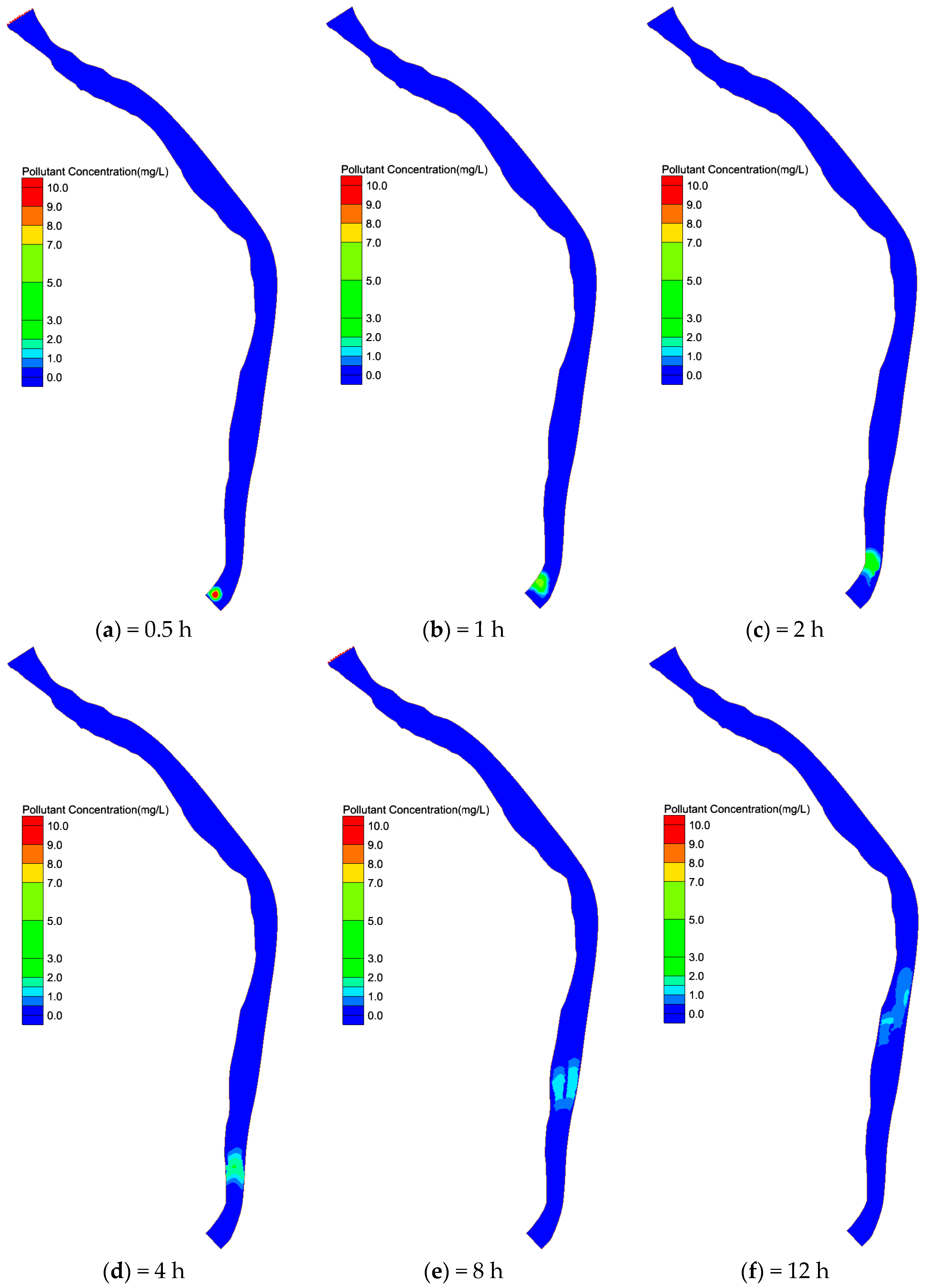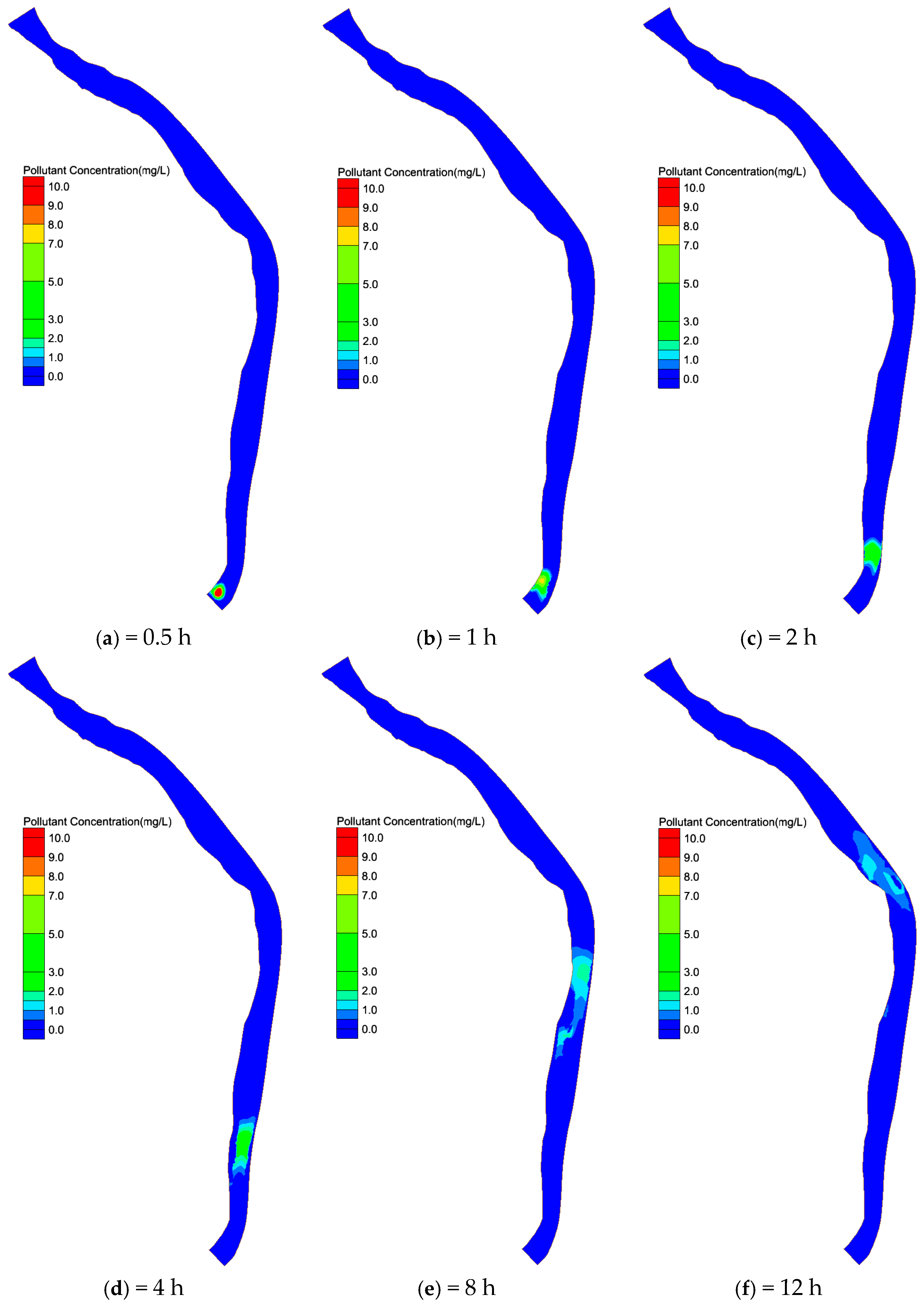With the pollutant quantity of 2600 m³ at the Heishipu Bridge, the pollutant transport and transformation temporal dynamics were obtained. As an example, Figure 4 and Figure 5 illustrate the pollutant concentration dynamics at 0.5 h, 1 h, 2 h, 4 h, 8 h, and 12 h under the scenarios A and D. Results suggest that the developed two-dimensional hydrodynamic model can clearly demonstrate the spatial–temporal trend of pollutants dynamically. This two-dimensional model is significantly better than the one-dimension model, as it can illustrate detailed information of pollutant dispersion within the river channel. As an example, under Scenario A, the simulation results show that the peak pollutant concentration is very high (approximately 10 mg/L) after 0.5 h, and this value decreases to about 7 mg/L after 1 h, 5 mg/L after 2 h, 3 mg/L after 4 h, and 1 mg/L after 8 h. Moreover, the pollutant dispersion pattern of is also very clear, and it is feasible to calculate the pollutant arrival time for a specific location, especially for waterworks intake spots. This is essential, as necessary emergency response should be taken before pollutants reach waterwork intakes.

Based on the simulation results, we calculated pollutant arrival time (see

Table 2. Pollutant arrival time at the intakes of waterworks.

Scenarios	The Second Waterworks	The Eighth Waterworks	The Third Waterworks	The First Waterworks	The Fourth Waterworks
	Arrival Time (h)	Arrival Time (h)	Arrival Time (h)	Arrival Time (h)	Arrival Time (h)
A	0.33	3.00	3.17	5.50	9.67
B	0.50	5.00	5.33	9.33	16.67
C	0.67	10.50	11.33	21.17	38.67
D	0.33	2.17	2.33	3.67	5.67
E	0.33	3.17	3.33	5.17	7.67
F	0.33	5.33	5.67	8.67	11.00

), pollutant peak concentration, and arrival time (see

Table 3. Pollutant peak concentration and arrival time at the intakes of waterworks.

Scenarios	The Second Waterworks		The Eighth Waterworks		The Third Waterworks		The First Waterworks		The Fourth Waterworks
	Peak Concentration (mg/L)	Arrival Time (h)	Peak Concentration (mg/L)	Arrival Time (h)	Peak Concentration (mg/L)	Arrival Time (h)	Peak Concentration (mg/L)	Arrival Time (h)	Peak Concentration (mg/L)	Arrival Time (h)
A	7.28	0.83	1.91	4.33	1.84	4.50	1.54	7.17	0.92	11.83
B	5.27	1.33	1.56	7.67	1.51	8.17	1.27	12.83	0.82	21.17
C	3.22	2.67	1.08	19.00	1.04	20.17	0.87	32.17	0.60	53.00
D	11.22	0.67	3.09	3.00	2.98	3.17	2.53	4.67	1.48	6.83
E	9.75	1.00	3.13	4.50	3.02	4.83	2.71	6.83	1.88	9.50
F	22.73	1.00	5.16	6.67	4.91	7.17	4.20	10.50	3.97	14.50

) for the five waterworks along the reach, including the Second Waterworks, the Eighth Waterworks, the Third Waterworks, the First Waterworks, and the Fourth Waterworks, sequentially, following the river direction (Figure 6). Table 2 indicates that the arrival time is positively associated with the distance from the Heishipu Bridge for each scenario. As an example, under Scenario A, the pollutant reaches the Second Waterworks after 0.33 h, the Eighth Waterworks after 3 h, the Third Waterworks after 3.17 h, the First Waterworks after 5.5 h, and the Fourth Waterworks after 9.67 h. Similarly, Table 3 indicates a decreasing trend of pollutant peak concentrations of waterworks from upstream to downstream. Taking Scenario A as an example, the pollutant arrives at the Second Waterworks with a peak concentration of 7.28 mg/L, at the Eighth Waterworks with a peak concentration of 1.91 mg/L, at the Third Waterworks with a peak concentration of 1.84 mg/L, at the first Waterworks with a peak concentration of 1.54 mg/L, and finally at the Fourth Waterworks with a peak concentration of 0.92 mg/L.

In addition to the general trend of pollutant dispersion, we also performed comparative analyses of different scenarios to examine (1) the impact of the CCCP on the pollutant arrival times and concentrations; (2) the impact of discharges under CCCP scenarios; and (3) the impact of discharges with the natural water scenarios.

• Impact of CCCP on the pollutant arrival time and concentration.
  As shown in Figure 6, it can be discerned that the CCCP has a significant impact on the dispersion of the pollutant. Taking Scenarios A (with CCCP) and D (without CCCP) as examples, with the same discharge (e.g., 2400 m³/s), it takes a much longer time for the pollutant to reach the intakes of each waterworks, and the peak concentration of the pollutant is much lower. As an example, under Scenario A, it takes approximately 4.33 h (with a peak concentration of 1.84 mg/L) for the pollutants to reach the Third Waterworks, while it only takes 3.17 h (with a peak concentration of 2.98 mg/L) under Scenario D. Similar patterns can be discerned with different discharges (e.g., when comparing B and E, and C and F). This result is unsurprising, as the water level in the downstream is significantly higher due to the construction of the CCCP, which subsequently leads to decreased water velocity. Therefore, the transport velocity of pollutant is decreased, and the pollutant is diluted and dispersed in all directions.
• Impact of discharge under CCCP scenarios.
  Figure 7 shows the pollutant concentration characteristics with different discharges (e.g., 2400 m³/s, 1300 m³/s, and 500 m³/s) under CCCP scenarios (e.g., water level is 29.7 m). Comparative analysis indicates that, when discharge decreases, the arrival time to waterworks intakes increases with decreased pollution concentration. Taking the Eighth Waterworks as an example, the arrival time of pollutant is 3 h with a peak concentration of 1.91 mg/L with the discharge of 2400 m³/s; the arrival time increases to 5 h with a peak concentration of 1.56 mg/L when the discharge decreases to 1300 m³/s; and, finally, the arrival time increases to 10.5 h with a peak concentration of 1.08 mg when the discharge further decreases to 500 m³/s. As a summary, under CCCP scenarios, with the same downstream water level (29.70 m), discharge at the upstream is negatively associated with the arrival time and positively associated with the peak concentrations of each waterwork intake. This result is reasonable, as the higher value of discharges leads to a higher velocity of pollutant transport, and a higher pollutant concentration.
• Impact of discharge with the natural water scenarios.
  Under the natural water scenarios, the impacts of different discharges on pollutant transport are shown in Figure 8. Comparative analyses suggest that, when discharge decreases, the arrival time to waterwork intakes increases, although with increased pollution concentrations. Taking the Eighth Waterworks as an example, the arrival time of the pollutant is 2.17 h with a peak concentration of 3.09 mg/L when the discharge is 2400 m³/s; the arrival time increases to 3.17 h with a peak concentration of 3.13 mg/L when the discharge decreases to 1300 m³/s; and, finally, the arrival time increases to 5.33 h with a peak concentration of 5.33 mg when the discharge further decreases to 500 m³/s. As a summary, under the natural water scenarios, discharge is negatively associated with the arrival time, as well as the peak concentrations of each waterworks’ intake. This result is likely be explained by the water quantity within the reach. That is, under natural water conditions, lower discharge in the dry season is associated with lower water quantity, thereby leading to higher peak pollutant concentrations.

4. Discussion

To understand the mechanism of the transport and transformation of pollutants in a river system, this study developed a hydrodynamic model based on the convective diffusion module of MIKE21 and simulated the pollutant transport under different scenarios based on the options of discharge and the construction of the CCCP. Two fundamental questions have been answered through this simulation: (1) When will the pollutants arrive at a given point (e.g., waterwork intakes)? (2) What are the peak pollutant concentrations (and when) for a given point?

Comparative analyses suggest that the CCCP plays a central role in the process of pollutant transport. With the CCCP, it takes a longer time for the pollutants to reach a waterwork intake, and the pollutant concentration is also much lower for all scenarios. This is expected; as the water level at the CCCP is raised to a normal water level (29.70 m in this study), the velocity of the water (and pollutants) decreases significantly, which subsequently leads to a longer pollutant arrival time for a specific spot, and a lower peak pollutant concentration due to dispersion.

The analyses associated with upstream discharge also suggest the importance of the CCCP. Although a general pattern that higher discharges will lead to shorter arrival times can be discerned for all scenarios, a contradictory trend of peak pollutant concentration with CCCP and without CCCP has been found. That is, with the CCCP, lower discharge leads to lower peak pollutant concentration, while, without the CCCP, lower discharge leads to higher peak pollutant concentration. This difference can be explained by the water quantity within the reach. Therefore, with the CCCP, the water quantity does not vary significantly, as the water level of the downstream has been set to 29.7 m. Under the natural condition, however, the water quantity has been significantly reduced during dry season; moreover, with a lower discharge at the upstream, the peak pollutant concentration is higher, largely due to lower water quantity. As a result, the role of the CCCP in alleviating water pollution is more significant with lower upstream discharges (e.g., during the dry season).

While this simulation model has satisfactorily examined the role of the CCCP dam on the transport and transformation of pollutants resulted from a water pollution accident, a real-world pollutant transport analysis is essential for model validation. In this study, however, we could not perform such an analysis due to the lack of in situ measurement data, and the scarcity of water pollution incidents. Real-world measurements and analyses, however, are essential for a better understanding of the pollutant transport and transformation processes within a river system. For the generation of the simulation model, we did not consider a number of factors that may impact pollutant transport and transformation. For example, we did not incorporate water degradation values into the analyses. For a particular water pollution accident, it is necessary to consider the effect of pollutant degradation. In addition, we did not consider the impact of effluents. Within this reach, no major effluents could be found, and this omission should not significantly affect our results. In future research, it may be necessary to consider more factors in order to build a more realistic model.

5. Conclusions

This paper constructed a hydraulic water quality model to simulate the transport and transformation of pollutants caused by water pollution incidents using the hydrodynamic module and convective diffusion module of MIKE21. Six scenarios, three after the construction of the CCCP and three under natural conditions, were built in order to examine the transport and transformation processes of pollutants. Especially, the spatio–temporal dynamics of pollutant distribution, as well as the arrival times and peak concentrations at waterwork intakes, were simulated and analyzed. Analysis of the results suggests two major conclusions.

First, the CCCP plays a central role in controlling the transport and transformation of pollutants. After the construction of the CCCP, the water level in the downstream area is raised, therefore reducing the velocity of water and pollutants. As a result, the process of transport is weakened, and the dispersion effect is strengthened. Therefore, the arrival time of the pollutants at each waterwork intake becomes longer with a decreased peak pollution concentration. Therefore, the construction of the CCCP reduces the adverse effect of pollutants on human beings and natural environments.

Second, although, in general, the CCCP serves a role in reducing pollutant concentrations and increasing the pollutant arrival time for each waterwork intake, such a function is more significant with lower discharges (e.g., during the dry season), largely due to the higher amount of water quantity within the reach with the CCCP.

References

- Meng, W. How to deal with abrupt water pollution accident. World Environ. 2009, 2, 30–31. (In Chinese) [Google Scholar]
- Zhang, B.; Qin, Y.; Huang, M.; Sun, Q.; Li, S.; Wang, L.; Yu, C. SD–GIS-Based temporal–spatial simulation of water quality in sudden water pollution incidents. Comput. Geosci. 2011, 37, 874–882. [Google Scholar] [CrossRef]
- Yu, S. It is urgent to prevent water pollution. J. Chem. Ind. Manag. 2014, 25, 32–33. (In Chinese) [Google Scholar]
- He, Q.; Peng, S.; Zhai, J.; Xiao, H. Development and application of a water pollution emergency response system, for the Three Gorges Reservoir in the Yangtze River, China. J. Environ. Sci.-China 2011, 23, 595–600. [Google Scholar] [CrossRef]
- Streeter, H.W.; Phelps, E.B. A Study of the Pollution and Natural Purification of the Ohio River. Arch. Biochem. 1925, 18, 69–83. [Google Scholar]
- Cox, B.A. A review of currently available in-stream water-quality models and their applicability for simulating dissolved oxygen in lowland rivers. Sci. Total Environ. 2003, 314–316, 335–377. [Google Scholar] [CrossRef]
- Salterain, A.; Sancho, L.; Rodrigues, E.; Pinilla, L.; Ayesa, E. Development and verification of a new simulation tool for water quality prediction in the Ebro river progress in water resources. Water Pollut. VII Model. Meas. Predict. 2003, 9, 13–22. [Google Scholar]
- Hu, H.; Huang, G. Monitoring of Non-Point Source Pollutions from an Agriculture Watershed in South China. Water 2014, 6, 3828–3840. [Google Scholar] [CrossRef]
- Li, Y.; Yao, J. Estimation of Transport Trajectory and Residence Time in Large River–Lake Systems: Application to Poyang Lake (China) Using a Combined Model Approach. Water 2015, 7, 5203–5223. [Google Scholar] [CrossRef]
- Wang, Q.; Zhao, X.; Wu, W. Advection-Diffusion models establishment of water-pollution accident in middle and lower reaches of Hanjiang River. Adv. Water Sci. 2008, 19, 500–504. [Google Scholar]
- Gao, Q.; Li, Y.; Cheng, Q.; Yu, M.; Hu, B.; Wang, Z.; Yu, Z. Analysis and assessment of the nutrients, biochemical indexes and heavy metals in the Three Gorges Reservoir, China, from 2008 to 2013. Water Res. 2016, 92, 262–274. [Google Scholar] [CrossRef]
- Zhang, Y.; Xia, J.; Liang, T.; Shao, Q. Impact of water projects on river flow regimes and water quality in Huai River Basin. Water Resour. Manag. 2010, 24, 889–908. [Google Scholar] [CrossRef]
- Santucci, V.J., Jr.; Gephard, S.R.; Pescitelli, S.M. Effects of multiple low-head dams on fish, macroinvertebrates, habitat, and water quality in the Fox River, Illinois. N. Am. J. Fish. Manag. 2005, 25, 975–992. [Google Scholar] [CrossRef]
- Wei, G.; Yang, Z.; Cui, B.; Li, B.; Chen, H.; Bai, J.; Dong, S. Impact of dam construction on water quality and water self-purification capacity of the Lancang River, China. Water Resour. Manag. 2009, 23, 1763–1780. [Google Scholar] [CrossRef]
- Crabtree, B.; Earp, W.; Whalley, P. A demonstration of the benefits of integrated wastewater planning for controlling transient pollution. Water Sci. Technol. 1996, 33, 209–218. [Google Scholar] [CrossRef]
© 2016 by the authors; licensee MDPI, Basel, Switzerland. This article is an open access article distributed under the terms and conditions of the Creative Commons Attribution (CC-BY) license (http://creativecommons.org/licenses/by/4.0/).