Uncertainty Analysis in Data-Scarce Urban Catchments

Abstract

The evaluation of the uncertainties in model predictions is key for advancing urban drainage modelling practice. This paper investigates, for the first time in Mexico, the effect of parameter sensitivity and predictive uncertainty in an application of a well-known urban stormwater model. Two of the most common methods used for assessing hydrological model parameter uncertainties are used: the Generalised Likelihood Uncertainty Estimation (GLUE) and a multialgorithm, genetically adaptive multi-objective method (AMALGAM). The uncertainty is estimated from eight selected hydrologic parameters used in the setup of the rainfall-runoff model. To ensure the reliability of the model, four rainfall events varying from 20 mm to 120 mm from minor to major count classes were selected. The results show that, for the selected storms, both techniques generate results with similar effectiveness, as measured using well-known error metrics; GLUE was found to have a slightly better performance compared to AMALGAM. In particular, it was demonstrated that it is possible to obtain reliable models with an index of agreement (IAd) greater than 60 and average Absolute Percentage Error (EAP) less than 30 percent derived from the uncertainty analysis. Thus, the quantification of uncertainty enables the generation of more reliable flow predictions. Moreover, these methods show the impact of aggregation of errors arising from different sources, minimising the amount of subjectivity associated with the model’s predictions.

1. Introduction

Recently, hydrological modelling has become more relevant, based on the technological advances that provide better spatial and temporal resolution. However, the ability to incorporate spatially distributed digital data is in turn hindered by the scarcity of datasets at the same scale. Alternatively, remote sensing techniques make it possible to rapidly obtain information for large areas by means of sensors operating in several spectral bands, mounted on aircraft or in satellites [1,2]. The above-described situation has opened the door to the use of big data [3], applying it to hydrological models to make them more robust. Nevertheless, modelling spatially distributed hydrological processes can be challenging, particularly in strongly heterogeneous (soil use variation, slope, coverage) urbanised areas. Multiple interactions occur in urban areas between structures and the drainage system (for waste water and storm water) at various temporal and spatial scales, which in turn increase the data requirements and complexity [4]. These complexities, in addition to the aforementioned data scarcity at the required level, make it difficult to define a universal methodology to reproduce urban flows at the catchment scale. Therefore, there is a growing need to assess the effect of uncertainty in results derived from hydrologic modelling approaches utilised in urban environments [5,6].

Models of hydrological processes produced by previous researchers incorporate uncertainty from a variety of sources. This uncertainty can lead to unrealistic results because of the interaction and aggregation of known and unknown errors within the modelling process [7]. Research must be performed to estimate these errors [8,9]. It is acknowledged that knowing the factors that cause the uncertainty and its propagation in the final results will facilitate reliable hydrological modelling that can be used in decision making, structure design, flood warnings and emergency actions in urban environments, see [10].

The sources of uncertainty can be categorised as either aleatory or epistemic [11]. On one hand, aleatory uncertainty is caused by random or stochastic characteristics of natural processes that are variable over space and time (e.g., soil moisture); such uncertainty is not reducible. On the other hand, epistemic uncertainty is error caused by poor measurement, lack of knowledge, and exclusion of the processes by poor representation in a hydrologic model. Most of the epistemic uncertainty can be addressed by increasing information and improving data quality, except those that arise from the ‘unknown unknowns’, which are irreducible [12].

Moreover, there is also uncertainty associated with input data in the models, for example rainfall, land cover, and soil hydraulic properties [13]. The accurate representation of the spatio-temporal variability of these quantities in the field represents a particular challenge for catchments where the information of the gauge networks is sparse [14]. In addition, there is uncertainty in the observed data that is used for model calibration, as possible errors could arise from the measurement of flow velocity and water depth, backwater effect, changes in river cross sections and fitting rating curve.

Model structure uncertainty (uncertainty in the parameter definition) is recognised as a main contributor to model prediction uncertainty; however, it is often ignored [15]. Model structure uncertainty can be reduced if the dominant processes are sufficiently represented [16]; however, it cannot be completely eliminated, even if the input data are error-free, because catchment responses are averaged over space and time [17].

The influence of model structure uncertainty is exacerbated in catchments where knowledge of the dominant processes is limited and the choice of model structure is restricted by data availability. In data scarce catchments, model structure uncertainty is addressed by incorporating model structure into parameter uncertainty, which may be achieved by an analysis of the regression residuals between model predictions and observations [18]. However, the problem of reducing model parameter uncertainty is further complicated by interactions between parameters, leading to difficulties in identifying optimal parameter values. Equifinality is considered as different combinations of parameter values that have performed equally well in terms of the selected objective functions [19,20,21,22].

Evaluation of the uncertainty in predictions from hydrological models applied to urban catchments has been limited [23,24]; as a consequence, such evaluations have not been widely used in engineering practice. In this sense, the transference between the knowledge fields of different uncertainty analysis approaches is required for the uncertainty characterisation in the hydrological modelling of urban basins [25].

Among the most widely used uncertainty analysis techniques are the Generalised Likelihood Uncertainty Estimation (GLUE) approach [11], the classical Bayesian Monte Carlo (i.e., Bayesian inference approach) [23] and those that include the optimisation algorithms SCEM-UA [26,27] and AMALGAM [28].

Following [29], GLUE ‘‘represents an extension of Bayesian or fuzzy averaging procedures to less formal likelihood or fuzzy measures.” The concept of ‘‘the less formal likelihood” represents the main element of differentiation with the Bayesian inference. Although Bayesian methods present a formal statistical framework to the treatment of parameter distributions, they require a large amount of data, making their implementation difficult in data scarce applications. In comparison with Bayesian methods, the GLUE method is easy to implement. Some researchers have adopted these methodologies for performing the uncertainty analysis of model parameters. For example, in the case of [30], the wetland design parameters for flooding control relating the hydrological and hydraulical parameters were analysed for a better model performance. Another example is the work of Fraga et al. [31], in which the model parameter uncertainty and its propagation from a hydrological model 1D-2D was evaluated. Similarly, the work of Sun et al. [32] focused on the hydrological parameters uncertainty behaviour regarding the model scale (surface study detail), and the work of Zhao et al. [33] involved an uncertainty analysis for evaluating the capability of different likelihood measures in model parameter distribution.

Because data are scarce in much of the world (especially in developing countries), the focus of research should be on the reduction of the predictive uncertainty by achieving a better understanding of processes and the quantification of uncertainty itself [34,35]. This can be achieved through a comparison of the different approaches in data-scarce regions.

This investigation presents a comparison of two of the most common methods used for assessing hydrological model parameter uncertainties in an urban catchment in Mexico. The methods compared are (a) the Generalised Likelihood Uncertainty Estimation (GLUE) developed by [11]; and (b) a multialgorithm, genetically adaptive multi-objective method (AMALGAM) developed by Vrugt and Robinson [36]. The comparison aims to show the performance of both methods in implementing a well-known open-source model (Storm Water Management Model, SWMM) in a small urban catchment, using the index of agreements as the likelihood measure. In this case, the quantification of the uncertainty is estimated from the hydrologic parameters used in the setup of the rainfall-runoff model. This application will show the advantages of implementing such an analysis in applications with limited data.

The paper is organised as follows: Section 2 illustrates the performance methodology implemented for the comparison; Section 3 presents the case study along with the available data and the methods implemented; and Section 4 summarises the results and discussions. Finally, Section 5 introduces the main conclusions derived from this work.

2. Methodology

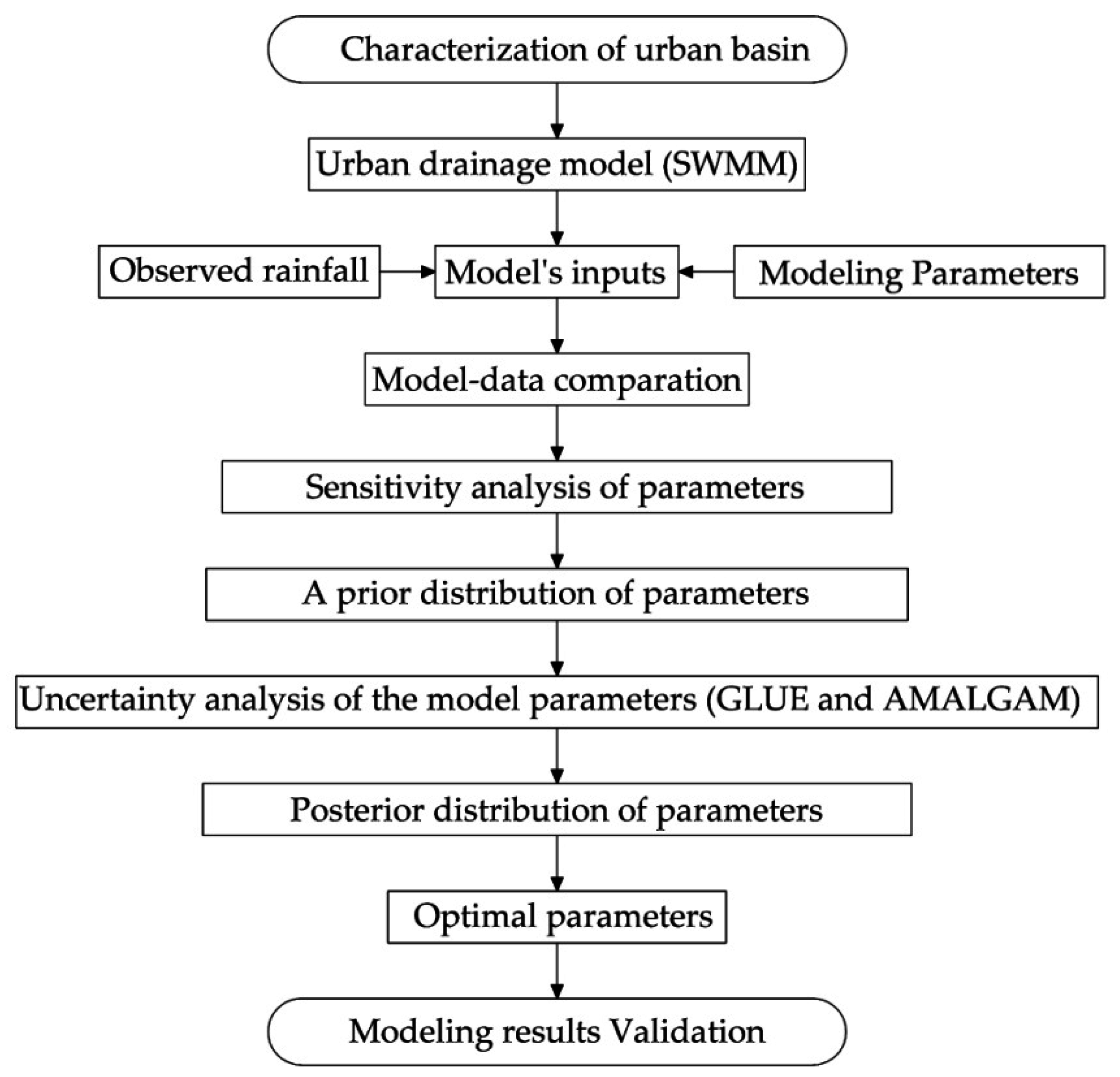
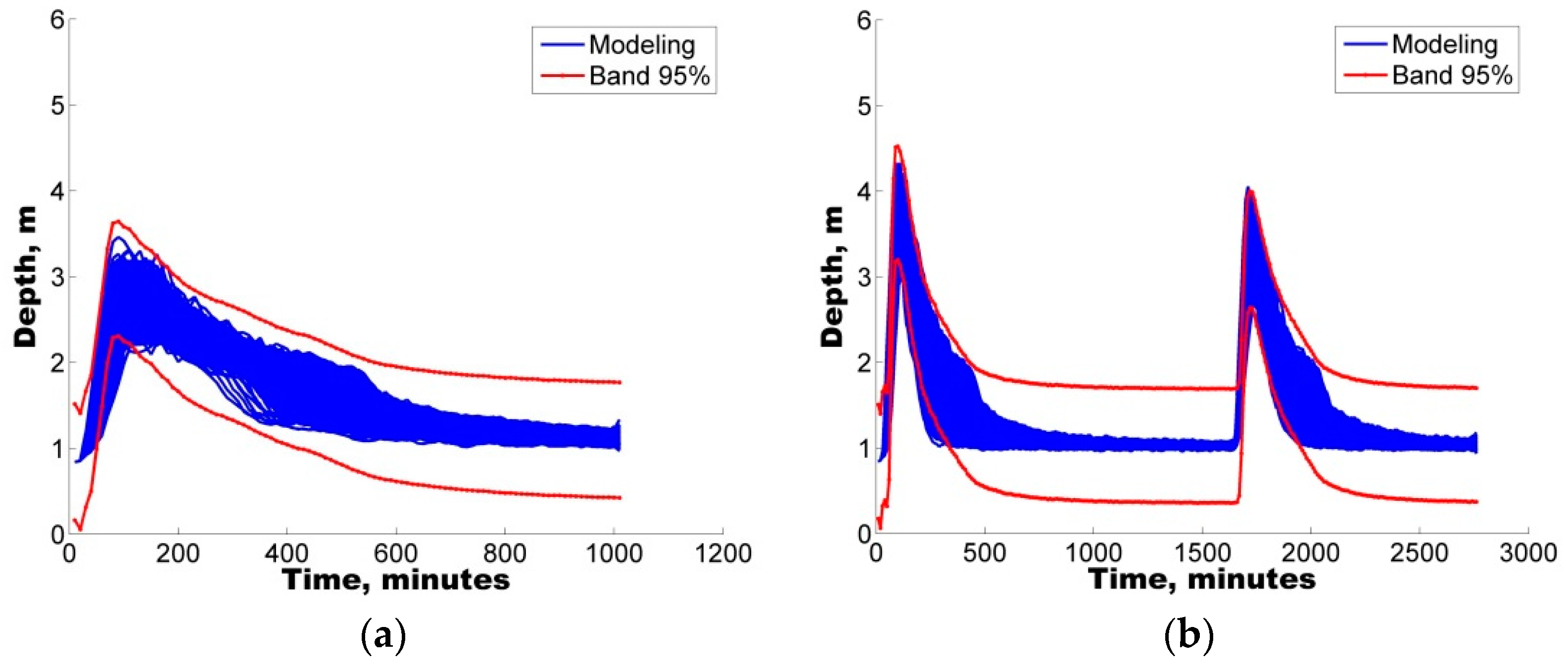
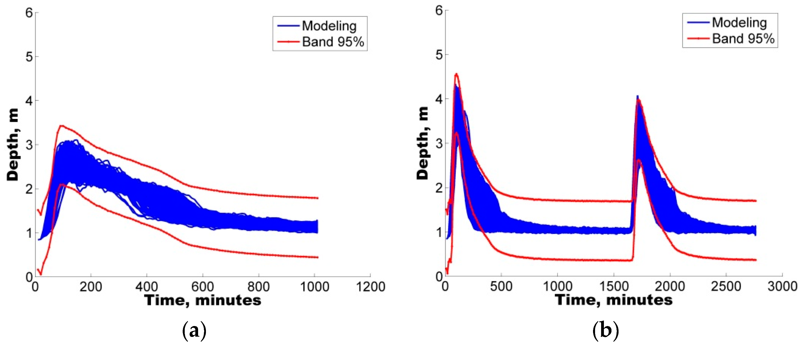
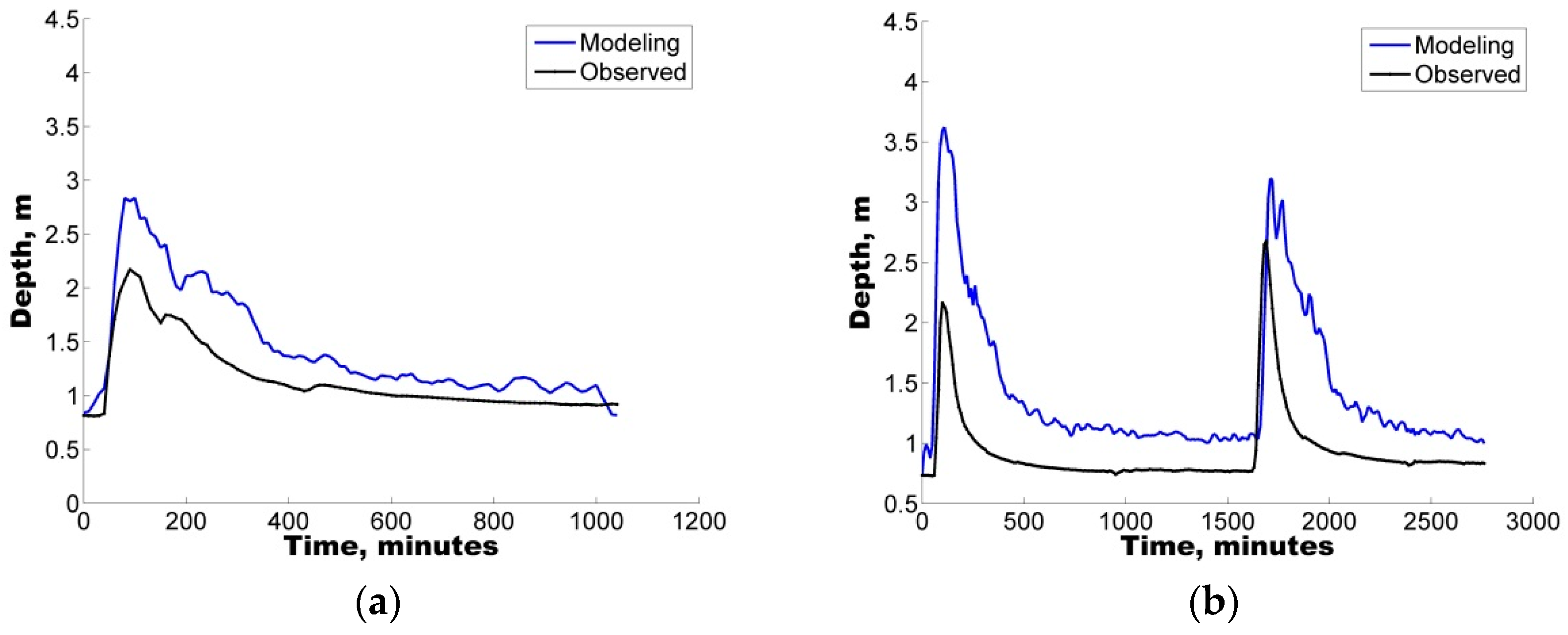
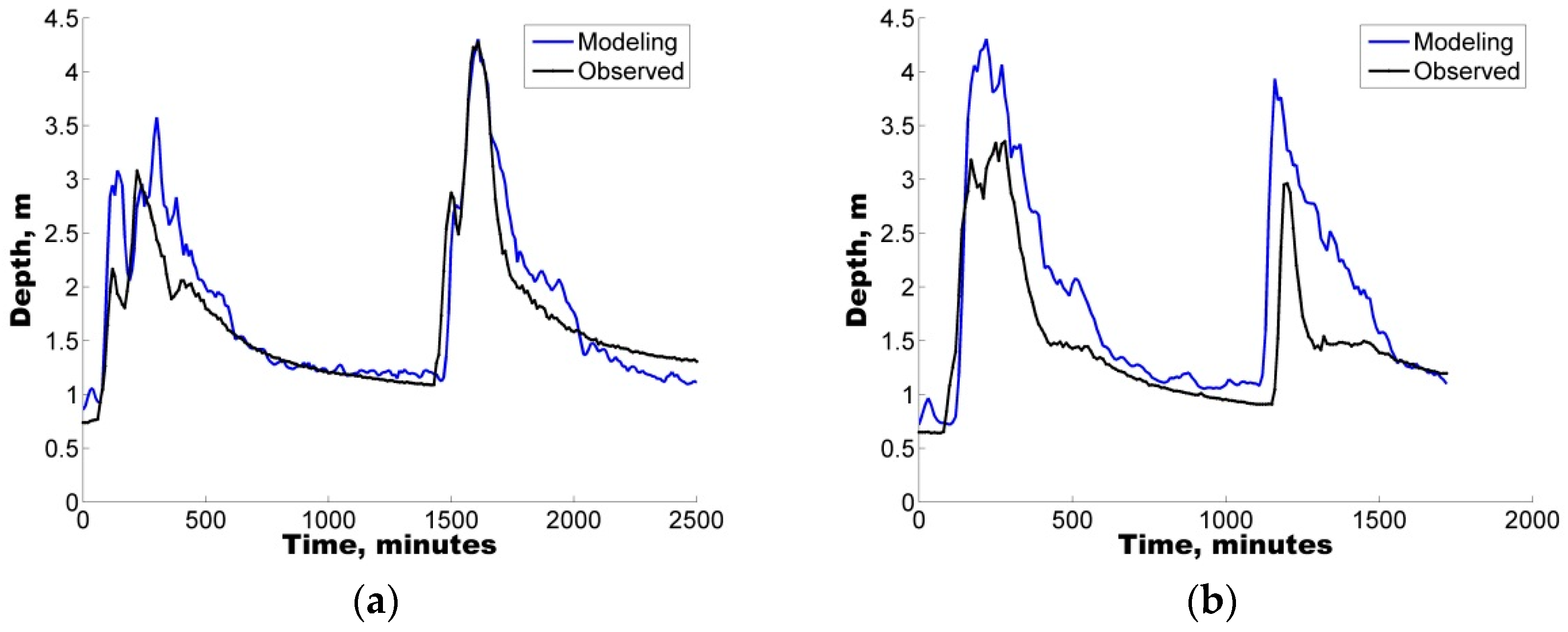
A flow chart of the methodology (shown in Figure 1) illustrates the uncertainty analysis process, which involves the characterisation of the basin, followed by the hydrologic modelling and model-data comparison at the selected gauging station. Modelling errors for each run are evaluated and selected or discarded in relation to the defined confidence envelope. The uncertainty analysis techniques of GLUE and AMALGAM were used to quantify the uncertainties derived from the selected parameter sets. Following the work presented by Dotto et al. [37], the results are evaluated through a measure of the model run performance through the index of agreement (IAd) and the Average Relative Interval Length (ARIL) [38] (see Equation (1)), complemented with the evaluation of the Absolute Percentage Error (APE) (see Equation (2)). The set of “best” parameters is estimated based on the results that are within the range of 95% confidence. The ARIL coefficient is specified as follows:

$$\mathrm{ARIL}=\frac{1}{N}{\displaystyle \sum }_{i=1}^N\frac{{\mathit{Limit}}_{\mathit{upper},i}-{\mathit{Limit}}_{\mathit{lower},i}}{X_{\mathit{obs},i}}$$

(1)

where $N$ is the number of results within the confidence band, ${\mathit{Limit}}_{\mathit{upper},i}$ is the upper limit of the confidence band, ${\mathit{Limit}}_{\mathit{lower},i}$, is the lower limit of the confidence band, and $X_{\mathit{obs},i}$, is the observed value at the instant i within the confidence band.

$$\mathrm{APE}=\left|\frac{D_i-O_i}{O_i}\right|\times 100$$

(2)

where $D_i$ is the model result, and $O_i$, is the observed value at the same instant i.

This comparison procedure between the two implemented uncertainty techniques was determined following the criteria proposed in previous investigations [39,40], where the performance of the model is assessed by the IAd proposed by Willmot [41] and used by Krause et al. [42] as a measure for the likelihood (Equation (3)), and the model prediction uncertainty is defined through the ARIL 95% probability bands (as proposed by Jin et al. [38]).

$$\mathrm{IAd}=1-\frac{{\displaystyle {\sum }_{i=1}^n{\left(O_i-D_i\right)}^2}}{{\displaystyle {\sum }_{i=1}^n}{(|D_i-\overline{O}|+|O_i-\overline{O}|)}^2}$$

(3)

where $D_i$ is the modelling result in the instant i, $O_i$, is the observed value in the instant i and $\overline{O}$ is the observed average.

3. Study Area, Hydrological Model and Uncertainty Methods

3.1. Study Area

The city of Tuxtla Gutierrez, located in the Mexican state of Chiapas, Mexico, was selected as the case of study. The population is approximately 553,374. The average elevation of Tuxtla Gutierrez is 600 m above the mean sea level, and the average annual temperature is 25.4 °C. The climate is influenced by an intense wet season in combination with the incidence of hurricanes and cold fronts. The relative humidity fluctuates between 80% and 86%, and the annual rainfall is 956 mm, mainly between May and October. The city is located within the catchment of the Sabinal River (see panel a Figure 2); its main channel crosses the city along 21 km from West to East. The catchment area of 407 km² was instrumented with seven automatic weather stations, each of which measured climatic parameters with a temporal resolution of 10 min.

Four storm events from 2011 were selected because they induced flooding, which is the principal problem in the study basin. Figure 2b–e illustrates the hyetographs for each event registered at the seven weather stations, where differences in the registered rainfall at these points are shown for some cases. In addition, these events have the same temporal resolution as the hydrometrical stations, 10 min, thereby enabling calibration of the rain runoff model in the basin; thus, events one and two are used in the uncertainty analysis and events three and four are used in its validation. The gauging station closer to the catchment exit point (triangle No. 5 in Figure 2) is used to compare the rainfall-runoff model results. The measured discharge at this point is depicted in Figure 2f, showing records from 1 July 2011 to 31 October 2011. The selection of station five and the register period was due to the lack of reliable information in the other measurement points; as a result, they were not possible to use in the uncertainty analysis.

3.2. Hydrological Model

The computational model used in this study was the Storm Water Management Model (SWMM) produced by the Environment Protection Agency of the United States [43]. SWMM is a dynamic hydrology-hydraulic water quality simulation model that can be used for single event or long-term (continuous) simulation of runoff quantity and quality from primarily urban areas. The runoff component operates on a collection of sub-catchment areas that receive precipitation and generate runoff. The version used in this study was SWMM 5.0.022.

SWMM estimates the runoff by considering each one of the sub-basins as a nonlinear reservoir, where the contribution of flow to the deposits comes from precipitation, snow, or releases from upstream stores. SWMM also simulates route flows from the system, infiltration, evaporation and surface runoff. The surface runoff of a given area is determined when the water depth within a catchment exceeds the maximum storage value, and the outflow is determined by Manning (5) or Hazen-Williams Equation (6), which integrates the continuity Equation (4) considering friction through the incorporation of Manning coefficient (n). The major loss considered in the rainfall and runoff modelling is infiltration loss, which is calculated through either Horton (7), Green Ampt (8) or (9) and Soil Conservation Service (SCS) curve number. The infiltration losses are considered only from the pervious areas of a sub-catchment. The Horton model was selected for this study. Implemented variables in the SWMM model are presented below, and

Table 1. Range parameters and the initial values for modelling.

Parameter	Abbreviation	Minimum Value	Maximum Value	Initial Value
Manning coefficient n conduit	ManN	0.01	0.03	0.065
Manning coefficient n impermeable surface	Nimperv	0.001	0.2	0.01
Manning coefficient n permeable surface	Nperv	0.01	0.2	0.1
Height depression storage on the impermeable area, $\mathrm{mm}$	Simperv	0	10	5
Height depression storage on the permeable area, $\mathrm{mm}$	Sperv	0	20	1.27
Percent impermeable area without storage in the depression, $\text{\%}$	PctZero	0	100	25
Maximum rate of infiltration, $\mathrm{mm}/\mathrm{h}$	MaxRate	1	200	11.7
Minimum rate of infiltration, $\mathrm{mm}/\mathrm{h}$	MinRate	1	25	5.6
Decay coefficient, $\mathrm{L}/\mathrm{h}$	Decayk	1	30	4

introduces the parameters used in this study with the different uncertainty analysis techniques. These are shown along with the application ranges that are defined using Kalimod v3.0 [44].

$$A\frac{\partial y}{\partial t}=Ai-Q$$

(4)

where $A$ is the basin area, $y$, the water depth, $t$, the time, $i$, the rainfall intensity and $Q$ the flow.

$$Q_M=\frac{1}{n}L{\left(y-y^{\prime }\right)}^{5/3}{S}^{1/2}$$

(5)

where $Q_M$ is the flow by Manning, $n$, the Manning coefficient, $L$, the width sub-basin, $y$, the water depth, $y^{\prime }$, the lowering of height storage and $S$ the slope.

$$Q_{H-W}=1.318{CAR}^{0.63}{S}^{0.54}$$

(6)

where $Q_{H-W}$ is the flow by Hazen-Williams, C, the Hazen-Williams roughness, $A$, the area, $R$, the hydraulic radius and $S$ the slope.

$$f_p=f_o-\left(f_o-f_{\infty }\right){\mathrm{e}}^{-{\propto }_d\left(t-t_w\right)}$$

(7)

where $f_p$ is the soil infiltration capacity, $f_{\infty }$, the minimum or end value of $f_p$ $\left(\mathit{in}t=\infty \right)$, $f_o$, the maximum or initial value of $f_p$ $\left(\mathit{in}t=0\right)$, $t_w$, the start time of the storm and ${\propto }_d$, decay coefficient.

$$F_s=\frac{S_{u}IMD}{i/K_s-1}\mathrm{for}i>K_s;f=i$$

(8)

$$f_p=K_s\left(1+\frac{S_{u}IMD}{F}\right)\mathrm{for}i\le K_s;f=f_p$$

(9)

where $F_s$ is the cumulative infiltration volume required to cause surface saturation, $F$, the cumulative infiltration volume, $f_p$, the soil infiltration capacity, $f$, the infiltration rate, $K_s$, the hydraulic conductivity of soil saturation, $i$, the rainfall intensity, $S_u$, is the average capillary suction in the wetting front and $IMD$, is the initial moisture deficit of the event.

3.3. Sensitivity Analysis

A sensitivity analysis was conducted through the range of values that are valid for each of the parameters in the model conducted during the application of the selected uncertainty analysis techniques. A Monte Carlo sampling method was implemented, for this purpose, which considered 1000 random samples of possible values for each model parameter and a uniform probability distribution (similar to [11]). For each model parameter, the sensitivity coefficient is calculated according to the following [45], Equation (10):

$$s_{i,j}=\frac{{\mathrm{\Delta }\mathsf{\theta }}_j}{{\mathit{ys}}_i}\frac{\partial y_i}{\partial {\mathsf{\theta }}_j}$$

(10)

where $y_i$ represents the n model output variables, ${\mathsf{\theta }}_j$ represents the m independent model parameters, ${\mathrm{\Delta }\mathsf{\theta }}_j$ represents the j-th parameter variability range and $y{s}_i$, is the reference value (or scaling) for the variable $y_i$ used to preserve the non-dimensional nature of the sensitivity function.

3.4. Uncertainty Analysis Techniques

Following the local sensitivity analysis, the uncertainty analysis techniques are applied by considering only the simultaneous variation of sensitive parameters and keeping the others constant with their calibration values. The model parameters used for the uncertainty analysis are presented in Table 1.

3.4.1. GLUE Methodology

GLUE methodology considers a range of parameter sets that provide reliable simulation results when compared with a single observation, thus transforming the problem to a search for sets of parameter values that are valid (e.g., equifinality). The advantage of this technique is that there is no requirement for detailed distribution functions of the observable variables/errors when the number of parameters is high or the data are limited [46].

However, when data availability is not a problem, such a methodology may use subjective hypotheses in the selection of the threshold acceptance of the parameters sets that can adjust the model (e.g., [47]). The GLUE technique [11] relies solely on the measure of performance of different sets of parameters that are derived from the application of indices that measure their skill to represent the best adjustment of a model’s results (e.g., the likelihood and probability of the model result based on the parameter set) and does not involve the minimisation or maximisation of an objective function. In this study, IAd is implemented as a performance measure.

3.4.2. AMALGAM Method

The Adaptive Multi Algorithm Genetically Multi-objective method (AMALGAM) was developed to solve problems in the meteorological predictions field. The method combines two concepts, the search with simultaneous methods and the auto-evolutionary descendent creation, which guarantee fast, reliable and computationally efficient solutions in the multi-objective optimisation algorithms setting.

The multi-evolutionary optimisation method implements an elitist search procedure based on the population, which has characteristics of the set of distributed parameters with Pareto solutions, in a single optimisation procedure [36,48]. AMALGAM uses for optimisation the algorithms listed below:

• Non-dominated sorted genetic algorithm-I I (NSGAII) [49].
• Particle swarm optimisation (PSO) [50].
• Adaptive Metropolis search (AMS) [51].
• Differential Evolution (DE) [52].

In this study, the implementation of this algorithm is conducted through the utilisation of the KALIMOD software tool [44], which was developed as an interface between simulation models and optimisation algorithms. The general procedure involves the selection of relevant rainfall-runoff events to perform multi-event calibration with AMALGAM.

4. Results and Discussion

4.1. Model-Data Comparison

The first step in the methodology involved the model data comparison (at gauging station No. 5) for the selected catchment. In this case, once the hydraulic model has been established through the characterisation of the catchment, the two selected storm events are reproduced using optimal values for the free parameters in the model. This model-data comparison is illustrated in Figure 3 for the two selected events in this study. Panel a shows that, in the case of the first event, the hydraulic model overestimates the measured level in the river. The average absolute percentage error for the entire hydrograph was estimated as 28.40%, with a maximum value of 114.25% close to the peak discharge. Panel b introduces the same result for the second storm, also overestimating the river level. In this case, the average absolute percentage error was estimated as 44.01% for the entire record, with maximum errors of 323.13% in the peak discharge.

From these results, it is again clear that errors behave differently for each storm event, highlighting the great need in such cases to incorporate a sensitivity analysis of the hydrologic parameters involved. Therefore, following this result, the implementation of two different uncertainty techniques was conducted.

4.2. Sensitivity Analysis

The sensitivity analysis is performed for selected parameters in the hydrological model; these parameters are reported in Table 1, along with the maximum and minimum values established for the analysis.

Because of the influence in the runoff hydrographs generation (extension, size and shape) nine parameters of the sensibility analysis were selected. Furthermore, the relationship between the parameters (according to the type of surface and the storage) and the infiltration rate generating the urban basin runoff is determined. The results illustrated in Figure 4 indicate that the Manning coefficient, n, of the impervious surface (Nimperv) is the most sensitive to changes, followed by the maximum infiltration rate (MaxRate_fa). Figure 4a illustrates the maximum sensitivity computed for each parameter, and Figure 4b illustrates an average of the sensitivity values computed for all simulations.

Once the sensitivity of the parameters has been established, the methodology was applied to two well-known uncertainty techniques for eight studied parameters because the sensibility index of manning coefficient in ducts was zero. The selection of the eight parameters is due to the maximum and average sensibilities being in the ranges of 19.34%–81.64% and 5.98%–30.27%, respectively, whereby it is considered that these variations, even when they are at a minimum, affect the model results and can be evaluated together through an uncertainty analysis and obtain reliable modelling and improved adjustment for the observed series. Furthermore, this selection comprises parameters that are used to model uncertain values and are difficult to estimate because of their complexity and variability of surface coverage in an urban context [32,53,54].

4.3. Uncertainty Analysis Techniques of Model Parameters

This section presents the results of the application of the uncertainty analysis techniques GLUE and AMALGAM. For both methods and the two selected storm events, 2000 sets of random parameters with eight parameters were generated. The parameter distribution was estimated for each event. As an example of this process, Figure 5 illustrates the behaviour of these parameters and the resulting distribution from the GLUE technique, considering that every single member has an equal probability of occurrence (i.e., uniform distribution). In addition, Figure 6 shows the results of this distribution derived from the application of the AMALGAM method. In both cases, the storm event number 1 is considered.

For the two events, the Index of Agreement for the 2000 series of eight hydrologic parameters is estimated using the flow depth data from the gauging station No. 5. In the first storm, an IAd between 29% and 85% is calculated. Moreover, in the case of the second storm, the IAd envelopes are defined in the range of 30%–73% for the hydrologic parameters. The behaviour of these IAd values could be attributed to the average and variance sensibility of the depth sets analysed (observed versus modelled), as well as the maximum flow sensibility, with IAd values ranging between 0 and 1, without severe correlation and perfect adjustment.

One feature that can be observed in the distributions derived from both methods (GLUE, Figure 5 and AMALGAM, Figure 6) is that the parameter identified in the previous section with greater sensitivity has a curved cloud shape data (Nimperv), identifying a range of values for which these parameters provide a better estimate (IAd value closer to one). However, in the case of the remaining seven parameters, a uniform rectangular distribution is reported, indicating that there are no better estimates in all the 2000 parameter sets. This result is a clear indication that more than one set of parameters is able to reproduce the recorded flow-depth.

Figure 7 and Figure 8 illustrate, for each of these techniques, the flow depth series reproduced by all realisations derived from the uncertainty analysis of model parameters that satisfy these conditions. According to the figures, the model is capable of predicting a series of depth inside the confidence band of 95% and discarding those depth series that exceed the superior and inferior band limits because of the low parameter adjustment or a low parameter performance. The figures also show that, for both methods of uncertainty analysis, similar bands were produced, covering 80% of the observed data.

4.4. ARIL Calculation

The ARIL was also evaluated for all the model runs and events. The values of both IAd and ARIL are reported in

Table 2. Efficiencies found by the uncertainty analysis techniques GLUE and AMALGAM.

Event	Uncertainty Analysis Techniques
	GLUE			AMALGAM
	Set	IAd	ARIL	Set	IAd	ARIL
1	276	0.8392	0.4153	365	0.8302	0.4394
2	272	0.7285	0.3110	1501	0.7249	0.3088

for the case of the parameter set with the best performance in both uncertainty analysis techniques.

In accordance with [38], the combination of a low value of ARIL and a large number of observations within the range of 95% confidence may indicate the best performance between the model and the uncertainty analysis method.

Table 3. Sets selected for the calibration of the urban basin study parameters, GLUE.

Optimal Parameter Set	Nimperv	Nperv	Simperv	Sperv	PctZero	MaxRate_fa	MinRate_fe	Decay_k
Event 1 C276	0.011	0.099	6.957	10.258	0.024	126.937	20.509	23.693
Event 2 C272	0.003	0.028	8.196	18.31	34.558	108.512	11.575	21.037

and

Table 4. Sets selected for the calibration of the urban basin study parameters, AMALGAM.

Optimal Parameter Set	Nimperv	Nperv	Simperv	Sperv	PctZero	MaxRate_fa	MinRate_fe	Decay_k
Event 1 C365	0.018	0.05	9.424	4.524	5.252	30.317	20.378	4.08
Event 2 C1501	0.005	0.071	6.268	19.482	63.102	164.592	21.237	18.568

introduce the optimal values for all eight parameters estimated with each of the two uncertainty analysis techniques implemented (GLUE and AMALGAM).

4.5. Modelling of Storm Events with Optimal Parameters

Once the optimal parameters for each storm event have been identified with each uncertainty analysis technique, each storm event was modelled with the selected parameters to complete the analysis and evaluate the performance of the results through APE values. The result for the performance model during the two selected storms using the selected sets from GLUE are shown in Figure 9, and Figure 10 shows the obtained results with AMALGAM. In the case of the first storm, in panel a of both figures, the modelling results derived from the GLUE method show an average APE of 19.03%, with a maximum value of 79.15%, and the AMALGAM technique reports an average APE of 22.95%, with a maximum of 63.34%. However, for the second selected storm, a clear increment in these two metrics is reported. For the optimal parameters of the GLUE method, an average absolute percentage error of 33.03% is identified, along with a maximum error of 478.5%. Similarly, the simulation conducted with the AMALGAM derived parameters has an average absolute percentage error of 35.29%, with a maximum value of 482.1%.

Table 5. Absolute errors in percentage before and after the uncertainty analysis.

Event	Before the Uncertainty Analysis		After the Uncertainty Analysis, GLUE		After the Uncertainty Analysis, AMALGAM
	Average APE, %	Maximum APE, %	Average APE, %	Maximum APE, %	Average APE, %	Maximum APE, %
1	28.40	114.25	19.03	79.15	22.95	63.34
2	44.02	323.13	33.03	478.53	35.29	482.10

shows the APE before and after the uncertainty analysis for both utilised methods, indicating that is possible to find a lower average APE. It is important to mention that the APE between maximum peaks of the observed series and the modelling for the event one is 87.84% and for the event two 104.52% and 51.92%, which indicates an overestimation of the depth peaks.

Results from all events show that the level of error identified by the absolute percentage error coefficient are mainly ascribed to errors of phase and volume when comparing the modelled and observed flow depth time series, as is also reported by [55]. Clearly, the maximum values of the APE are identified at the instants where the peak flows occur; this error is somehow compensated with the better accuracy in representing low flows in the time series (minor average APE). Note that inside the parameter distribution, of the parameters found by GLUE and AMALGAM, there are parameter series with lower IAd than the selected ones but are superior to 60% with minor maximum APE, providing a better series of depths with respect to peak flows but increasing the volume error compared with the observed series. The above result can also be attributed to the adjustment of parameters, such as the impermeable Surface n, the maximum velocity and the minimum infiltration, that directly impact the urban basin runoff.

4.6. Model Validation

The next aspect to review regarding the uncertainty analysis is the model validation with the precipitation events and with the best parameter set for calibration selected using the GLUE and AMALGAM methods. The parameter set selected was C365, which generates an IAd value of 83% for event 1 and 65% for event 2, as well as the equilibrium between the average and maximum APE; in other words, the low APE in volume and the maximum valid APE that represent the peaks in the depth sets. According to this analysis, the IAd values were recalculated for the events 3 and 4 to verify the performance of the parameters series for the mentioned events, see

Table 6. APE and IAd using the best parameter set.

Event	Average APE, %	Maximum APE, %	APE between Peaks, %	IAd
3	14.46	72.28	42.53 and 2.69	0.9329
4	24.81	178.02	35.95 and 38.80	0.8624

, resulting in a better performance than the selected parameter set, with an IAd greater than 85%, and average APE lower than 25%, which ensure reliable models for different rainfall events and fulfils the purpose of uncertainty analysis. Similarly, the depth series adjustment for each event is shown in Figure 11. Besides, Table 6 shows the APE between maximum peaks of the series, which represent the overestimation percentage of the depth peaks series.

According to the observed results of maximum APE and APE between maximum depth peaks, these are high particularly for events one and two. It is worth mentioning that the maximum APE can be attributed to the gap between the modeling depth peaks and the observed depth series, which lead to the comparison of low values versus high values which generate high maximum APE. On the other hand, the APE between maximum peaks represent the under or over estimation of maximum peaks, which are used regularly in the analysis and design of the hydraulic infrastructure. Therefore, for this study, besides the validation with the optimal uniform distribute parameters set, it was proposed that the validation take into account a non-uniform distribution of the Nimperv parameter and preserve the remaining seven parameters of the optimal parameters set (C365) fixed, this in order to reduce the overestimated peaks in modeling. For the Urban zone of Tuxtla Gutierrez and the studied river, it was considered that the C365 and for the periphery zones there preserved seven parameters of C365 and the value of Nimperv was either 0.48 or 0.32 in natural zones according to James [56].

Table 7. APE using the best parameter set and non-uniform distribution of Nimperv parameter.

Event	Average APE, %	Maximum APE, %	APE between Peaks, %
1	23.68	52.06	37.20
2	52.23	126.47	75.90 and 36.61
3	12.85	60.05	43.83 and 3.62
4	29.31	183.83	32.67 and 45.89

shows the results of the four modeling scenarios where it can be appreciated that, for events one and two (Figure 12), the maximum APE and the APE between peaks decrease and the average APE has a small increment. Event 3 (Figure 13a) has a small decrement of the maximum APE and average APE and an increase of the APE between depth peaks in comparison with the first validation. Finally, event four (Figure 13b) presents a small increment in the maximum and average APE; meanwhile, the APE between peaks in the first validation decreases and in the second one it increases. Therefore, it can be said that both validations are reliable, but the second one has better APE results, this due to the use of a non-uniform Nimperv generating less runoff in the natural zones reflected in the decreasing peaks.

5. Conclusions

The present study represents the first effort in Mexico to highlight the significance of applying uncertainty analysis techniques to the hydrological prediction of flows in a small urban catchment by means of a well-known tool (SWMM).

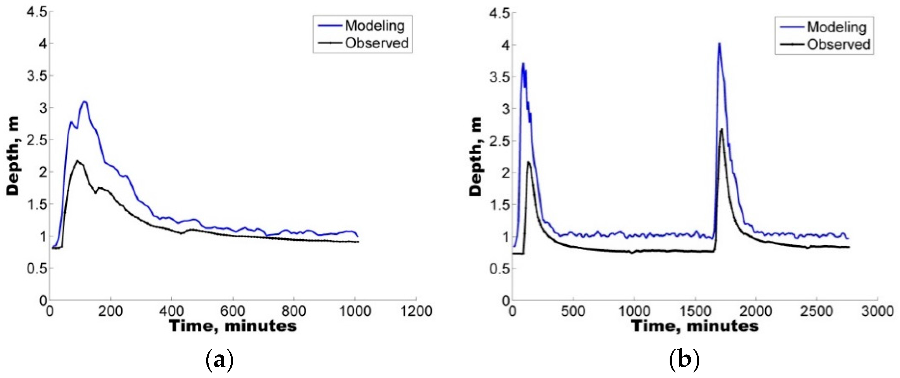
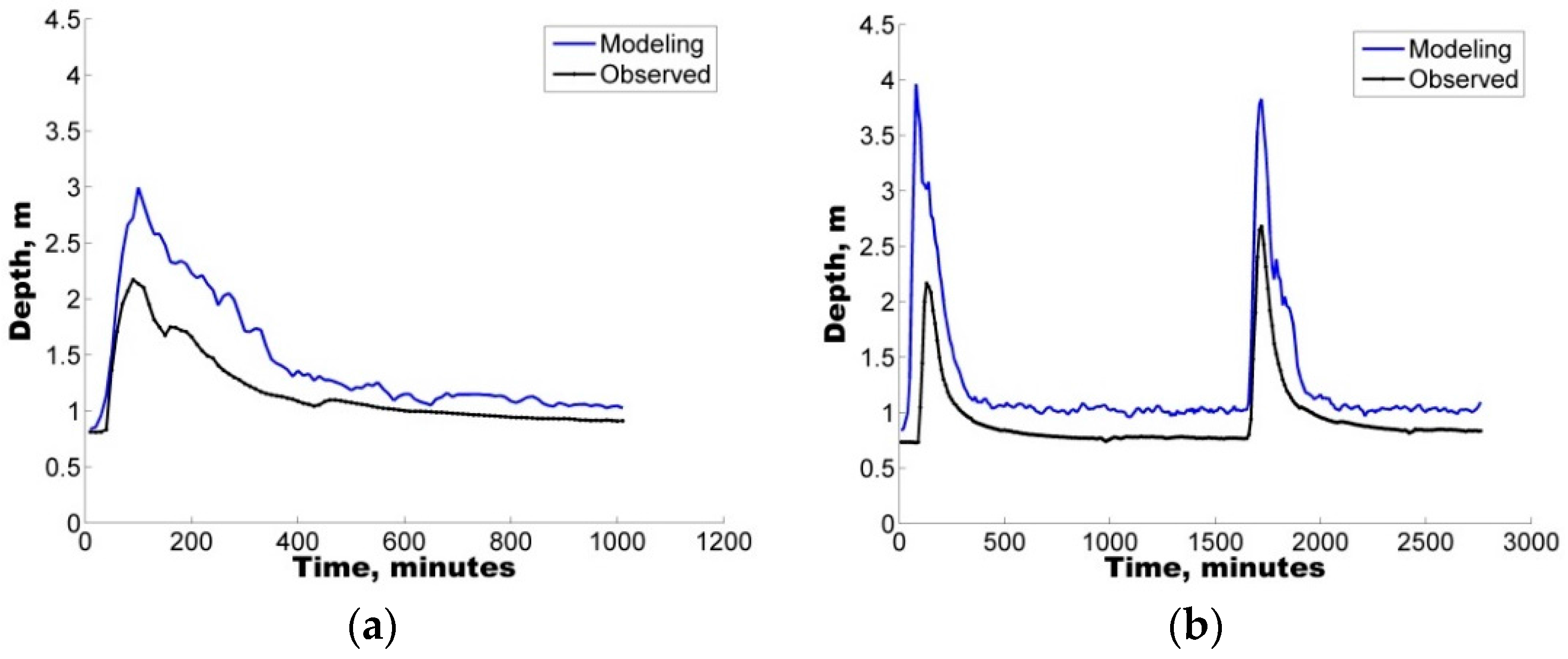
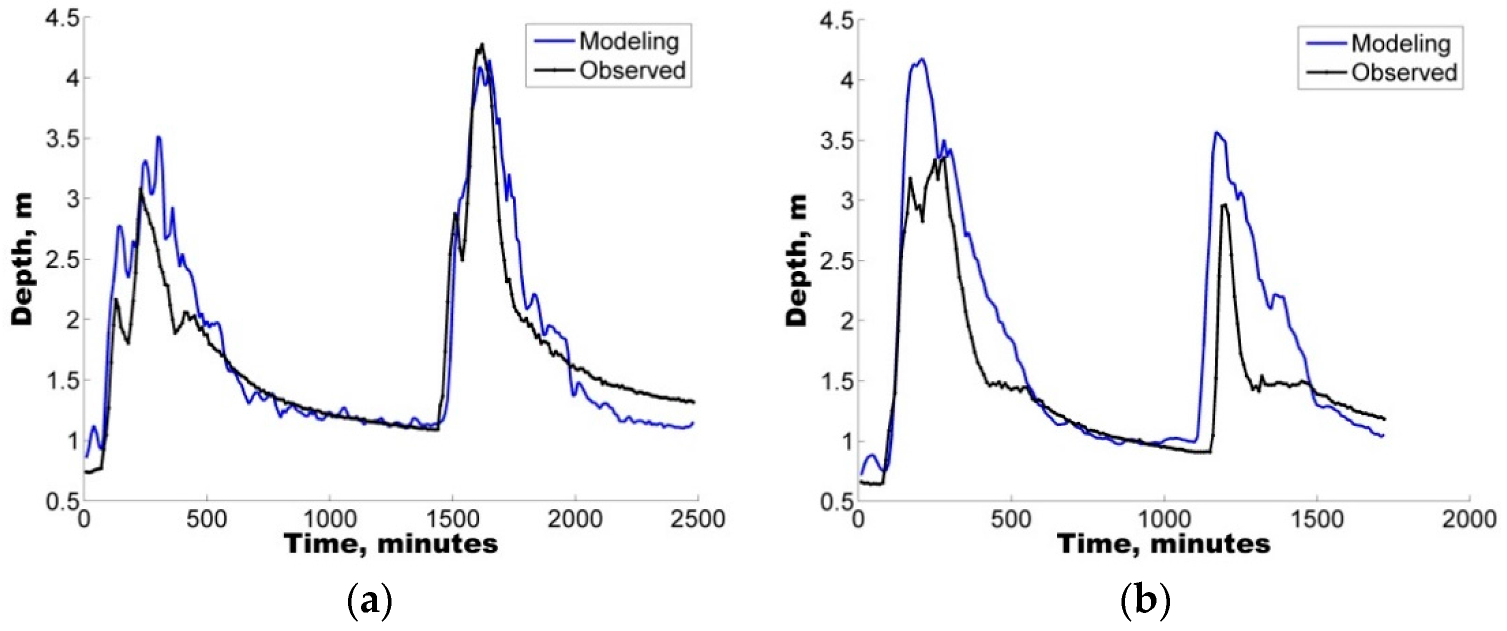
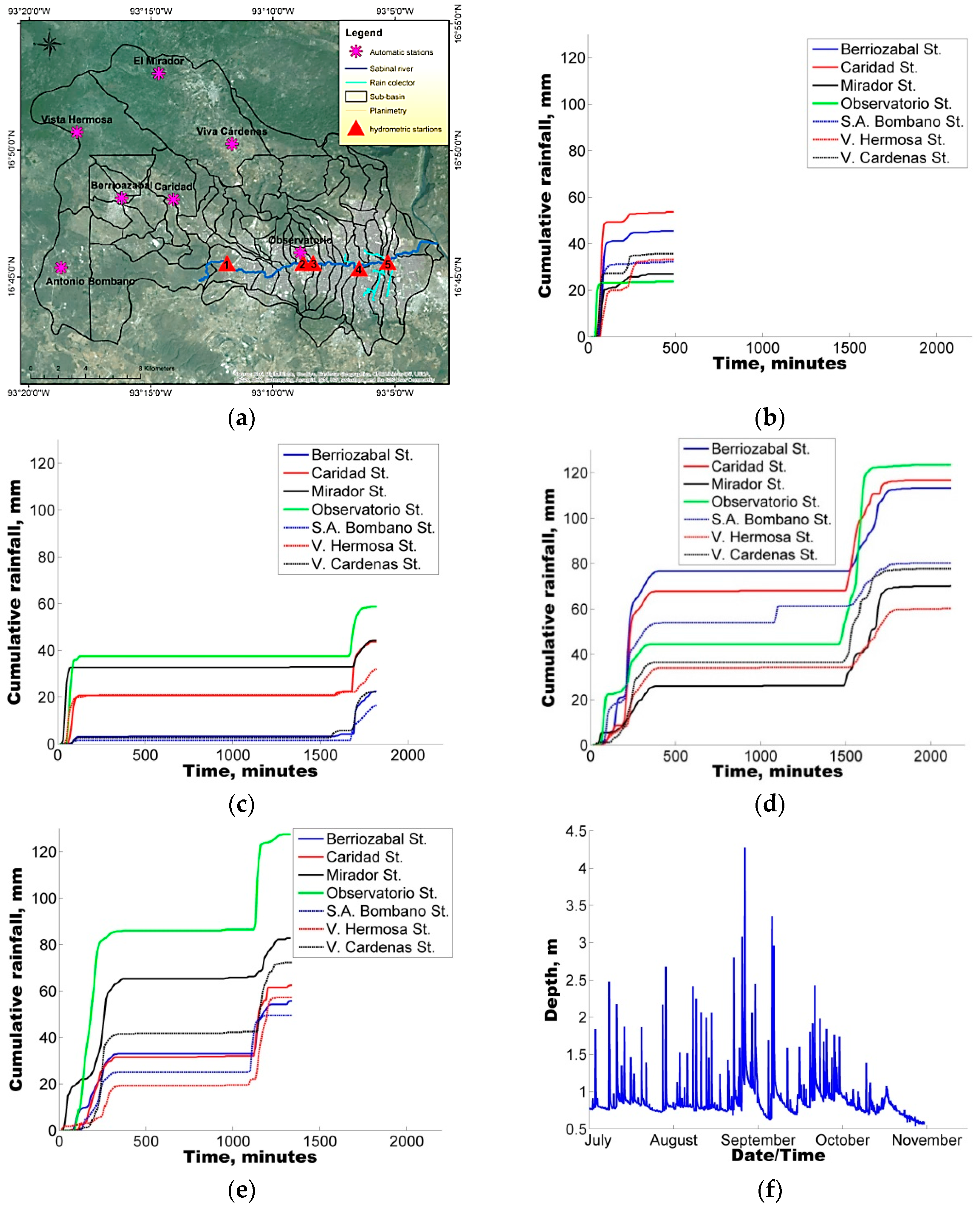
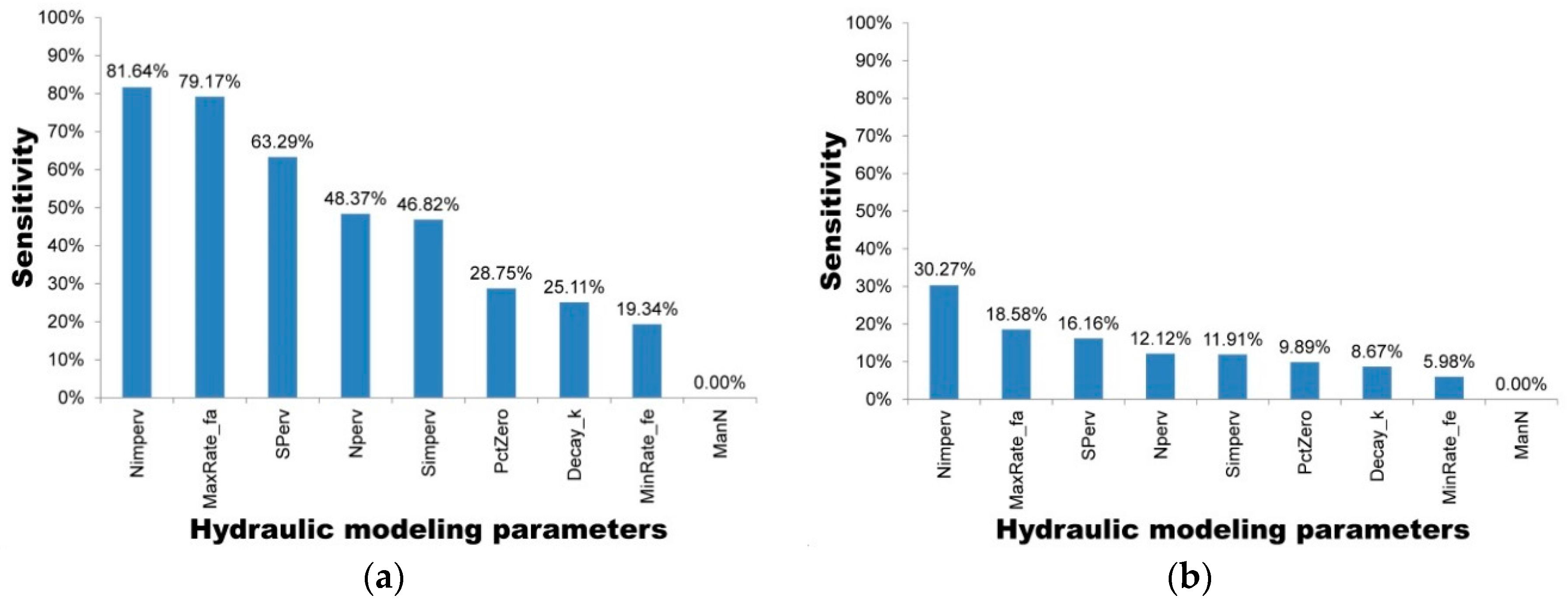
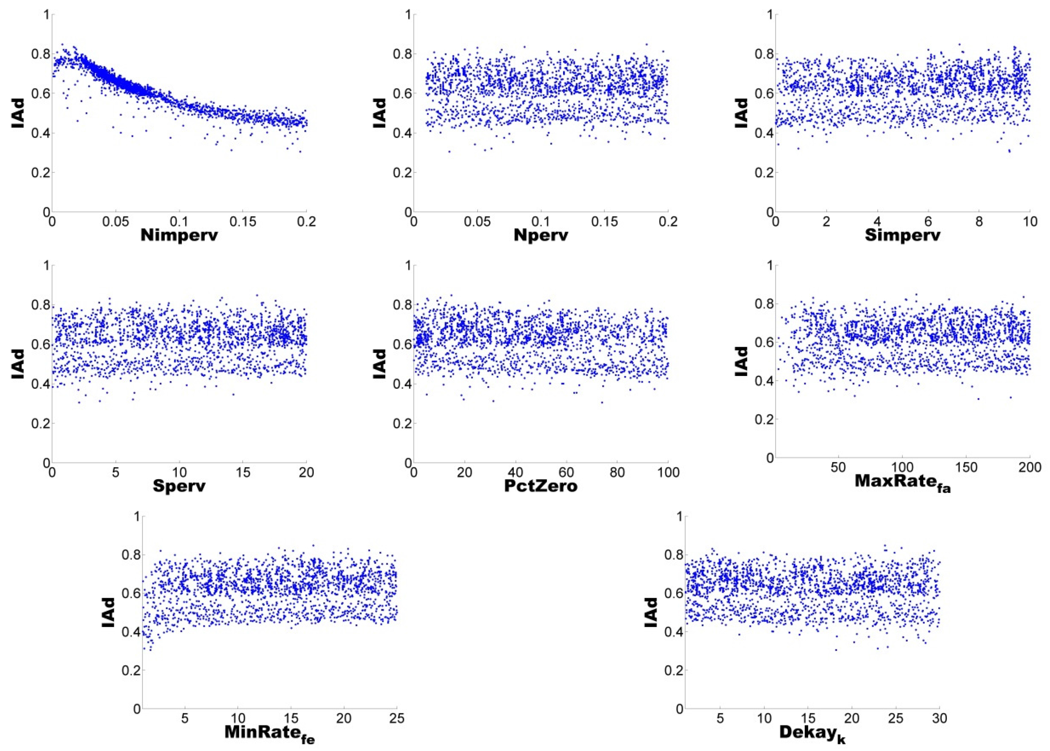
The model was first implemented in the study area followed by a sensitivity analysis of eight selected parameters. To identify the sets of parameters that allowed for a good representation of the rainfall-runoff response, four rainfall events varying from 20.0 mm to 120.2 mm were selected to ensure the applicability and reliability of the model for varying conditions from minor to major events.

Additionally, with the purpose of quantifying the uncertainty ascribed to the definition of parameters in the hydrological model, two different uncertainty analysis techniques were also implemented, GLUE and AMALGAM. For the four selected storms, both techniques were found to generate results with similar skill (ARIL), both generating parameter sets with IAd greater than 60%, i.e., good model performance.

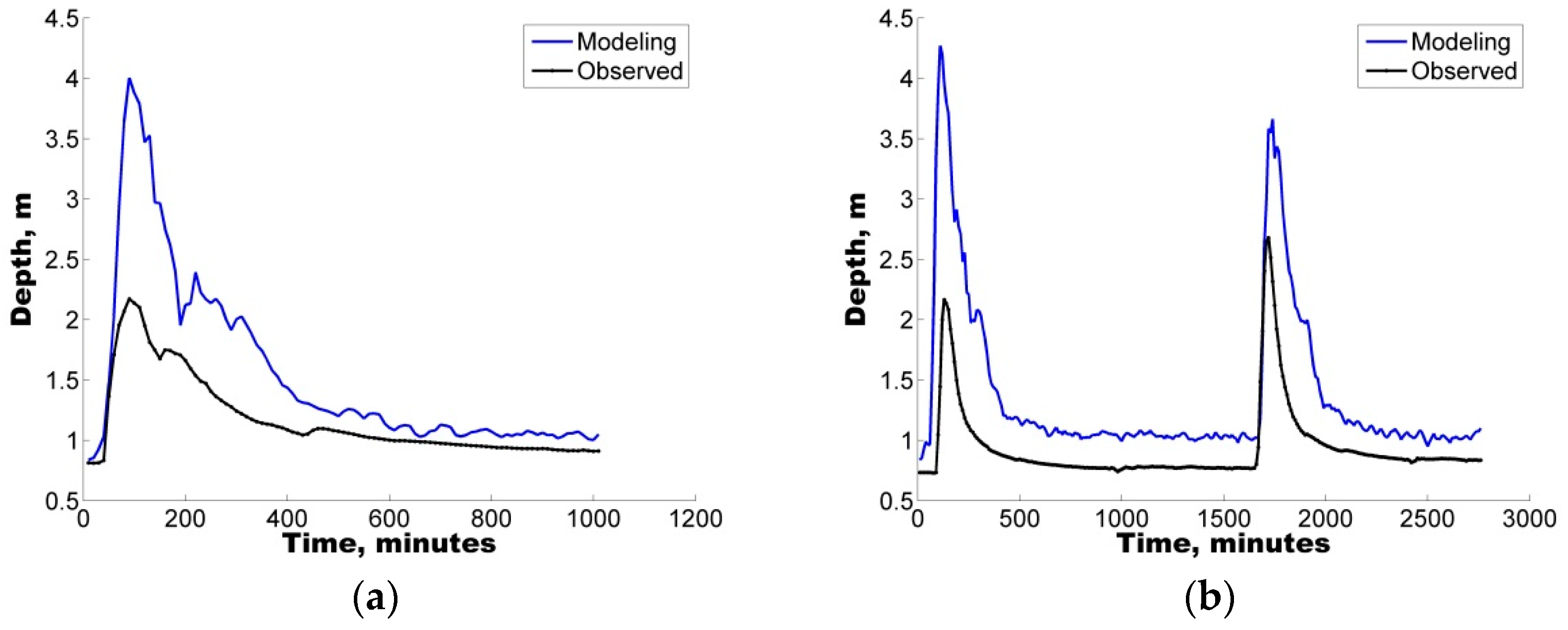
In all cases, the results show that hydrological predictions are more reliable when model deficiencies (e.g., parameter uncertainty) are considered. In addition to the use of the IAd, to complement the analysis, the APE values were used to select the optimal parameter sets for the calibration/validation of the study case.

Notably, an average EAP lower than 30% was observed in some of the depth sets, considering the parameter sets obtained from the uncertainty analysis. Therefore, the quantification of different error contributions enables the generation of more reliable flow predictions.

This investigation clearly shows the advantages of implementing a sensitivity analysis and uncertainty approach when modelling the rainfall-runoff response in data scarce countries. The selected approach seems to be promising with regards to the identification of the posterior parameter distributions and also elucidates the aggregation of errors within a modelling framework, suggesting the importance of parameter interaction.

Note that, in cases where data scarcity is high, the implementation of methods that enable the quantification of uncertainty in model predictions enables more transparent results that show the effects of aggregation of errors arising from different sources within a prediction. Both implemented techniques showed that there are several parameter sets that provide a good representation of the system. The ability to have an uncertainty band associated with the model predictions minimises the subjectivity associated with the predictions. Further work should be performed to investigate the impact of the initial parameter distribution on the posterior distribution generated with a Monte-Carlo procedure, particularly in cases where highly correlated parameters are present.

References

1. Cashion, J.; Lakshmi, V.; Bosch, D.; Jackson, T.J. Microwave remote sensing of soil moisture: Evaluation of the TRMM microwave imager (TMI) satellite for the Little River Watershed Tifton, Georgia. J. Hydrol. 2005, 307, 242–253. [Google Scholar] [CrossRef]
2. Sorooshian, A.; Wonaschütz, A.; Jarjour, E.G.; Hashimoto, B.I.; Schichtel, B.A.; Betterton, E.A. An aerosol climatology for a rapidly growing arid region (southern Arizona): Major aerosol species and remotely sensed aerosol properties. J. Geophys. Res. Atmos. 2011, 116. [Google Scholar] [CrossRef] [PubMed]
3. Sellars, S.; Nguyen, P.; Chu, W.; Gao, X.; Hsu, K.; Sorooshian, S. Computational Earth Science: Big Data Transformed Into Insight. EOS Trans. Am. Geophys. Union 2013, 94, 277–278. [Google Scholar] [CrossRef]
4. Hamel, P.; Fletcher, T.D. Modelling the impact of stormwater source control infiltration techniques on catchment baseflow. Hydrol. Process. 2014, 28, 5817–5831. [Google Scholar] [CrossRef]
5. Petrucci, G.; Bonhomme, C. The dilemma of spatial representation for urban hydrology semi-distributed modelling: Trade-offs among complexity, calibration and geographical data. J. Hydrol. 2014, 517, 997–1007. [Google Scholar] [CrossRef]
6. Vrebos, D.; Vansteenkiste, T.; Staes, J.; Willems, P.; Meire, P. Water displacement by sewer infrastructure in the Grote Nete catchment, Belgium, and its hydrological regime effects. Hydrol. Earth Syst. Sci. 2014, 18, 1119–1136. [Google Scholar] [CrossRef] [Green Version]
7. McMillan, H.; Jackson, B.; Clark, M.; Kavetski, D.; Woods, R. Rainfall uncertainty in hydrological modelling: An evaluation of multiplicative error models. J. Hydrol. 2011, 400, 83–94. [Google Scholar] [CrossRef]
8. Hughes, D.A. A review of 40 years of hydrological science and practice in southern Africa using the Pitman rainfall-runoff model. J. Hydrol. 2013, 501, 111–124. [Google Scholar] [CrossRef]
9. Montanari, A.; Koutsoyiannis, D. A blueprint for process-based modeling of uncertain hydrological systems. Water Resour. Res. 2012, 48, W09555. [Google Scholar] [CrossRef]
10. Rodriguez-Rincon, J.P.; Pedrozo-Acuña, A.; Breña-Naranjo, J.A. Propagation of hydro-meteorological uncertainty in a model cascade framework to inundation prediction. Hydrol. Earth Syst. Sci. 2015, 19, 2981–2998. [Google Scholar] [CrossRef]
11. Beven, K.; Binley, A. The future of distributed Models: Model Calibration and Uncertainty Prediction. Hydrol. Process. 1992, 6, 279–298. [Google Scholar] [CrossRef]
12. Beven, K.; Westerberg, I. On red herrings and real herrings: Disinformation and information in hydrological inference. Hydrol. Process. 2011, 25, 1676–1680. [Google Scholar] [CrossRef]
13. McMillan, H.; Krueger, T.; Freer, J. Benchmarking observational uncertainties for hydrology: Rainfall, river discharge and water quality. Hydrol. Process. 2012, 26, 4078–4111. [Google Scholar] [CrossRef]
14. Razavi, T.; Coulibaly, P. Streamflow Prediction in Ungauged Basins: Review of Regionalization Methods. J. Hydrol. Eng. 2013, 18, 958–975. [Google Scholar] [CrossRef]
15. Refsgaard, J.C.; van der Sluijs, J.P.; Brown, J.; van der Keur, P. A framework for dealing with uncertainty due to model structure error. Adv. Water Resour. 2006, 29, 1586–1597. [Google Scholar] [CrossRef]
16. Crespo, P.J.; Feyen, J.; Buytaert, W.; Bücker, A.; Breuer, L.; Frede, H.G.; Ramírez, M. Identifying controls of the rainfall–runoff response of small catchments in the tropical Andes. J. Hydrol. 2011, 407, 164–174. [Google Scholar] [CrossRef]
17. Kuczera, G.; Renard, B.; Thyer, M.; Kavetski, D. There are no hydrological monsters, just models and observations with large uncertainties. Hydrol. Sci. J. 2010, 55, 980–991. [Google Scholar] [CrossRef]
18. Van Griensven, A.; Meixner, T. Dealing with unidentifiable sources of uncertainty within environmental models. In Proceedings of the International Environmental Modelling and Software Society, University of Osnabrück, Osnabrück, Germany, 14–17 June 2004.
19. Beven, K.; Freer, J. Equifinality, data assimilation, and uncertainty estimation in mechanistic modelling of complex environmental systems using the GLUE methodology. J. Hydrol. 2001, 249, 11–29. [Google Scholar] [CrossRef]
20. Peel, M.C.; Blöschl, G. Hydrological modelling in a changing world. Prog. Phys. Geogr. 2011, 35, 249–261. [Google Scholar] [CrossRef]
21. Wagener, T.; Kollat, J. Numerical and visual evaluation of hydrological and environmental models using the Monte Carlo analysis toolbox. Environ. Model. Softw. 2007, 22, 1021–1033. [Google Scholar] [CrossRef]
22. Wagener, T.; Gupta, H.V. Model identification for hydrological forecasting under uncertainty. Stoch. Environ. Res. Risk Assess. 2005, 19, 378–387. [Google Scholar] [CrossRef]
23. Dotto, C.; Kleidorfer, M.; Deletic, A.; Rauch, W.; McCarthy, D.; Fletcher, T. Performance and sensitivity analysis of stormwater models using a Bayesian approach and long-term high resolution data. Environ. Model. Softw. 2011, 26, 1225–1239. [Google Scholar] [CrossRef]
24. Dotto, C.B.; Kleidorfer, M.; Deletic, A.; McCarthy, D.T.; Rauch, W. Stormwater quality models: Performance and sensitivity analysis. Water Sci. Technol. 2010, 62, 837–843. [Google Scholar] [CrossRef] [PubMed]
25. Freni, G.; Mannina, G.; Viviani, G. Urban runoff modelling uncertainty: Comparison among Bayesian and pseudo-Bayesian methods. Environ. Model. Softw. 2009, 24, 1100–1111. [Google Scholar] [CrossRef]
26. Vrugt, J.A.; Gupta, H.V.; Bouten, W.; Sorooshian, S. A Shuffled Complex Evolution Metropolis algorithm for optimization and uncertainty assessment of hydrologic model parameters. Water Resour. Res. 2003, 39. [Google Scholar] [CrossRef]
27. Vrugt, J.A.; Gupta, H.V.; Bastidas, L.A.; Bouten, W.; Sorooshian, A. Effective and efficient algorithm for multiobjective optimization of hydrologic models. Water Resour. Res. 2003, 39. [Google Scholar] [CrossRef]
28. Vrugt, J.A.; Braak, C.T.; Diks, C.; Robinson, B.A.; Hyman, J.M.; Higdon, D. Accelerating Markov Chain Monte Carlo Simulation by Differential Evolution with Self-Adaptive Randomized Subspace Sampling. Int. J. Nonlinear Sci. Numer. Simul. 2009, 10, 271–288. [Google Scholar] [CrossRef]
29. Beven, K.; Freer, J.; Hankin, B.; Schulz, K. The Use of Generalised Likelihood Measures for Uncertainty Estimation in High Order Models of Environmental Systems. In Nonlinear and Nonstationary Signal Processing; Fitzgerald, W.J., Smith, R.L., Waldon, A.T., Young, P.C., Eds.; Cambridge University Press: New York, NY, USA, 2000; pp. 115–151. [Google Scholar]
30. Knighton, J.; Lennon, E.; Bastidas, L.; White, E. Stormwater detention system parameter sensitivity and uncertainty analysis using SWMM. J. Hydrol. Eng. 2016, 21, 05016014. [Google Scholar] [CrossRef]
31. Fraga, I.; Cea, L.; Puertas, J.; Suárez, J.; Jiménez, V.; Jácome, A. Global sensitivity and GLUE-based uncertainty analysis of a 2D-1D dual urban drainage model. J. Hydrol. Eng. 2016, 21, 04016004. [Google Scholar] [CrossRef]
32. Sun, N.; Hall, M.; Hong, B.; Zhang, L.J. Impact of SWMM catchment discretization: Case study in Syracuse, New York. J. Hydrol. Eng. 2014, 19, 223–234. [Google Scholar] [CrossRef]
33. Zhao, D.; Chen, J.; Wang, H.; Tong, Q. Application of a sampling based on the combined objectives of parameter identification and uncertainty analysis of an urban rainfall-runoff model. J. Irrig. Drain. Eng. 2013, 139, 66–74. [Google Scholar] [CrossRef]
34. Sivapalan, M. Prediction in ungauged basins: A grand challenge for theoretical hydrology. Hydrol. Process. 2003, 17, 3163–3170. [Google Scholar] [CrossRef]
35. Sivapalan, M.; Takeuchi, K.; Franks, S.W.; Gupta, V.K.; Karambiri, H.; Lakshmi, V.; Liang, X.; McDonnell, J.J.; Mendiondo, E.M.; O’Connell, P.E.; et al. IAHS Decade on Predictions in Ungauged Basins (PUB), 2003–2012: Shaping an exciting future for the hydrological sciences. Hydrol. Sci. J. 2003, 48, 857–880. [Google Scholar] [CrossRef]
36. Vrugt, J.A.; Robinson, B.A. Improved evolutionary optimization from genetically adaptive multimethod search. Proc. Natl. Acad. Sci. USA 2007, 104, 708–711. [Google Scholar] [CrossRef] [PubMed]
37. Dotto, C.B.; Mannina, G.; Kleidorfer, M.; Vezzaro, L.; Henrichs, M.; McCarthy, D.T.; Freni, G.; Rauch, W.; Deletic, A. Comparison of different uncertainty techniques in urban stormwater quantity and quality modelling. Water Res. 2012, 46, 2545–2558. [Google Scholar] [CrossRef] [PubMed]
38. Jin, X.; Xu, C.Y.; Zhang, Q.; Singh, V. Parameter and modeling uncertainty simulated by GLUE and a formal Bayesian method for a conceptual hydrological model. J. Hydrol. 2010, 383, 147–155. [Google Scholar] [CrossRef]
39. Li, L.; Xia, J.; Xu, C.Y.; Singh, V. Evaluation of the subjective factors of the GLUE method and comparison with the formal Bayesian method in uncertainty assessment of hydrological models. J. Hydrol. 2010, 390, 210–221. [Google Scholar] [CrossRef]
40. Yang, J.; Reichert, P.; Abbaspour, K.; Xia, J.; Yang, H. Comparing uncertainty analysis techniques for a SWAT application to the Chaohe Basin in China. J. Hydrol. 2008, 358, 1–23. [Google Scholar] [CrossRef]
41. Willmot, C.J. On the validation of models. Phys. Geogr. 1981, 2, 184–194. [Google Scholar]
42. Krause, P.; Boyle, D.P.; Bäse, F. Comparison of different efficiency criteria for hydrological model assessment. Adv. Geosci. 2005, 5, 89–97. [Google Scholar] [CrossRef]
43. James, W.; Rossman, L.E.; James, W.R.C. User’s Guide to SWMM5, 13th ed.; CHI: Guelph, ON, Canada, 2010. [Google Scholar]
44. Uhl, M.; Henrichs, M. Kalibrierung von hydrologischen Prozessmodellen, Programm-Dokumentation, Version 3.0; IWARU: Münster, Germany, 2014. [Google Scholar]
45. Mannina, G.; Viviano, G. An urban drainage stormwater quality model: Model development and uncertainty quantification. J. Hydrol. 2010, 381, 248–265. [Google Scholar] [CrossRef]
46. Mantovan, P.; Todini, E. Hydrological forecasting uncertainty assessment: Incoherence of the GLUE methodology. J. Hydrol. 2006, 330, 368–381. [Google Scholar] [CrossRef]
47. Freni, G.; Mannina, G.; Viviani, G. Uncertainty in urban stormwater quality modelling: The influence of likelihood measure formulation in the GLUE methodology. Sci. Total Environ. 2009, 408, 138–145. [Google Scholar] [CrossRef] [PubMed]
48. Huisman, J.A.; Rings, J.; Vrugt, J.A.; Sorg, J.; Vereecken, H. Hydraulic properties of a model dike from coupled Bayesian and multi-criteria hydrogeophysical inversion. J. Hydrol. 2010, 380, 62–73. [Google Scholar] [CrossRef]
49. Deb, K.; Pratap, A.; Agarwal, S.; Meyarivan, T. A fast and elitist Multiobjective Genetic Algorithm: NSGA-II. IEEE Trans. Evol. Comput. 2002, 6, 182–197. [Google Scholar] [CrossRef]
50. Kennedy, J.; Eberhart, R.C.; Shi, Y. Swarm Intelligence; Morgan Kaufmann: San Francisco, CA, USA, 2001. [Google Scholar]
51. Haario, H.; Saksman, E.; Tamminen, J. An adaptive Metropolis algorithm. Bernoulli 2001, 7, 223–242. [Google Scholar] [CrossRef]
52. Storn, R.; Price, K. Differential Evolution—A Simple and Efficient Heuristic for Global Optimization over Continuous Spaces. J. Glob. Optim. 1997, 11, 341–359. [Google Scholar] [CrossRef]
53. Butts, M.B.; Payne, J.T.; Kristensen, M.; Madsen, H. An evaluation of the impact of model structure on hydrological modelling uncertainty for streamflow simulation. J. Hydrol. 2004, 298, 242–266. [Google Scholar] [CrossRef]
54. Wan, B.; James, W. SWMM Calibration using genetic algorithms. J. Water Manag. Model. 2002. [Google Scholar] [CrossRef]
55. Knight, D.W.; Shamseldin, A.Y. Quantitative precipitation forecasting. In River Basin Modelling for Flood Risk Mitigation, 1st ed.; Taylor & Francis/Balkema: Leiden, The Netherlands, 2006; pp. 146–150. [Google Scholar]
56. James, W. Rules for Responsible Modeling, 4th ed.; CHI: Guelph, ON, Canada, 2005; pp. 211–213. [Google Scholar]
Figure 1. Uncertainty analysis methodology.
Water 08 00524 g001
Figure 2. (a) Urban basin of Tuxtla Gutierrez, Mexico; Rainfall events; (b) Event 1; (c) Event 2; (d) Event 3; and (e) Event 4; and (f) Hydrometric station 5 from 1 July 2011 to 31 October 2011.
Water 08 00524 g002
Figure 3. Generated depth via the observed precipitation and initial hydrologic parameters compared with the observed depth: (a) Event 1 and (b) Event 2.
Water 08 00524 g003
Figure 4. Sensitivity of the model parameters of urban drainage: (a) maximum sensitivity and (b) average sensitivity.
Water 08 00524 g004
Figure 5. Distribution of 2000 sets of parameters, method GLUE, Event 1.
Water 08 00524 g005
Figure 6. Distribution of 2000 sets of parameters, AMALGAM method, Event 1.
Water 08 00524 g006
Figure 7. Confidence band of 95%, GLUE technique: (a) Event 1 and (b) Event 2.
Water 08 00524 g007
Figure 8. Confidence band of 95%, AMALGAM technique: (a) Event 1 and (b) Event 2.
Water 08 00524 g008
Figure 9. Depth levels of Sabinal River for (a) Event 1 & C276 and (b) Event 2 & C272, using parameter sets obtained by GLUE.
Water 08 00524 g009
Figure 10. Depth levels of Sabinal River for (a) Event 1 & C365 and (b) Event 2 & C1501, using parameter sets obtained by AMALGAM.
Water 08 00524 g010
Figure 11. Validation of the depth levels of the Sabinal River using the optimal parameter set, C365, obtained by the method AMALGAM for (a) Event 3 and (b) Event 4.
Water 08 00524 g011
Figure 12. Validation of the depth levels of the Sabinal River using non-uniform distribution of Nimperv parameter, for (a) Event 1 and (b) Event 2.
Water 08 00524 g012
Figure 13. Validation of the depth levels of the Sabinal River using non-uniform distribution of Nimperv parameter, for (a) Event 3 and (b) Event 4.
Water 08 00524 g013