
Using GOCI Retrieval Data to Initialize and Validate a Sediment Transport Model for Monitoring Diurnal Variation of SSC in Hangzhou Bay, China


Abstract
:1. Introduction
2. Data and Methods
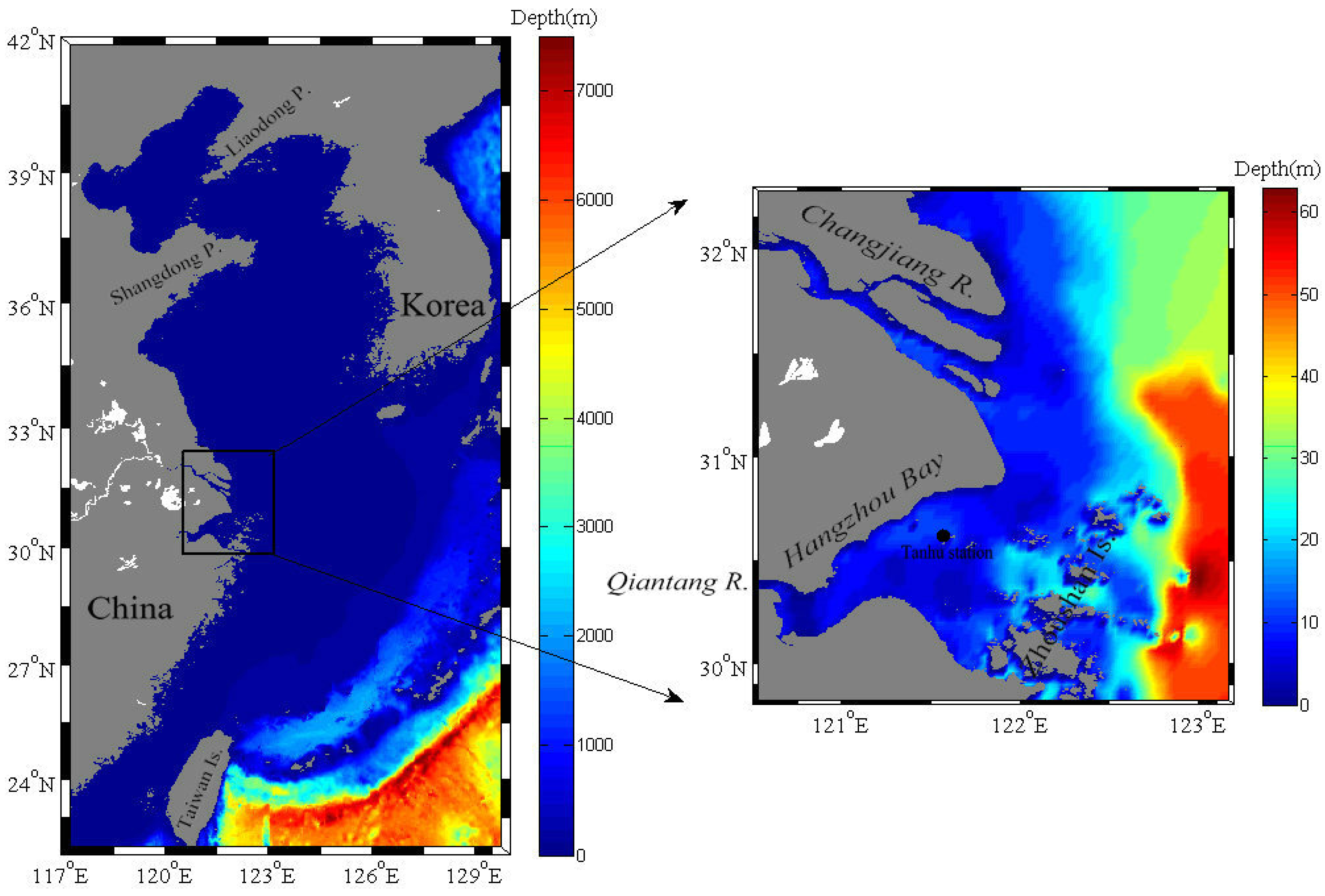
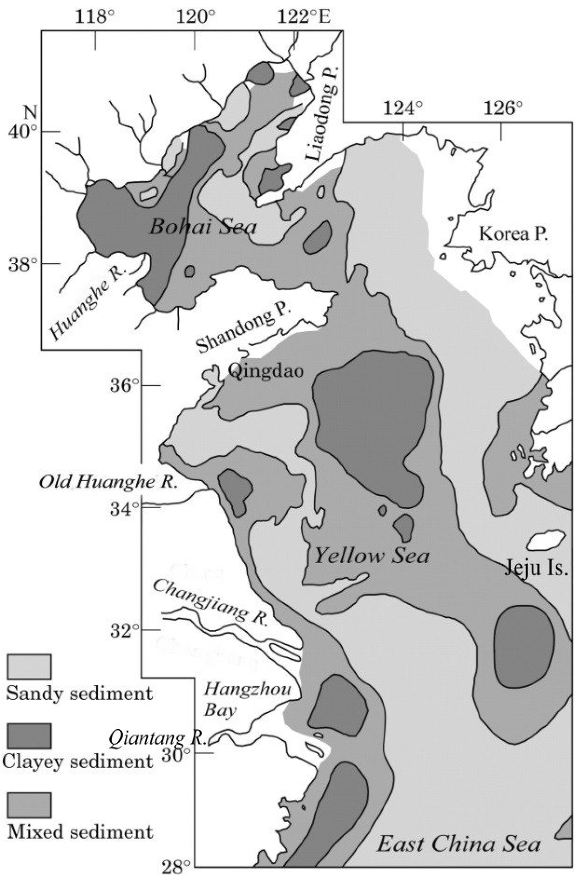
2.1. Study Area
2.2. Retrieval of SSC from GOCI
2.3. Sediment Transport Modeling
2.3.1. Hydrodynamic Module Configuration
2.3.2. Sediment Module Configuration
3. Results and Discussion
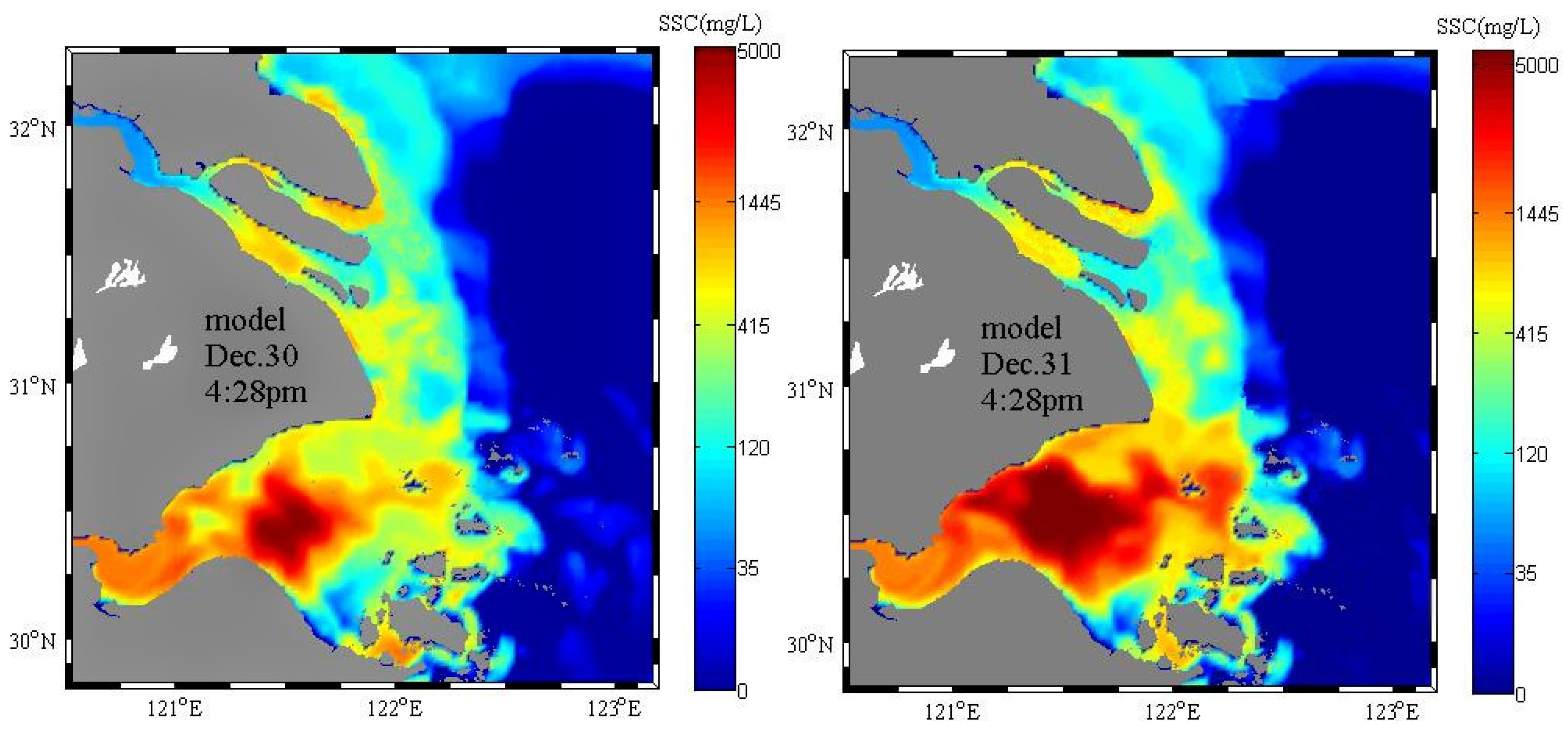
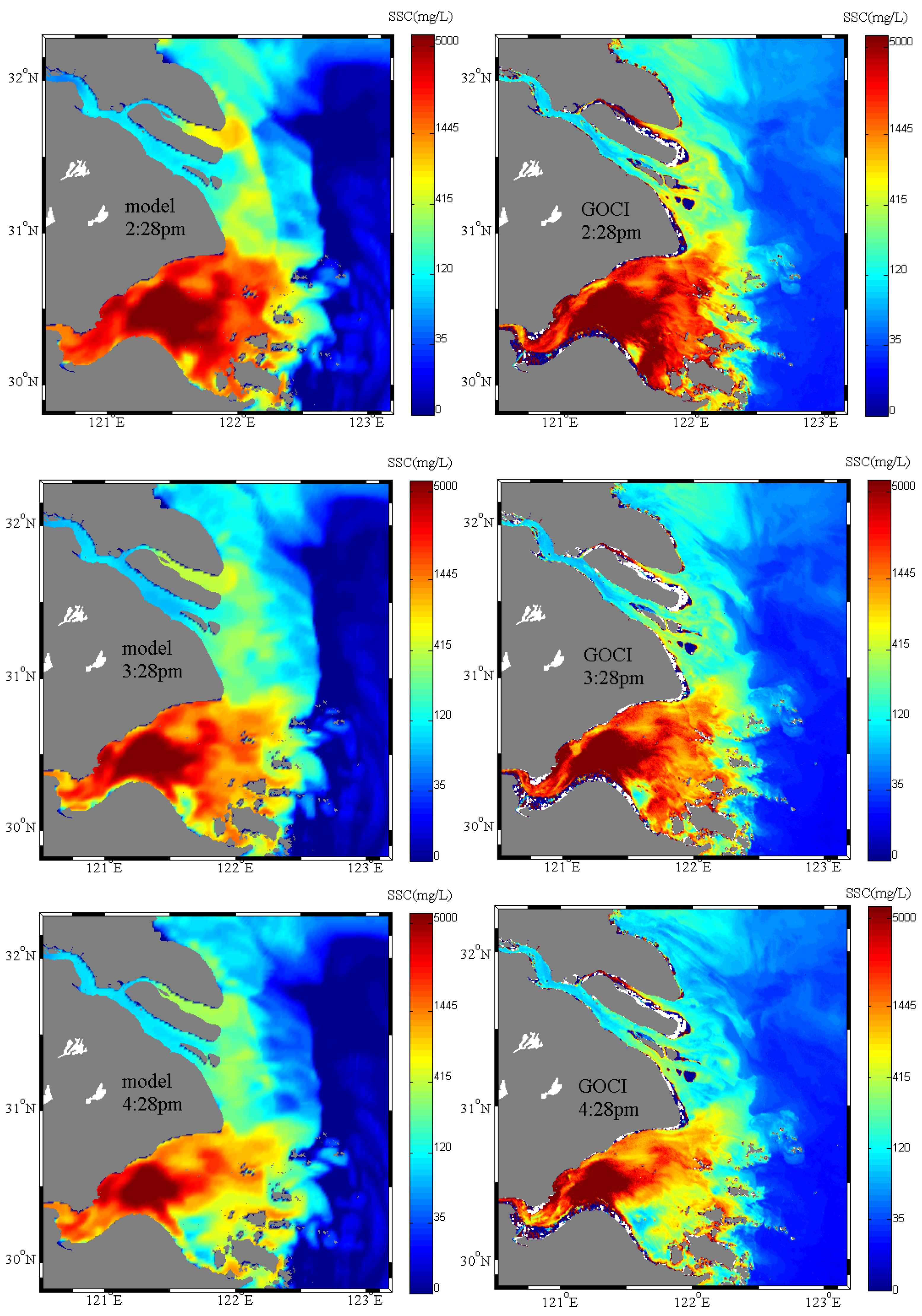
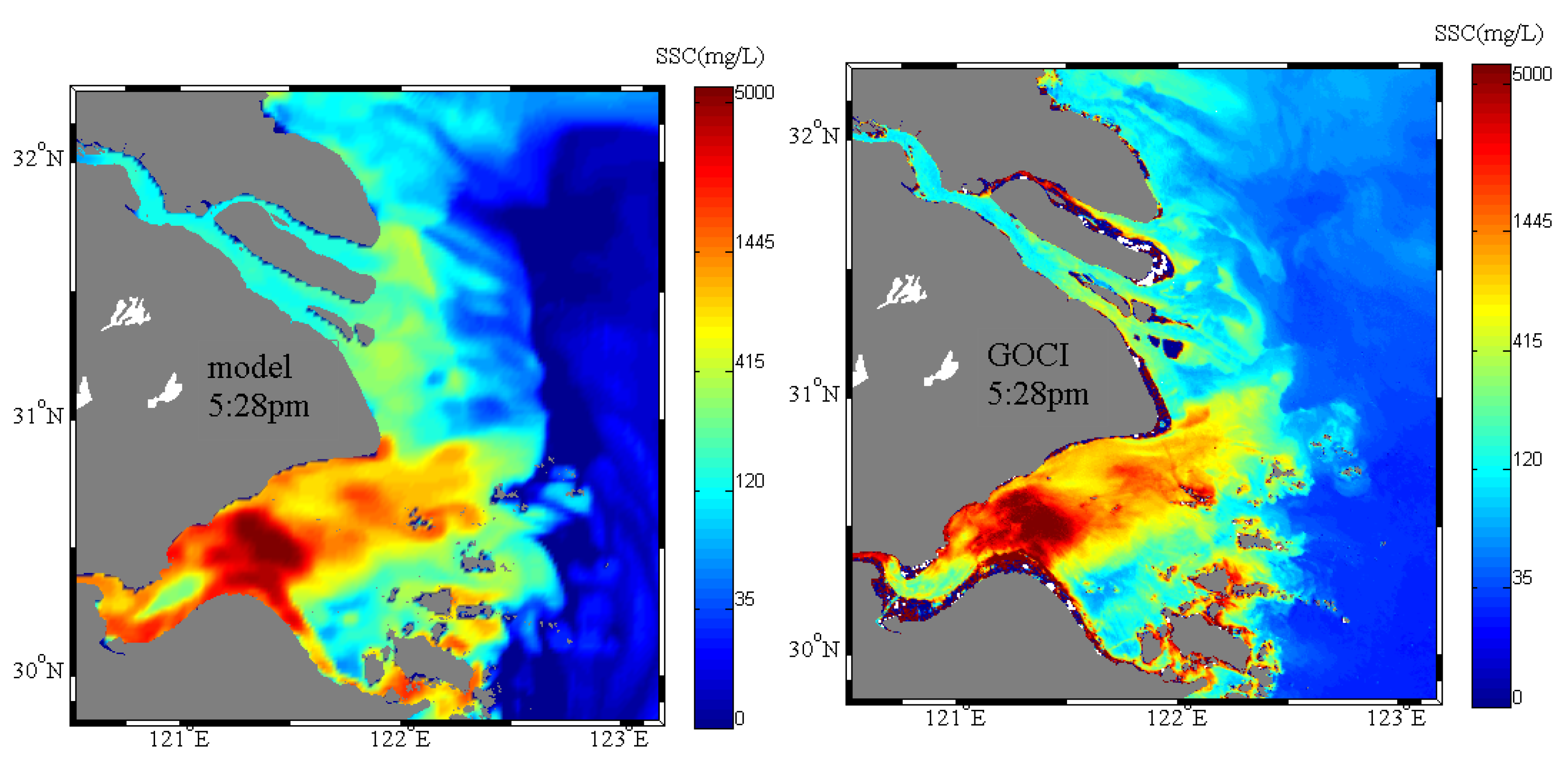
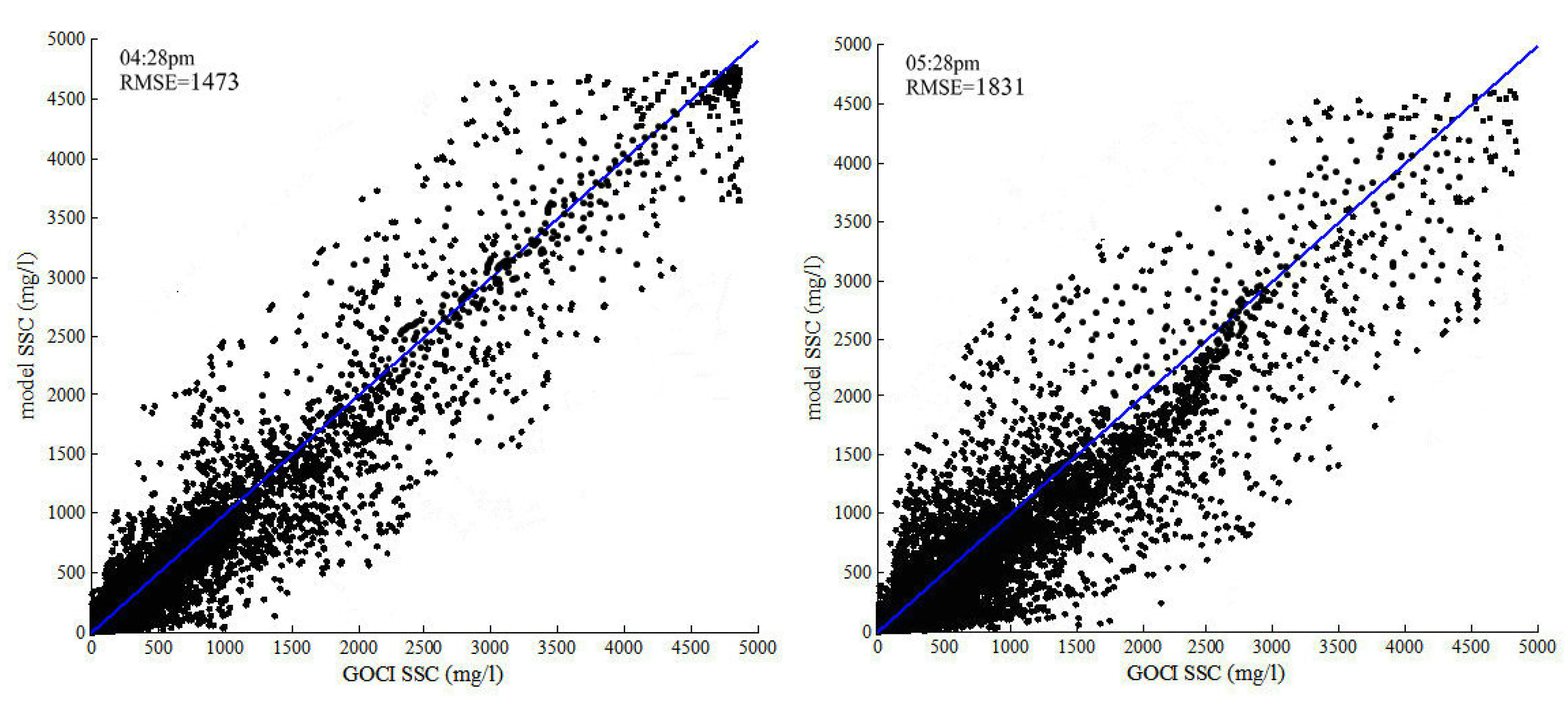
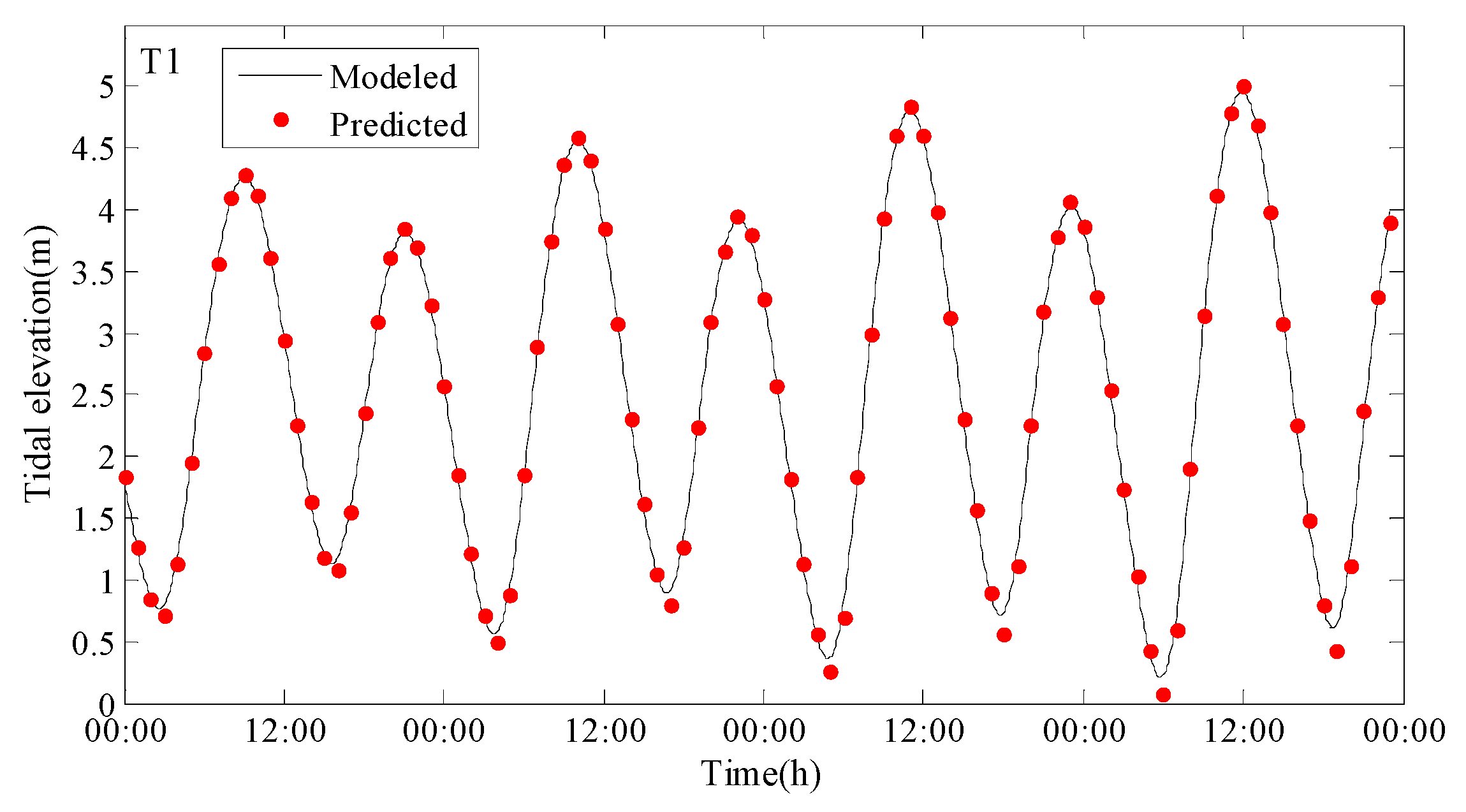
3.1. Sediment Model Initialization and Validation
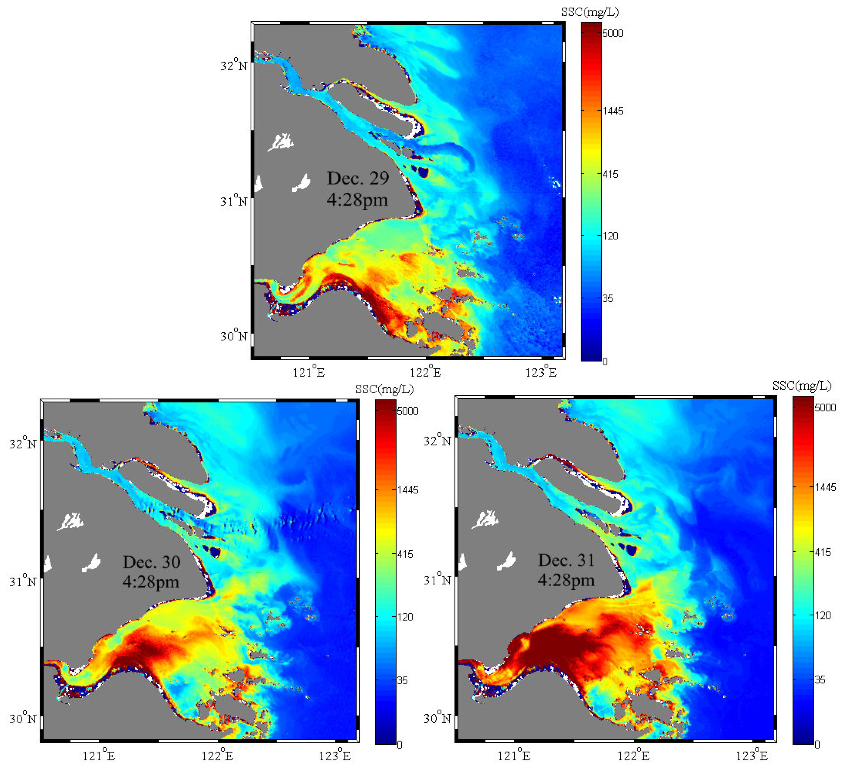
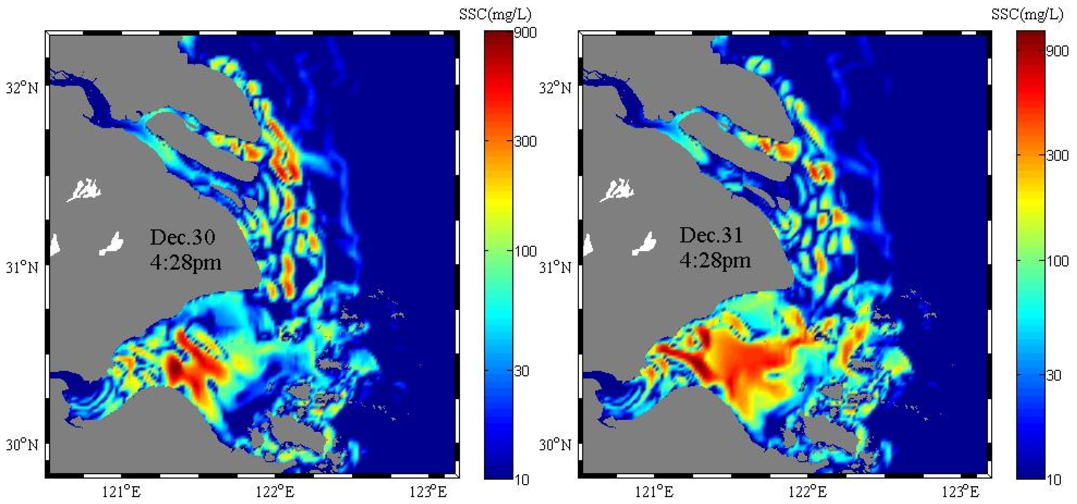
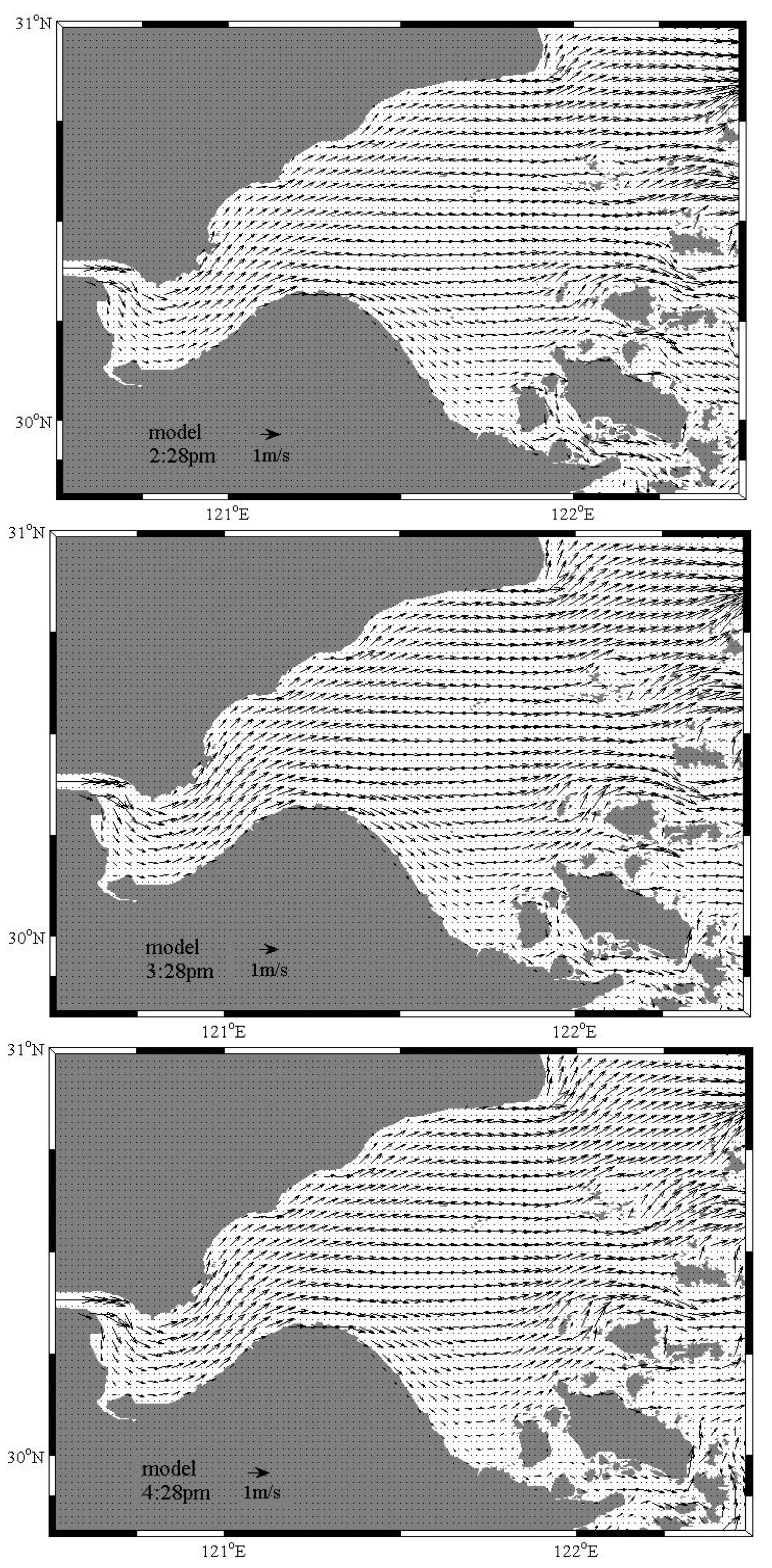
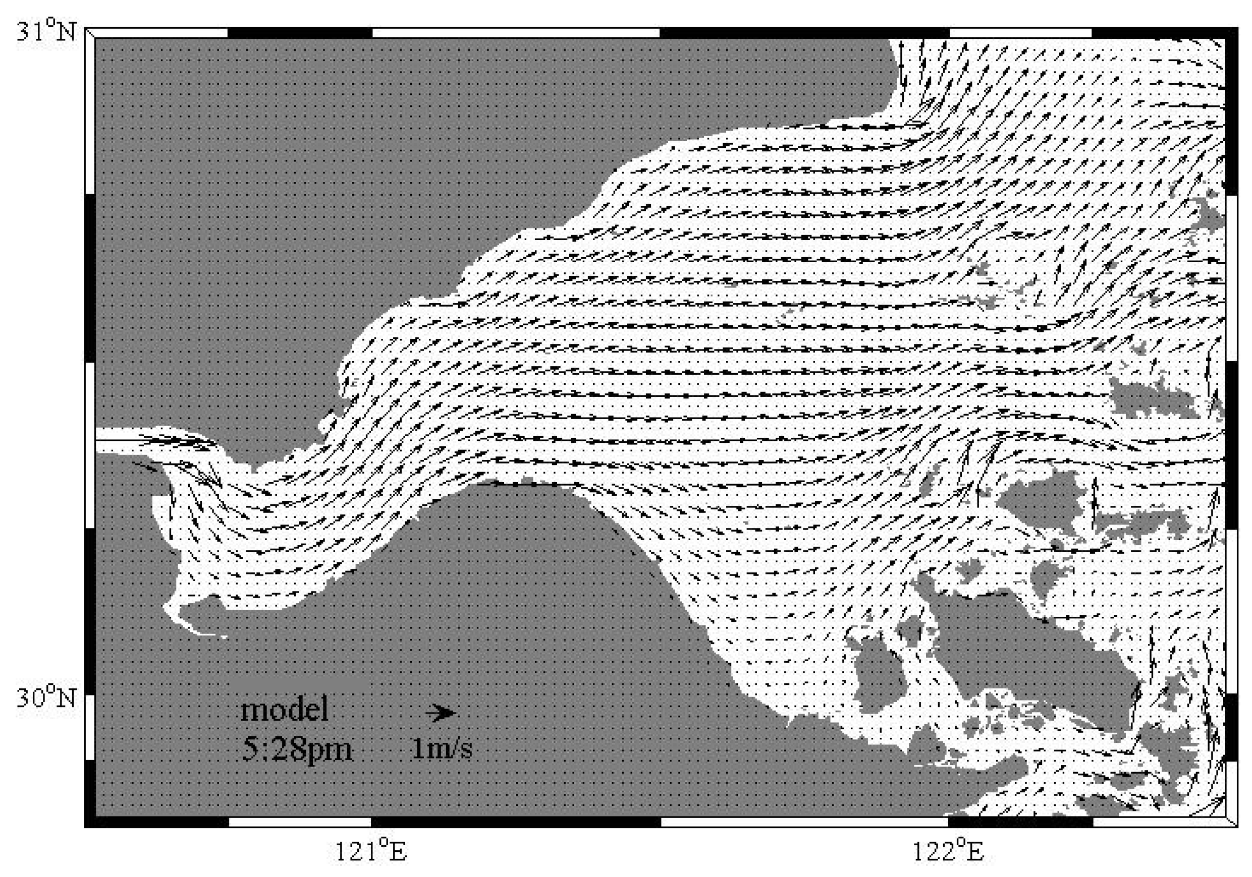
3.2. The Diurnal Variation of Suspended Sediment
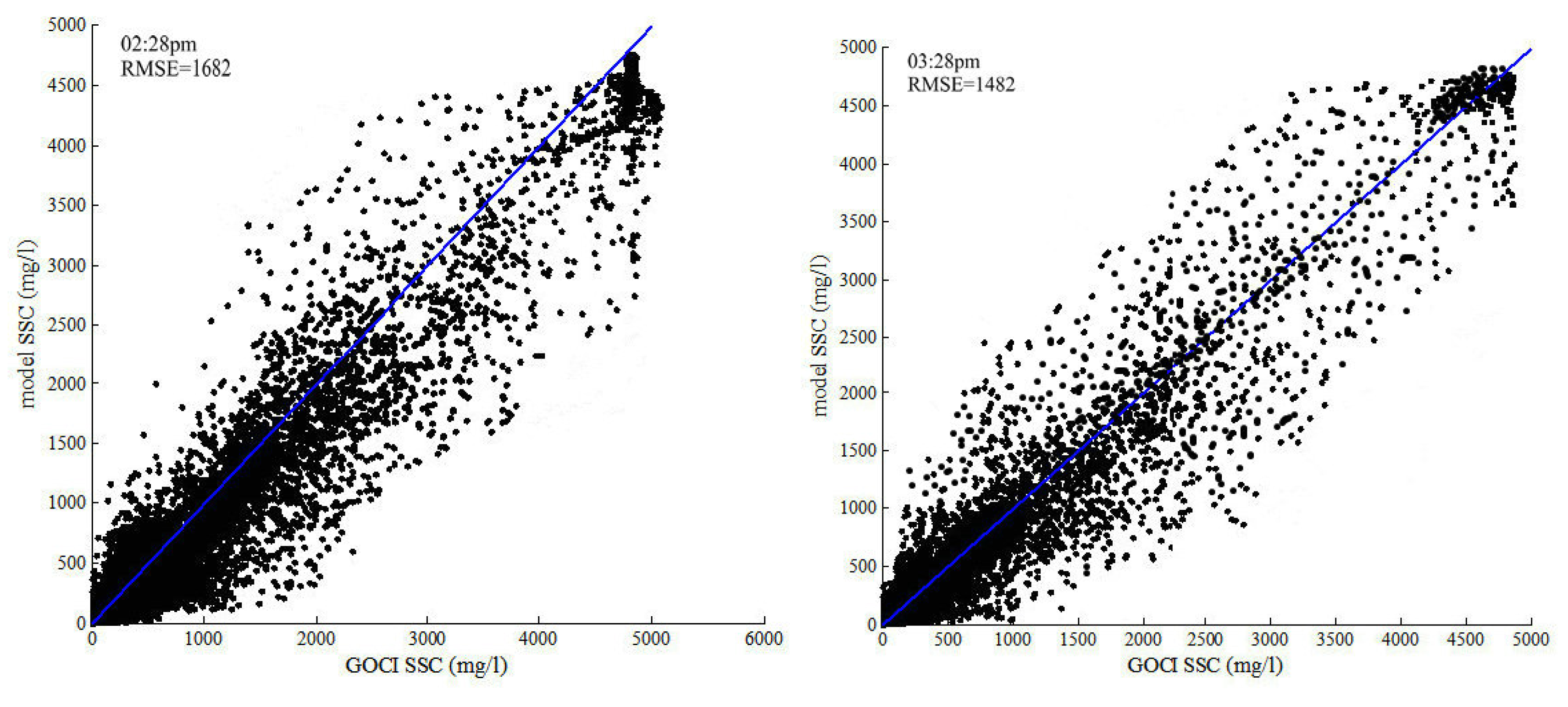
3.3. Improvements of Model/Satellite Comparisons
4. Conclusions
Acknowledgments
Author Contributions
Conflicts of Interest
References
- Mao, Z.; Chen, J.; Pan, D.; Tao, B.; Zhu, Q. A regional remote sensing algorithm for total suspended matter in the East China Sea. Remote Sens. Environ. 2012, 124, 819–831. [Google Scholar] [CrossRef]
- Doxaran, D.; Froidefond, J.-M.; Castaing, P.; Babin, M. Dynamics of the turbidity maximum zone in a macrotidal estuary (the Gironde, France): Observations from field and MODIS satellite data. Estuar. Coast. Shelf Sci. 2009, 81, 321–332. [Google Scholar] [CrossRef]
- Schlünz, B.; Schneider, R.R. Transport of terrestrial organic carbon to the oceans by rivers: Re-estimating flux- and burial rates. Int J. Earth Sci. 2000, 88, 599–606. [Google Scholar] [CrossRef]
- Yeshaneh, E.; Eder, A.; Blöschl, G. Temporal variation of suspended sediment transport in the Koga catchment, North Western Ethiopia and environmental implications. Hydrol. Process. 2014, 28, 5972–5984. [Google Scholar] [CrossRef]
- Chatanantavet, P.; Lamb, M.P. Sediment transport and topographic evolution of a coupled river and river plume system: An experimental and numerical study. J. Geophys. Res. F: Earth Surf. 2014, 119, 1263–1282. [Google Scholar] [CrossRef]
- Puls, W.; Doerffer, R.; Sundermann, J. Numerical simulation and satellite observations of suspended matter in the North Sea. Ocean. Eng. IEEE J. 1994, 19, 3–9. [Google Scholar] [CrossRef]
- Doxaran, D.; Lamquin, N.; Park, Y.-J.; Mazeran, C.; Ryu, J.-H.; Wang, M.; Poteau, A. Retrieval of the seawater reflectance for suspended solids monitoring in the East China Sea using MODIS, MERIS and GOCI satellite data. Remote Sens. Environ. 2014, 146, 36–48. [Google Scholar] [CrossRef]
- Ramakrishnan, R.; Rajawat, A.S. Simulation of suspended sediment transport initialized with satellite derived suspended sediment concentrations. J. Earth Syst. Sci. 2012, 121, 1201–1213. [Google Scholar] [CrossRef]
- Guillou, N.; Rivier, A.; Gohin, F.; Chapalain, G. Modeling Near-Surface Suspended Sediment Concentration in the English Channel. J. Mar. Sci. Eng. 2015, 3, 193–215. [Google Scholar] [CrossRef]
- Jensen, J.R.; Kjerfve, B.; Ramsey, E.W.; Magill, K.E.; Medeiros, C.; Sneed, J.E. Remote sensing and numerical modeling of suspended sediment in Laguna de Terminos, Campeche, Mexico. Remote Sens. Environ. 1989, 28, 33–44. [Google Scholar] [CrossRef]
- Ouillon, S.; Douillet, P.; Andréfouët, S. Coupling satellite data with in situ measurements and numerical modeling to study fine suspended-sediment transport: A study for the lagoon of New Caledonia. Coral Reefs 2004, 23, 109–122. [Google Scholar]
- Pleskachevsky, A.; Gayer, G.; Horstmann, J.; Rosenthal, W. Synergy of satellite remote sensing and numerical modeling for monitoring of suspended particulate matter. Ocean Dyn. 2005, 55, 2–9. [Google Scholar] [CrossRef]
- Gerritsen, H.; Vos, R.J.; van der Kaaij, T.; Lane, A.; Boon, J.G. Suspended sediment modelling in a shelf sea (North Sea). Coast. Eng. 2000, 41, 317–352. [Google Scholar] [CrossRef]
- Vos, R.J.; ten Brummelhuis, P.G.J.; Gerritsen, H. Integrated data-modelling approach for suspended sediment transport on a regional scale. Coast. Eng. 2000, 41, 177–200. [Google Scholar] [CrossRef]
- Fettweis, M.; Nechad, B.; Van den Eynde, D. An estimate of the suspended particulate matter (SPM) transport in the southern North Sea using SeaWiFS images, in situ measurements and numerical model results. Cont. Shelf Res. 2007, 27, 1568–1583. [Google Scholar] [CrossRef]
- Kunte, P.D.; Zhao, C.; Osawa, T.; Sugimori, Y. Sediment distribution study in the Gulf of Kachchh, India, from 3D hydrodynamic model simulation and satellite data. J. Mar. Syst. 2005, 55, 139–153. [Google Scholar] [CrossRef]
- Park, E.; Latrubesse, E.M. Modeling suspended sediment distribution patterns of the Amazon River using MODIS data. Remote Sens. Environ. 2014, 147, 232–242. [Google Scholar] [CrossRef]
- Sipelgas, L.; Raudsepp, U.; Kõuts, T. Operational monitoring of suspended matter distribution using MODIS images and numerical modelling. Adv. Space Res. 2006, 38, 2182–2188. [Google Scholar] [CrossRef]
- Chauhan, O.S.; Menezes, A.A.A.; Jayakumar, S.; Malik, M.A.; Pradhan, Y.; Rajawat, A.S.; Nayak, S.R.; Bandekar, G.; Almeida, C.; Talaulikar, M.; et al. Influence of the macrotidal environment on the source to sink pathways of suspended flux in the Gulf of Kachchh, India: Evidence from the Ocean Colour Monitor (IRS-p4). Int. J. Remote Sens. 2007, 28, 3323–3339. [Google Scholar] [CrossRef]
- Li, H.; Arias, M.; Blauw, A.; Los, H.; Mynett, A.E.; Peters, S. Enhancing generic ecological model for short-term prediction of Southern North Sea algal dynamics with remote sensing images. Ecol. Model. 2010, 221, 2435–2446. [Google Scholar] [CrossRef]
- Stanev, E.; Kandilarov, R. Sediment dynamics in the Black Sea: Numerical modelling and remote sensing observations. Ocean Dyn. 2012, 62, 533–553. [Google Scholar] [CrossRef]
- Luyten, P.J.; Jones, J.E.; Proctor, R.; Tabor, A.; Tett, P.; Wild-Allen, K. COHERENS–A Coupled Hydrodynamical-Ecological Model for Regional and Shelf Seas: User Documentation; MUMM Report; Management Unit of the Mathematical Models of the North Sea: Brussels, Belgium, 1999. [Google Scholar]
- Liu, J.P.; Xu, K.H.; Li, A.C.; Milliman, J.D.; Velozzi, D.M.; Xiao, S.B.; Yang, Z.S. Flux and fate of Yangtze River sediment delivered to the East China Sea. Geomorphology 2007, 85, 208–224. [Google Scholar] [CrossRef]
- Sternberg, R.W.; Larsen, L.H.; Miao, Y.T. Tidally driven sediment transport on the East China Sea continental shelf. Cont. Shelf Res. 1985, 4, 105–120. [Google Scholar] [CrossRef]
- Lin, C.-M.; Zhuo, H.-C.; Gao, S. Sedimentary facies and evolution in the Qiantang River incised valley, eastern China. Mar. Geol. 2005, 219, 235–259. [Google Scholar] [CrossRef]
- Milliman, J.D.; Meade, R.H. World-wide delivery of river sediment to the oceans. J. Geol. 1983, 91, 1–21. [Google Scholar] [CrossRef]
- Ahn, J.-H.; Park, Y.-J.; Ryu, J.-H.; Lee, B.; Oh, I. Development of atmospheric correction algorithm for Geostationary Ocean Color Imager (GOCI). Ocean Sci. J. 2012, 47, 247–259. [Google Scholar] [CrossRef]
- Choi, J.-K.; Park, Y.J.; Lee, B.R.; Eom, J.; Moon, J.-E.; Ryu, J.-H. Application of the Geostationary Ocean Color Imager (GOCI) to mapping the temporal dynamics of coastal water turbidity. Remote Sens. Environ. 2014, 146, 24–35. [Google Scholar] [CrossRef]
- Choi, J.-K.; Park, Y.J.; Ahn, J.H.; Lim, H.-S.; Eom, J.; Ryu, J.-H. GOCI, the world’s first geostationary ocean color observation satellite, for the monitoring of temporal variability in coastal water turbidity. J. Geophys. Res.: Oceans 2012, 117. [Google Scholar] [CrossRef]
- Ryu, J.-H.; Han, H.-J.; Cho, S.; Park, Y.-J.; Ahn, Y.-H. Overview of geostationary ocean color imager (GOCI) and GOCI data processing system (GDPS). Ocean Sci. J. 2012, 47, 223–233. [Google Scholar] [CrossRef]
- He, X.; Bai, Y.; Pan, D.; Tang, J.; Wang, D. Atmospheric correction of satellite ocean color imagery using the ultraviolet wavelength for highly turbid waters. Opt. Express 2012, 20, 20754–20770. [Google Scholar] [CrossRef] [PubMed]
- He, X.; Bai, Y.; Pan, D.; Huang, N.; Dong, X.; Chen, J.; Chen, C.-T.A.; Cui, Q. Using geostationary satellite ocean color data to map the diurnal dynamics of suspended particulate matter in coastal waters. Remote Sens. Environ. 2013, 133, 225–239. [Google Scholar] [CrossRef]
- Liang, B.-C.; Li, H.-J.; Lee, D.-Y. Bottom shear stress under wave-current interaction. J. Hydrodyn. Ser. B 2008, 20, 88–95. [Google Scholar] [CrossRef]
- Marinov, D.; Norro, A.; Zaldívar, J.-M. Application of COHERENS model for hydrodynamic investigation of Sacca di Goro coastal lagoon (Italian Adriatic Sea shore). Ecol. Model. 2006, 193, 52–68. [Google Scholar] [CrossRef]
- Shi, J.Z.; Li, C.; Dou, X.-P. Three-dimensional modeling of tidal circulation within the north and south passages of the partially-mixed Changjiang River Estuary, China. J. Hydrodyn. Ser. B 2010, 22, 656–661. [Google Scholar] [CrossRef]
- Guillou, N.; Chapalain, G. Modelling impact of northerly wind-generated waves on sediments resuspensions in the Dover Strait and adjacent waters. Cont. Shelf Res. 2011, 31, 1894–1903. [Google Scholar] [CrossRef]
- Mellor, G.L.; Yamada, T. Development of a turbulence closure model for geophysical fluid problems. Rev. Geophys. 1982, 20, 851–875. [Google Scholar] [CrossRef]
- Smagorinsky, J. General circulation experiments with the primitive equations. Mon. Weather Rev. 1963, 91, 99–164. [Google Scholar] [CrossRef]
- Steinhorn, I. Salt flux and evaporation. J. phys. Oceanogr. 1991, 21, 1681–1683. [Google Scholar] [CrossRef]
- Moon, I.-J. Impact of a coupled ocean wave–tide–circulation system on coastal modeling. Ocean Model. 2005, 8, 203–236. [Google Scholar] [CrossRef]
- Jiang, W.; Pohlmann, T.; Sun, J.; Starke, A. SPM transport in the Bohai Sea: Field experiments and numerical modelling. J. Mar. Syst. 2004, 44, 175–188. [Google Scholar] [CrossRef]
- Zhu, Y.; Chang, R. Preliminary study of the dynamic origin of the distribution pattern of bottom sediments on the continental shelves of the Bohai Sea, Yellow Sea and East China Sea. Estuar. Coast. Shelf Sci. 2000, 51, 663–680. [Google Scholar] [CrossRef]
- DeMaster, D.J.; McKee, B.A.; Nittrouer, C.A.; Jiangchu, Q.; Guodong, C. Rates of sediment accumulation and particle reworking based on radiochemical measurements from continental shelf deposits in the East China Sea. Cont. Shelf. Res. 1985, 4, 143–158. [Google Scholar] [CrossRef]
- Feng, Y.-J.; Li, Y.; Xie, Q.-C.; Zhang, L.-R. Morphology and activity of sedimentary interfaces of the Hangzhou Bay. Acta Oceanol. Sin. 1990, 12, 213–223. [Google Scholar]
- Jiyu, C.; Cangzi, L.; Chongle, Z.; Walker, H.J. Geomorphological development and sedimentation in Qiantang Estuary and Hangzhou Bay. J. Coast. Res. 1990, 6, 559–572. [Google Scholar]
- Xie, D.; Wang, Z.; Gao, S.; De Vriend, H.J. Modeling the tidal channel morphodynamics in a macro-tidal embayment, Hangzhou Bay, China. Cont. Shelf Res. 2009, 29, 1757–1767. [Google Scholar] [CrossRef]
- Jones, S.; Jago, C.; Simpson, J. Modelling suspended sediment dynamics in tidally stirred and periodically stratified waters: Progress and pitfalls. Mix. Estuaries Coast. Seas 1996, 50, 302–324. [Google Scholar]
- Lee, C.; Schwab, D.J.; Beletsky, D.; Stroud, J.; Lesht, B. Numerical modeling of mixed sediment resuspension, transport, and deposition during the March 1998 episodic events in southern Lake Michigan. J. Geophys. Res.: Oceans 2007, 112. [Google Scholar] [CrossRef]
- Peckham, S.D. A new method for estimating suspended sediment concentrations and deposition rates from satellite imagery based on the physics of plumes. Comput. Geosci. 2008, 34, 1198–1222. [Google Scholar] [CrossRef]
- Winterwerp, J.C. A simple model for turbulence induced flocculation of cohesive sediment. J.Hydraul. Res. 1998, 36, 309–326. [Google Scholar] [CrossRef]


© 2016 by the authors; licensee MDPI, Basel, Switzerland. This article is an open access article distributed under the terms and conditions of the Creative Commons by Attribution (CC-BY) license (http://creativecommons.org/licenses/by/4.0/).
Share and Cite
Yang, X.; Mao, Z.; Huang, H.; Zhu, Q. Using GOCI Retrieval Data to Initialize and Validate a Sediment Transport Model for Monitoring Diurnal Variation of SSC in Hangzhou Bay, China. Water 2016, 8, 108. https://doi.org/10.3390/w8030108
Yang X, Mao Z, Huang H, Zhu Q. Using GOCI Retrieval Data to Initialize and Validate a Sediment Transport Model for Monitoring Diurnal Variation of SSC in Hangzhou Bay, China. Water. 2016; 8(3):108. https://doi.org/10.3390/w8030108
Chicago/Turabian StyleYang, Xuefei, Zhihua Mao, Haiqing Huang, and Qiankun Zhu. 2016. "Using GOCI Retrieval Data to Initialize and Validate a Sediment Transport Model for Monitoring Diurnal Variation of SSC in Hangzhou Bay, China" Water 8, no. 3: 108. https://doi.org/10.3390/w8030108