Responses of Sediment Yield to Vegetation Cover Changes in the Poyang Lake Drainage Area, China

Abstract

Ascertaining the relationships between sediment transport processes and vegetation cover is essential for watershed soil and water conservation. However, it is not easy to realize this target on a large scale. In this study, the location-weighted landscape contrast index (LCI) based on the “source-sink” theory of ecological processes was introduced to unravel the response of sediment yield to vegetation cover changes in the Poyang Lake drainage area (the largest freshwater lake in China). A modified location-weighted landscape contrast index (mLCI) was proposed to improve the accuracy and efficiency of the LCI. The average vegetation fraction of the study area significantly increased from 46.2% in Period I (1992–1994) to 76.5% in Period II (2004–2006) and then slightly decreased to 73.2% in Period III (2011–2013). From Period I to Period II, the area-specific sediment yield (ASY) sharply decreased by 55%. In Period II, the “source” vegetation patches were found further away from the water bodies, and were more likely to be located on gentler slopes than in Period I. From Period II to Period III, the ASY sharply increased by 83%. In Period III, “source” patches were found closer to the water bodies than in Period II, whereas the “sink” patches were found further away from the water bodies. The high statistical correlation between LCIs/mLCIs and ASY indicated a sensitive response of the sediment yield to vegetation cover changes that significantly altered the sediment transport processes in the study area. The ASY was better correlated with the mLCI than with the LCI. Three key harnessing sub-watersheds of the Ganjiang watershed were identified by calculating the mLCIs: Qingfengshan, Yuanhe, and Jinjiang. This study supported watershed ecological management in the Poyang Lake drainage area and provided a methodology reference for future sediment transport process studies.

1. Introduction

Sediment loss by water is a serious environment problem that is threatening the sustainability of ecological system [1]. The Poyang Lake drainage area (covering 122,100 km²) has contributed greatly to the socioeconomic development of China. However, this region has a fragile ecosystem [2]. The dominant soil type in this region belongs to red soil with a low infiltration rate, which can prompt surface runoff and sediment fluxes [3]. Previous studies indicated that serious soil erosion by water caused severe environmental degradation in the Poyang Lake drainage area [4,5]. For decades, this region has exhibited the severest soil erosion in south China [4]. The area of soil erosion occupies approximately 20.03% of the total territory, and 99.45% of the soil erosion is caused by water erosion [6]. In recent years, the annual amount of sediment yield discharged into Poyang Lake reached 12 million metric tons, with a mean bottom accretion rate of up to 3 mm/a [7]. The regulation and storage functions of Poyang Lake have gradually reduced.

Vegetation cover exerts a significant influence on runoff-sediment transportation processes [8,9,10,11,12]. Over the past few decades, the Poyang Lake drainage area has experienced a significant change in vegetation coverage [13]. Developing an accurate and highly efficient method to elucidate the relationship between vegetation cover changes and sediment transportation processes is of practical significance for watershed management in this region. Manual field monitoring can provide fundamental data to reveal ecological processes associated with landscape changes. However, the use of this approach on a large scale requires a great expenditure of manpower and time.

During the last two decades, ecologists have achieved great progress in landscape spatial data acquisition and improved methods for quantitative analysis using readily accessible remote sensing data and significant advances in GIS technology. From a landscape ecological perspective, the ecological function of landscape patterns is often studied by investigating the statistical relationships between landscape indices and ecological conditions (e.g., exposure to contaminants, diversity and biological balance and physical/chemical attributes) [10,14,15]. The patch area, patch shape index, Shannon–Weaver diversity index, dominance index, and fragmentation index are commonly used landscape indices at both the slope and catchment (or regional) scales [8,16,17,18,19,20]. However, with the development of landscape ecology, elucidating ecological processes and their interactions with landscape patterns has become the focus of recent landscape ecology studies [21,22,23]. These landscape indices only take into account the composition and spatial configuration of the land cover and do not provide insights into the ecological processes [8,10]. Some landscape indices have been established from an ecological process perspective. For example, Borselli et al. [24] established an index of connectivity (IC) that represented a connectivity assessment based on information from the landscape. Mayor et al. [25] derived a spatial index (Flowlength) to quantify the connectivity in runoff source areas considering both the topography and vegetation pattern. These indices effectively address the runoff-sediment process. However, they are both heavily dependent on high-resolution spatial data and thus are not suitable for large-scale studies.

Chen et al. [8,26] established the location-weighted landscape contrast index (LCI) (see the methodology section for a thorough description of this method) to represent the ecological functions of landscape patterns based on the “source-sink” theory which has been commonly used to address the response of ecological process to landscape pattern changes [27,28]. Remarkably, the LCI is scale-independent (suitable for different sized watersheds) and regards not only the spatial configuration of the landscape but also the topographical characteristics of each land patch. Its advantages could also benefit from the readily available input data (low cost and wide coverage remote sensing images). Additionally, the series software ArcGIS provides a convenient environment for data processing. Previous studies employing the LCI primarily focused on NPS processes [29]. For example, Yue et al. [30] applied the LCI to analyze the influence of “source” and “sink” landscape spatial changes based on the total nitrogen (TN) and total phosphorus (TP) contents to assess water body quality in Shenzhen city, China. Liu et al. [31] studied the effects of land cover patterns on TN and TP in nine typical districts of the upper reaches of the Yangtze River using the LCI. These two studies both found that the LCI effectively quantified the contributions of landscape patterns to NPS processes at the watershed scale.

In a watershed, sediments generated from “source” land patches under the exogenic force (e.g., water flow) will be transported into water body (eventually exported out of the watershed) with part or all of them retarded by “sink” land patches. If the pattern of “source” and “sink” patches changes, the sediment yield observed at the outlet of the watershed should respond. Under this hypothesis, we applied the LCI to investigate the response of sediment yield to vegetation cover in the Poyang Lake drainage area, and addressed the following research questions: (1) What are the change characteristics of vegetation patterns related to topography in the study area? (2) How does the sediment yield respond to vegetation patterns changes? (3) Are there any critical sediment loss sub-watersheds that required special attention in the study area?

2. Study Area and Data

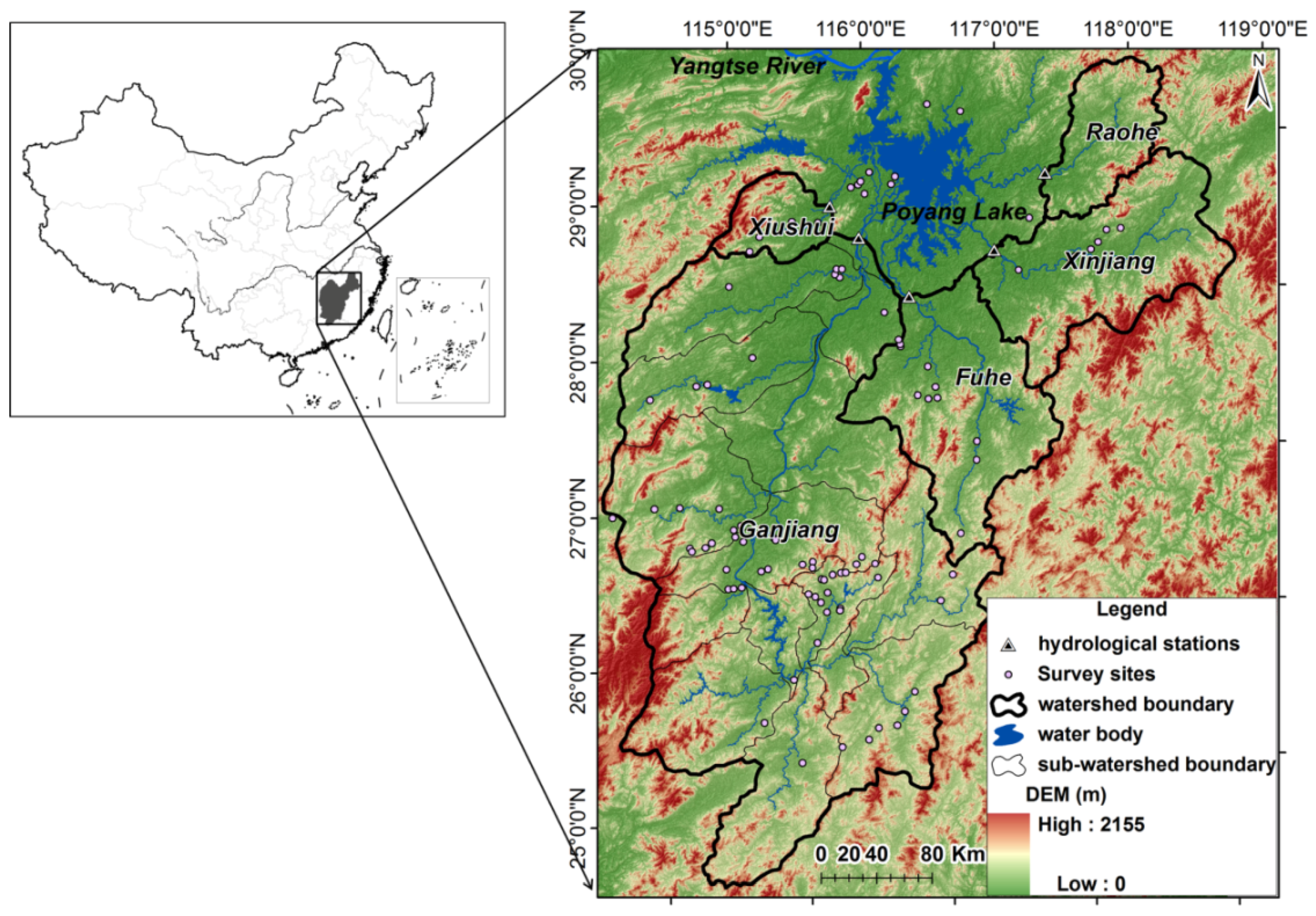
2.1. Study Area Description

The Poyang Lake drainage area consists of five river watersheds and the lake region (Poyang Lake and its vicinity areas). We selected five river watersheds (Ganjiang, Xiushui, Fuhe, Xinjiang and Raohe) as the study area. Each watershed is named after its chief river. As shown in Figure 1, the study area is distributed between 113°45′ and 118°35′ E longitude and 24°32′ and 29°36′ N latitude. These five rivers all flow into the largest freshwater lake in China (Poyang Lake), and eventually into the Yangtze River (Changjiang). The hydrological station names and locations can be identified by combining the information in Figure 1 and

Table 1. Mean annual area-specific sediment yield (ASY, t/(km²·a); a indicates the year) and the mean annual rainfall erosivity (MAE, (MJ·mm)/(km²·h·a)) in each watershed.

Watershed	Hydrological Stations	Watershed Area (×104 km2)	Period I (1992–1994)		Period II (2004–2006)		Period III (2011–2013)
			ASY	R	ASY	R	ASY	R
Ganjiang	Waizhou	8.09	103.4	10,252.9	44.62	10,112.5	23.82	9859.6
Fuhe	Lijiadu	1.58	105.5	10,225.3	51.05	11,260.1	72.09	10,195.3
Xinjiang	Meigang	1.55	167.7	11,671.6	53.18	10,852.0	75.94	10,686.4
Raohe	Hushan	0.64	40.6	11,852.6	31.56	10,210.5	195.68	12,250.8
Xiushui	Wanjiabu	0.35	110.4	10,525.9	54.19	9999.7	63.71	10,029.1

. The Ganjing watershed contains fifteen sub-watersheds. Nevertheless, these sub-watersheds lack hydrology measurements and the sediment yield data are inaccessible. The whole study area covers 122,100 km² and is characterized by a typical moist, subtropical climate with an average annual temperature of 17.7 °C, an average annual rainfall of 1786 mm and a maximum daily temperature of approximately 40 °C. The distribution of annual precipitation is uneven, with approximately 50% occurring in the summer when the temperature is relatively high. The north and min-north part of the study area has the lowest elevation, with smoothly undulating hilly lands and flat alluvial plains as the predominate relief accounting for approximately 35% of the total area. With mountains on the other three sides, the whole shape of the territory resembles a “dustpan”. The whole study area has symmetrical vegetation coverage. The vegetation fraction in the flat plains with high human disturbance is low. In contrast, the mountain areas are usually covered by thick forests. The dominant soil that is widely distributed in the region belongs to red soil developed from quaternary sediments. This type of soil has a low precipitation infiltration rate, and is degraded and erosion-prone [3]. Due to the possibility of severe soil loss, several soil and water conservation measures have been implemented. The most famous is the Grain-for-Green Program that promotes ecological reconstruction via the conversion of steeply sloped farmland into forest and grass [13]. At present, the sediment loss in the mountain areas covered by a high vegetation fraction is under control [4].

2.2. Data Sources and Processes

2.2.1. Rainfall Erosivity and Sediment Yield Data

The LCI does not consider the effects of rainfall variation on sediment loss. Therefore, to evaluate the relationship between vegetation cover changes and sediment loss, rainfall variation needed to be eliminated prior to the implementation of our study. We used rainfall erosivity to represent the ability of rainfall to cause soil erosion by considering the rainfall amount and intensity [32]. Based on the annual spatial data products of rainfall erosivity (1980–2014) developed by Xiao et al. [33] using the daily precipitation dataset provided by the China Meteorological Data Sharing Service System (http://cdc.nmic.cn/home.do), we investigated the annual rainfall erosivity trends in the five watersheds (Ganjiang, Xiushui, Fuhe, Xinjiang and Raohe) during the 34 year period. As shown in Table 1, three time periods (1992–1994, 2004–2006, and 2011–2013) with similar mean annual rainfall erosivities (MAEs) were selected. The MAE values exhibited in Table 1 had an average of 10,665.6 (MJ·mm)/(km²·h·a) and a standard deviation (SD) of 753.0 (MJ·mm)/(km²·h·a). The relative change between each MAE value and the average value did not exceed ±10% with the exception of Raohe in Period III (14%). In contrast, the MAE values in the other periods (one period = three years) that were not selected varied greatly (SD = 1404.1 (MJ·mm)/(km²·h·a)) and were not close to the MAE in the selected periods. We believed that the sediment yield changes among these three study periods were primarily caused by changes in the underlying surface rather than rainfall. To increase the representativeness and eliminate the random deviation, the area-specific sediment yield (ASY, the ratio of total sediment yield to the watershed area) and rainfall erosivity for the time Periods I, II and III were included as three-year average values. For example, we used the mean annual ASY over 1992–1994 to represent the situation in Period I. The corresponding sediment yield data from the five watersheds were extracted from the Changjiang sediment bulletins [34,35,36,37,38,39] and the study of Sun et al. [40]. This sediment yield data were observed by the hydrological stations located at the outlet of each watershed.

2.2.2. Remote Sensing Products

The MODIS 16-day vegetation index (VI) products (MOD13Q1 with a spatial resolution of 250 m) of Period II and Period III were obtained from the Goddard Space Flight Center (GSFC) (https://ladsweb.nascom.nasa.gov/index.html). All of the VI products used in our study were collected on the same Julian day (257) when the vegetation was at its utmost luxuriance. Landsat-5 Thematic Mapper (TM) images (with a spatial resolution of 30 m) were obtained from the Institute of Remote Sensing and Digital Earth (IRSD) (http://ids.ceode.ac.cn/query.html) to produce the VI for Period I. The acquisition day for all of the TM images applied in our study was near the Julian day of the MOD13Q1 products. The two sub-pixel model was applied to produce the vegetation fraction (VF) based on the VI products. The details are available in study of Miao et al. [41]. We calculated the three-year average VF value for each time period. For convenience, the VF of the study area was classified into five levels: high, moderately high, moderate, moderately low, and low (≥80%, 60%–80%, 40%–60%, 20%–40%, and <20%, respectively). The Shuttle Radar Topography Mission (SRTM) version 2 data were obtained from the Jet Propulsion Laboratory (http://srtm.csi.cgiar.org/SELECTION/inputCoord.asp). All spatial raster data were resampled into 250 m to unify the spatial resolution (Figure 2).

3. Methodology

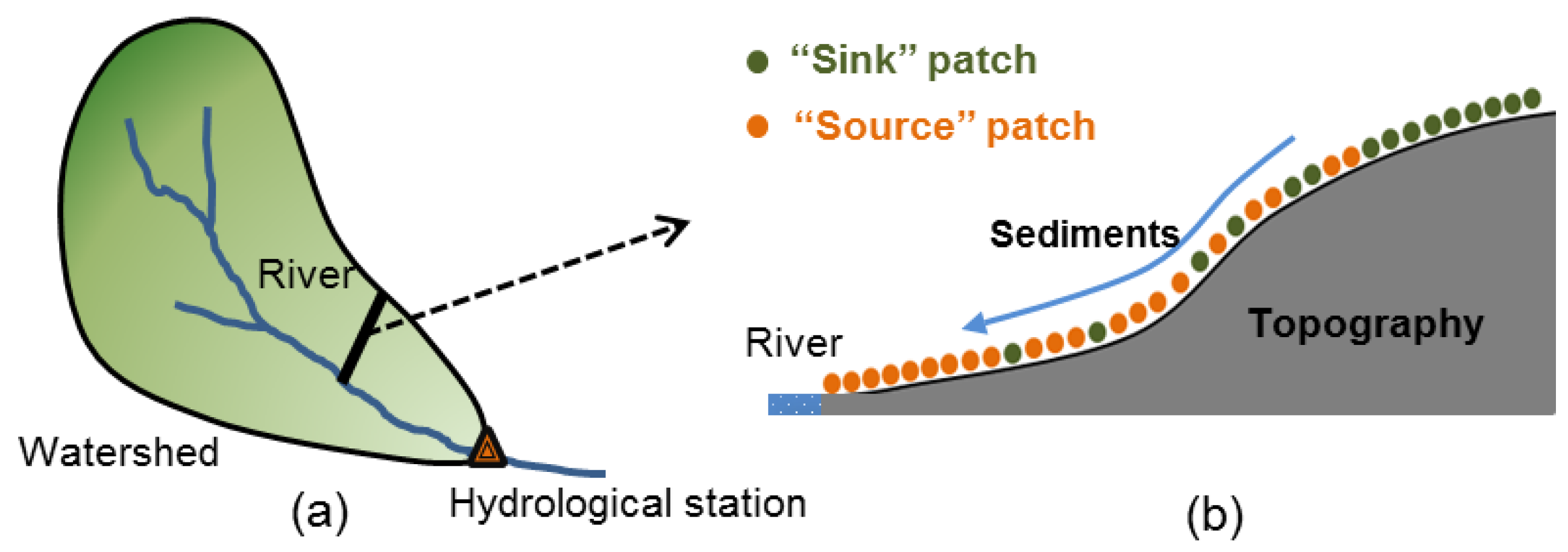
3.1. The “Source-Sink Theory” of Sediment Transport

The “source-sink” theory refers to the function of the “source” and the “sink” exerted by the landscape [8]. When integrated with a specific ecological process (sediment transport), “source” landscapes are those that can promote sediment production and transport, whereas “sink” landscapes refer to those that can retard or delay sediment transport. Naturally, “sink” landscapes belong to land patches with high vegetation fractions (e.g., forestland) that can effectively reduce sediment loss [42]. Notably, “sink” landscapes may not arrest all sediment. In other word, sediments may pass the “sink” landscapes with only part of them arrested. As shown in Figure 3, sediments generated from “source” land patches will be transported into the river (eventually exported out of the watershed) with part or all of them arrested by “sink” land patches. Theoretically, if the spatial distribution of the “source” and “sink” landscapes is balanced and reasonable, less sediment will be transported into the river, and a lower sediment yield will be observed by the hydrological station at the outlet of the watershed. Based on this theory, the LCI index could be suitable to evaluate the rationality of the landscape distribution aimed at sediment conservation by considering the area of the “source” and “sink” landscapes and their topography-related patterns as well as their efficiency of generating or arresting sediments. If the correlation coefficient of the LCI and sediment yield at the outlet of the watershed passes the significance testing, the LCI index possesses practicability.

3.2. Determination of the “Source” and “Sink” Patches

Land patches with high VF can reduce the sediment transport process, whereas those with low VFs are more likely to be eroded. Therefore, vegetation coverage can highly represent the land patch conditions that influence sediment transport process [10,11,12]. In our study, the VF produced in Section 2.2.2 was used to distinguish the “source” and “sink” land patch types. In October 2013, we performed a field survey of the study area. An accumulated survey length of 3063 km that included 1336 photos and a total of 93 patches with latitude and longitude information were recorded in the field survey database (Figure 1). Based on this data, we determined that a VF of approximately 60% could be considered the threshold at which the sediment transport process was effectively reduced. This finding coincided with the studies of Yuan et al. [43] and Wu et al. [44]. Hence, land patches with high and moderately high VFs were categorized as “sink” types, and land patches with low, moderately low and moderate VFs were categorized as “source” types. As shown in the Results Section, this threshold proved to be rational. However, it is essential to emphasize that the threshold is related to the specific vegetation cover and the sediment transport processes in the Poyang Lake drainage area, and cautions should be taken when extending this threshold to other regions.

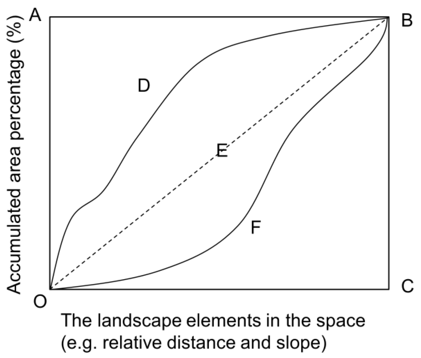
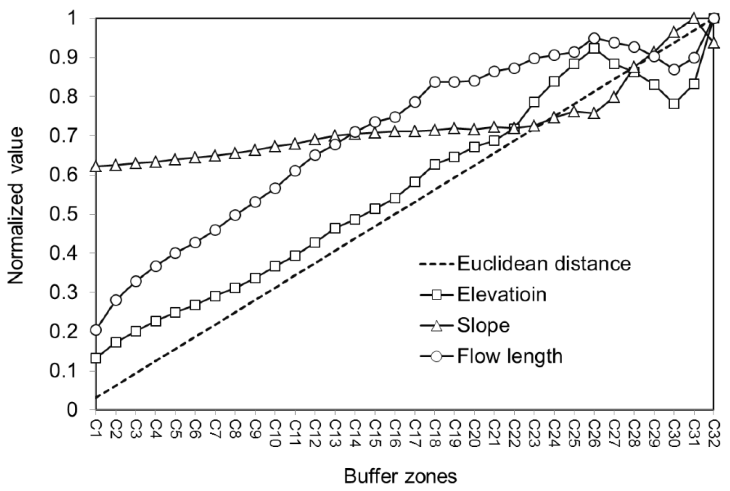
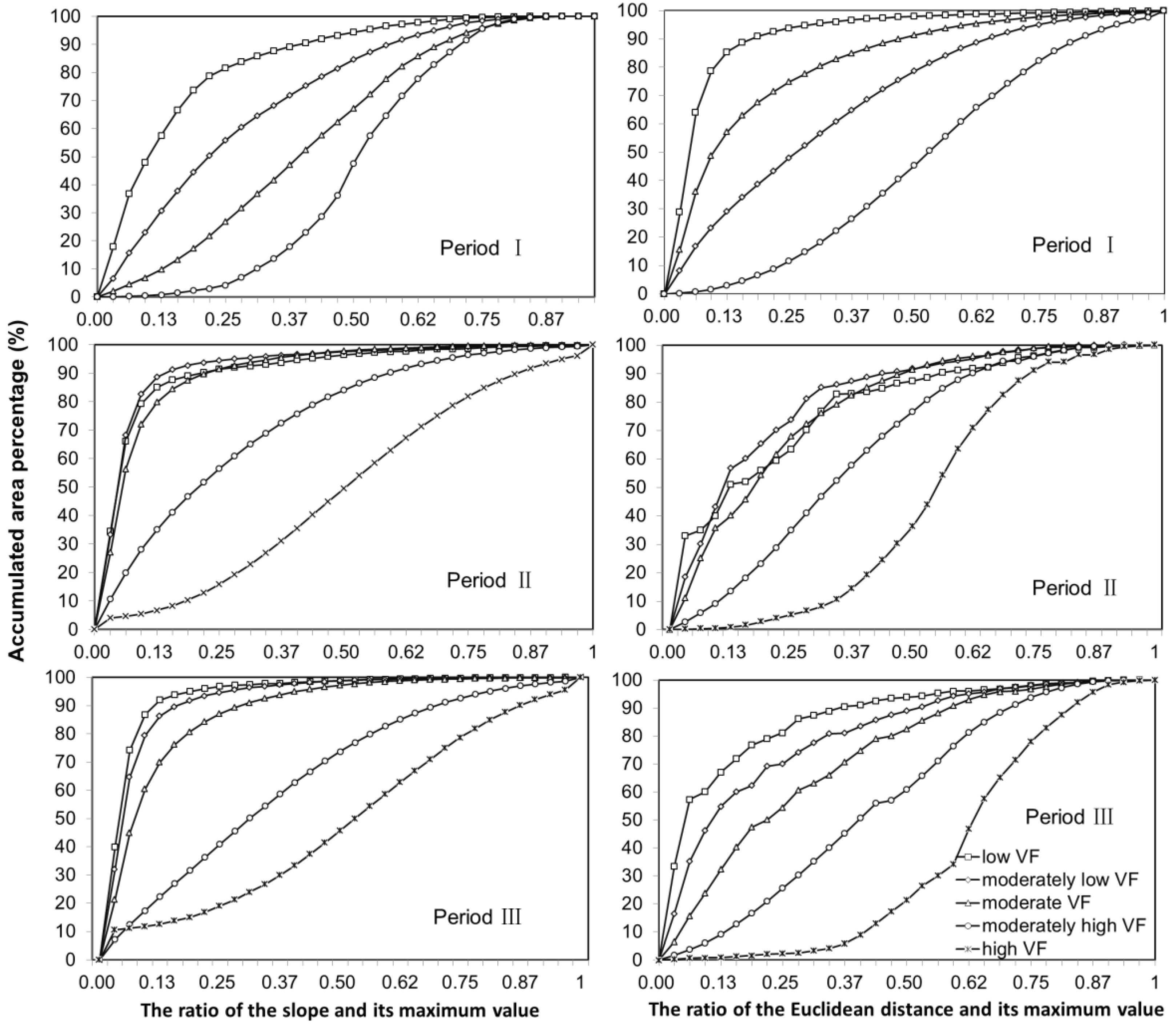
3.3. Description of the Topographical-Related Spatial Patterns of “Source” and “Sink”

The topography characteristics of land patches can be important factors that influence sediment transportation on terrestrial surfaces (e.g., elevation, slope, and flow length) [10,11,12,45,46]. Theoretically, sediments generated from “source” land patches with a shorter flow length have a greater chance of being transported into water body, thereby contributing to a higher sediment yield at the watershed outlet. The “sink” patches that are distributed near the water body have greater chance to arrest sediment than ones far from water body. Elevation and distance to water have similar functions with regards to flow length. Nevertheless, a steeper slope can enhance sediment transportation [47] and have an opposing function to elevation and distance to water. Simply speaking, a steeper slope, lower elevation and shorter flow length and distance to water result in a greater influence of “source” or “sink” land patches on the promotion or reduction of the sediment yield loss.

The Lorenz curve was applied to depict the topographical distribution characteristics of the “source” and “sink” land patches in a watershed (Figure 4). Using the distance to water as an example, O indicates the water body (e.g., river; distance = 0), C indicates the maximum distance, OC represents the increasing process of distance to water, OA is the corresponding accumulated area percentage of a type of “source” or “sink” land patch, ODBC refers to a Lorenz curve of a type of “source” or “sink” land patch that is primarily distributed near the water body and thus has more influence of the promotion or reduction of the sediment yield in water, OFBC is a case opposite to ODBC, and OEBC represents an even distribution case. Consequently, the area of the irregular polygon (A) encompassed by the Lorenz curve of a type of “source” or “sink” land patch is proportional to its influence on the sediment yield observed at the hydrological station at the outlet of the watershed.

We can calculate the total A of the “source” patches (three types) in a watershed as follow:

$$A_{source}={{\displaystyle \sum }}_{i=1}^M{{\displaystyle \int }}_{x=0}^C{R}_{xi}dx(i=1,2,3)$$

(1)

and that of the “sink” (two types) as follow:

$$A_{sink}={{\displaystyle \sum }}_{j=1}^N{{\displaystyle \int }}_{x=0}^C{S}_{xi}dx(j=1,2)$$

(2)

where C is the maximum value of the topographical index. Using the distance to water between the land patches and water body as an example; R_xi and S_xj indicate the accumulated areal percentages of the Lorenz curves of the “source” and “sink” land patch types, respectively; and M and N represent the numbers of the “source” and “sink” land patch types in the watershed, respectively.

A contrast index (CI) can be established to assess the balanced states of the “source” and “sink” patches in a watershed:

$$CI=A_{source}/A_{sink}={\displaystyle \sum }_{i=1}^M\underset{x=0}{\overset{C}{{\displaystyle \int }}}{R}_{xi}dx/{\displaystyle \sum }_{j=1}^N\underset{x=0}{\overset{C}{{\displaystyle \int }}}{S}_{xj}dx$$

(3)

When CI > 1, the “source” patches are more likely to be distributed near the water than the “sink” patches, and thus contribute more to the sediment loss. When CI < 1, the effect is opposite to the case of CI > 1. When CI = 1, the spatial distribution of the “source” and “sink” landscapes is balanced.

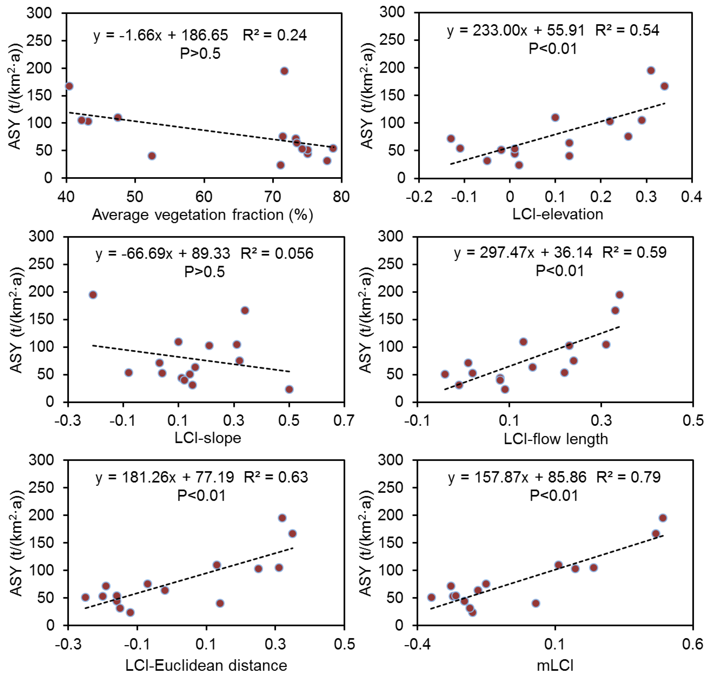
3.4. Location-weighted landscape contrast index

In addition to the topography-related patterns, the “source” and “sink” patch areas in a watershed and their efficiency in generating or arresting sediments are important for the sediment transport process. By considering the latter two factors, the final LCI calculation formula aimed at the sediment transport process in a watershed can be written as:

$$\text{LCI}=\log \left\{{\displaystyle \sum }_{i=1}^M\underset{x=0}{\overset{C}{{\displaystyle \int }}}{R}_{xi}dx\times {\phi }_i\times p_i/{\displaystyle \sum }_{j=1}^N\underset{x=0}{\overset{C}{{\displaystyle \int }}}{S}_{xj}dx\times {\phi }_j\times p_j\right\}$$

(4)

where ${\phi }_i$ and ${\phi }_j$ are the effectiveness parameters of promoting and preventing sediment transport by the “source” and “sink” land patch types, respectively; and $p_i$ and $p_j$ represent the area percentages of the “source” and “sink” land patch types in the watershed, respectively. When LCI = 0, the “source” and “sink” patches reach a balance. When LCI > 0, the contribution of the “source” is greater than the contribution of the “sink”, and the vegetation cover in the watershed tends to generate and transport sediments. When LCI < 0, the situation is reversed.

The accurate determination of ${\phi }_i$ and ${\phi }_j$ can be difficult. We used the vegetation coverage and management factor (C) that were usually implemented in USLE and its revised form RUSLE to approximately represent the effectiveness of the “source” land patch type parameter. The ${\phi }_i$ of the moderate, moderately low and low VFs was set at 0.15, 0.2 and 0.4, respectively, according to the relevant achievements of the C values for the different VF levels [48,49]. Considering the opposing meanings of ${\phi }_i$ and ${\phi }_j$, we assumed that the functions of a high VF in reducing sediment and a low VF in causing sediment could be approximately counterbalanced; a similar assumption was made concerning a moderately high VF versus a moderately low VF. Thus, the ${\phi }_j$ values of a high VF and a moderately high VF were set at 0.4 and 0.2, respectively.

3.5. A modified Topographic Index

In previous ecological process studies using the LCI, the commonly considered topographical indices (e.g., elevation, slope, flow length, and distance to water) were individually introduced into the LCI calculation. However, some indices, such as elevation, flow length, and distance to water, are highly correlated in most cases (Figure 5), which always leads to similar LCI results [30,31,50]. This factor may result in redundancy and reduce the research efficiency. In this study, we proposed a modified topographical index that combine the two topographical indices with relatively low spatial correlativity in the hope of improving the LCI and the research efficiency. The Euclidean distance (ED) to water was applied to replace the elevation and flow length. The slope had an opposing function compared to the sediment transport process to ED and was processed into the modified index. The modified ED (mED) index can be expressed as:

$$\text{mED}=\left(1+\frac{D}{D_{max}}\right)\times \left(1-\frac{S}{S_{max}}\right)$$

(5)

where D is the Euclidean distance from land patches to water; ${\mathrm{D}}_{\text{max}}$ is the farthest Euclidean distance in a given watershed; S is the slope; and ${\mathrm{S}}_{\text{max}}$ is the maximum slope in a given watershed. We introduce mED into Equation (4) to calculate the modified location-weighted landscape contrast index (mLCI), and test its applicability by comparing it with LCI-elevation, LCI-slope, LCI-flow length, and LCI-Euclidean distance. All of the topographical indices utilized in this study were produced in the GIS environment based on the SRTM-DEM data.

4. Results

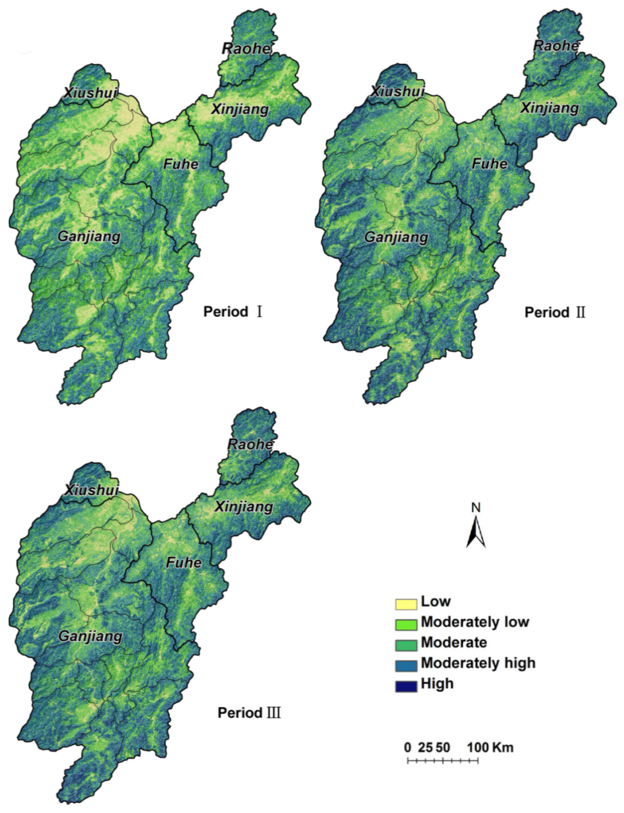
4.1. Temporal and Spatial Variations in Vegetation Covers

Figure 2 exhibits the VF distribution of the study area in the three time periods (1992–1994, 2004–2006, and 2011–2013). The average VFs of the study area in these three periods were 46.2%, 76.5%, and 73.2%, respectively. All of the watersheds (Ganjiang, Xiushui, Fuhe, Xinjiang and Raohe) experienced a sharp increase and then a slight decrease in the average VF (

Table 2. Areal percentages of the five vegetation fraction (VF, %) levels in each watershed.

Watershed	Period	VF Levels
		Low	Moderately Low	Moderate	Moderately High	High
Ganjiang	I	7.55	23.1	59.23	10.04	0.08
	II	1.54	5.2	23.02	53.32	16.92
	III	2.52	5.95	24.21	57.98	9.34
Fuhe	I	7.81	25.29	61.05	5.79	0
	II	1.17	3.52	20.34	61.94	13.04
	III	2.42	5.52	25.02	63.37	3.68
Xinjiang	I	9.53	27.05	60.18	3.24	0.01
	II	1.2	4.05	18.23	55.50	21.01
	III	2.21	7.04	29.3	56.02	5.4
Raohe	I	2.53	5.46	35.94	45.85	10.22
	II	0.5	0.9	8.34	58.46	31.72
	III	1.28	13.67	25.25	46.56	13.24
Xiushui	I	2.05	14.62	37.45	45.03	0.85
	II	1.01	3.02	15.51	46.01	34.85
	III	1.4	6.01	25.37	56.6	10.62

). We investigated the spatial distribution characteristics of the five VF levels (high, moderately high, moderate, moderately low, and low) in all watersheds in the three periods. The Xinjiang watershed was selected as an example due to its strong representativeness. Taking into account the high spatial correction among the Euclidean distance, elevation, and flow length (Figure 5), slope and Euclidean distance were selected for the spatial distribution investigation of the VFs. As shown in Figure 6, there was no high VF level in Period I. “Source” VFs were more likely to be located on gentler slopes in Period II than in Period I. In Period II, “sink” VFs were also more likely to be located on gentler slopes than in Period I; however, the “sink” VFs were not as evident as the “source” VFs. In Period III, both “source” and “sink” patches (excluding high level) were more likely to be located on steeper slopes. With regards to the Euclidean distance to water, in Period II, the “source” VFs were found further away from the water bodies than in Period I. The curve of the moderately high VFs experienced almost no change from Period I to II. In Period III, the low VFs were found closer to the water bodies, whereas, the high VFs found further away from the water bodies than in Period II. Generally, the change in the spatial distribution of VFs increased the likelihood for sediment entrapment from Period I to Period II. Nevertheless, it decreased the likelihood for sediment entrapment to some extent during Period II to III.

4.2. LCI/mLCI Analysis in the Five Watersheds

When the LCIs/mLCIs, average VF and ASY of the five watersheds in the three periods were calculated, we investigated their coupling relationships using a scatter map (Figure 7). Theoretically, there should be a negative correlation between the average VF and ASY. As shown in Figure 7, the coefficient of determination (R²) yielded using linear regression analysis was −0.24, and did not pass the significance testing (p > 0.05). In contrast, the LCIs/mLCIs (with the exception of LCI-slope) exhibited a highly significant correlation with the ASY. Based on the LCI concept, the ASY not only responded to the change of proportion in the VF levels but also the change in their spatial patterns. Using the Xinjiang watershed as an example, from Period I to Period II, the ASY was sharply reduced from 167 to 53.1 t/(km²·a) (Figure 7). Accordingly, the watershed experienced a great improvement in vegetation coverage in these two time periods. The areal percentage of high and moderately high levels increased from 3.24% and 0.01% to 55.5% and 21.01%, respectively (Table 2). During the same time period, the changes in vegetation pattern of the Xinjiang watershed increased the likelihood for sediment entrapment, and thus prompted a sharp reduction in the ASY. From Period II to Period III, there was no evident change in the VF (Table 2). However, the increase in the ASY from 53.1 to 75.9 t/(km²·a) (Figure 7) was relatively remarkable. Therefore, the change in the vegetation patterns (which decreased the likelihood for sediment entrapment as seen in Section 4.1) should be awarded the most responsibility (refer to the Discussion Section for details). As mentioned above, a steeper slope can enhance the sediment generation of the “source” landscape. Theoretically, LCI-slope should have a negative correlation with the ASY. However, the vegetation patches with steeper slope were usually further away from the water bodes (Figure 5). Therefore, the negative correlation could be weakened (p > 0.05).

Generally, the ASY, which was highly related to the LCI/mLCI, showed a sensitive response to vegetation cover changes in the Poyang Lake drainage area. In comparison, we found that the mLCI considering the Euclidean distance modified by slope information had the best correlation with the ASY (R² = 0.79, p < 0.01). This result illustrates the advancement of the topographical index of the mED (Figure 8) established in the present study. We can also conclude that, compared to other LCIs (LCI-elevation, LCI-slope, LCI-flow length, and LCI-Euclidean distance), mLCI is the optimum index to indicate the sediment loss risk in the study area.

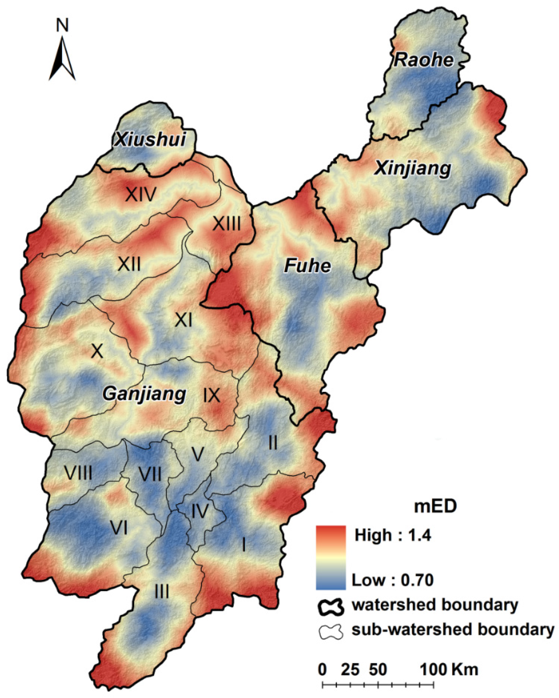
4.3. The mLCIs of the Sub-Watersheds of the Ganjiang Watershed

We applied the mLCIs as the judgment indices of sediment loss risk for the sub-watersheds of Ganjiang, where measurements of sediment yield are sparse. As shown in

Table 3. mLCIs in each sub-watersheds of Ganjiang.

Code	Sub-Watershed Name	mLCIs
		Period I	Period II	Period III
I	Lian-Mian	0.08	−0.31	−0.34
II	Meijiang	0.16	−0.27	−0.38
III	Taojiang	0.15	−0.22	−0.31
IV	Gongshui	0.11	−0.26	−0.27
V	Pingjiang	0.24	−0.15	−0.24
VI	Shangyou-Zhangshui	0.16	−0.27	−0.28
VII	Upper-Ganliu	0.22	−0.24	−0.30
VIII	Suichuanjiang	0.14	−0.66	−0.45
IX	Longjiang	0.23	−0.32	−0.3
X	Lu-He	0.05	−0.31	−0.29
XI	Enjiang	0.24	−0.24	−0.22
XII	Yuanhe	0.23	−0.28	−0.06
XIII	Qingfengshan	0.45	−0.07	0.04
XIV	Jinjiang	0.17	−0.22	−0.06

, Qingfengshan had the highest mLCI in the three periods (0.45, −0.07, and 0.04, respectively), followed by Yuanhe (0.23, −0.28, and −0.06, respectively) and Jinjiang (0.17, −0.22, and −0.07, respectively). The latter two watersheds showed a similar change trend in their mLCIs. These three sub-watersheds of Ganjiang should receive special attention for soil conservation. Sub-watersheds possessing relatively excellent soil conservation statuses were also identified. The mLCIs of Suichuanjiang, Meijiang, and Lian-Mian were lower than other sub-watersheds, and Suichuanjiang was characterized by the lowest mLCIs (0.14, −0.66, and −0.45 in Period I, II, and III, respectively).

5. Discussion

It is conceivable that vegetation cover can strongly influence the runoff process that transports the sediments into water (e.g., river) [10,11,12]. Indeed, the vegetation coverage conditions in the Poyang Lake drainage area changed significantly from Period I to Period III. This result may be partially due to the implementation of the “Grain for Green” program and the cultivated land balance policy [13,51,52]. Nevertheless, studying the response of sediment yield to vegetation cover change can promote the development of watershed management in the Poyang Lake drainage area.

The LCI index applied in our study is a comprehensive landscape index based on the “source-sink” theory of ecological processes. When the LCI is calculated, the contribution of “source” and “sink” land patches to the sediment loss in watershed is addressed. Therefore, the LCI could be directly related to the sediment yield observed at the outlet of the watershed. Our study confirmed the high accuracy of the LCI in reflecting the sediment yield. For example, there was a remarkable increase in the ASY (from 53.1 to 75.9 t/(km²·a), representing a 42.9% increase) in the Xinjiang watershed from Period II to Period III. However, the average vegetation fraction decreased by only 3.7%. Thus, the average vegetation fraction change provided a very limited explanation for the ASY change. We observed a remarkable topography-related vegetation pattern change: in Period III, the “source” patches were found closer to the water bodies than in Period II, whereas, the “sink” patches were found further away from the water bodies. This finding may be an important promoting factor for the increase in the ASY. The LCIs took into account vegetation pattern changes and thus presented a remarkable increase (all more than 44%) that responded sensitively to the increase in the ASY. The prominent coupling relationship between the LCIs/mLCIs and ASY confirmed our success in introducing the LCI to study sediment yield variations in response to vegetation cover changes in the Poyang Lake drainage area, China. The mLCIs proposed in this study (which performed better than the LCIs) were used to identify the critical sediment loss sub-watersheds.

Nevertheless, the limitations of the mLCI should be known prior to its application. As mentioned in Section 2.2.1, the mLCI does not consider the effects of rainfall variation on sediment transport processes. Thus, the mLCI may only be applicable for regions with similar precipitation conditions when studying the relationship between vegetation cover and sediment yield. For example, in this study, we selected three periods with similar rainfall erosivities. However, the erosivity of the Raohe watershed in Period III was relatively higher than of the other watersheds in the different periods. This discrepancy is why the LCI/mLCI and ASY did not correlate well in the Raohe watershed in Period III. Another issue is that sediment yield can sometimes be high in periods following great floods even if the rainfall in the given year is not that large. To settle this problem, we let one period consist of three years and used the three-year average value of the area-specific sediment yield and annual rainfall erosivity to represent the situation during the given period. Nevertheless, we believe that more solutions need to be explored in the future.

Many landscape indices have been established to reveal the relationships between sediment loss processes and landscape patterns. The patch area, patch shape index, Shannon–Weaver diversity index, dominance index, and fragmentation index are commonly applied landscape indices. However, their ability to present landscape patterns is limited by certain angles. For example, the patch shape index measures the complexity of the patch shape. Moreover, these landscape indices could not provide insights into the ecological processes [8,10]. Comprehensive landscape indices that integrate multiple factors (e.g., topography, vegetation) from an ecological process perspective also exist, such as the index of connectivity (IC) proposed by Borselli et al. [24] and the LCI introduced in this article. Both indices can effectively link landscape patterns to sediment transport processes. However, they each have their own characteristics. As one important advantage, the IC index can estimate the connectivity between the sediment and water body in a continuous dynamic form (each pixel has own contribution to connectivity). However, the IC has a strict precision requirement for the input spatial data. Using the watershed as the response unit, the LCI can efficiently provide recognition of the entire watershed, but the loss of detailed spatial characteristics is inevitable. A comparison study between the LCI/mLCI and other landscape indices should be performed in the future.

6. Conclusions

The goal of this study was to reveal the responses of sediment yield to vegetation cover changes in the Poyang Lake drainage area by introducing the LCI based on the “source-sink” theory. The mLCI was proposed in this study to improve the accuracy and efficiency. We found that, all of the river watersheds (Ganjiang, Xiushui, Fuhe, Xinjiang and Raohe) experienced a sharp increase in the average VF and the changes in the vegetation pattern increased the likelihood for sediment entrapment from Period I to Period II. From Period II to Period III, the average VF slightly decreased and at the same time the changes in the vegetation patterns decreased the likelihood for sediment entrapment to some extent. The LCIs associated with elevation, flow length, and Euclidean distance to water had significant positive correlations with the ASY. Compared with the LCIs, the mLCIs showed a higher correlation with the ASY. Using the mLCIs as the judgment indices of sediment loss risk, three sub-watersheds (Qingfengshan, Yuanhe, and Jinjiang) of the Ganjiang watershed were identified as key harnessing areas of sediment loss. Rationalizing the topography-related distribution patterns of vegetation covers was strongly suggested in these three sub-watersheds. We extended the original use of the LCI based on the “source-sink” theory of ecological processes. The methodology applied in this study effectively revealed the responses of sediment yield to vegetation cover from the perspective of the sediment transport process. This methodology should be the most practical approach for studies in large-scale watersheds where sediment surveillance is sparse.

References

1. Singha, R.; Tiwarib, K.N.; Malb, B.C. Hydrological studies for small watershed in India using the ANSWERS model. J. Hydrol. 2006, 318, 184–199. [Google Scholar] [CrossRef]
2. Xi, H.Y.; Wang, S.R.; Zheng, B.H. Ecological security evolvement in Poyang Lake influenced by basin human activity. Res. Environ. Sci. 2014, 27, 398–405. [Google Scholar]
3. Ma, L.; Jiang, G.H.; Zuo, C.Q.; Qiu, G.Y.; Huo, H.G. Spatial and temporal distribution characteristics of rainfall erosivity changes in Jiangxi province over more than 50 years. Trans. CSAE 2009, 25, 61–68. (In Chinese) [Google Scholar]
4. Tang, X.Y.; Yang, H.; Cao, H.; Zhao, Q.G.; Li, R.Y. Preliminary Estimate of Soil Erosion Rate in Haplic Red Soil in Southern China Using 137Cs Technique. J. Soil Water Conserv. 2001, 15, 4–11. (In Chinese) [Google Scholar]
5. Liang, Y.; Yang, X.; Su, C.L.; Sun, B.; Pan, X.Z. EI-based analysis of variation and trends of soil erosion of red soil region on a county scale. Acta Pedolog. Ica Sin. 2009, 46, 24–29. (In Chinese) [Google Scholar]
6. Xie, S.H.; Zeng, J.L.; Yand, J. Overall situation of water and soil loss in Jiangxi Province. J. Nanchang Inst. Technol. 2010, 29, 69–72. [Google Scholar]
7. Fan, Z.W.; Huang, L.G.; Qian, H.Y.; Fang, Y. Soil erosion effects driven by land use changes over the Poyang Lake Basin. Resour. Sci. 2009, 31, 1787–1792. (In Chinese) [Google Scholar]
8. Chen, L.D.; Fu, B.J.; Xu, J.Y.; Gong, J. Location-weighted landscape contrast index: A scale independent approach for landscape pattern evaluation based on “source–sink” ecological processes. Acta Ecol. Sin. 2003, 23, 2406–2413. (In Chinese) [Google Scholar]
9. Bautista, S.; Mayor, A.G.; Bourakhouadar, J.; Bellot, J. Plant spatial pattern predicts hillslope runoff and erosion in a semiarid Mediterranean landscape. Ecosystems 2007, 10, 987–998. [Google Scholar] [CrossRef]
10. Shi, Z.H.; Ai, L.; Li, X.; Huang, X.D.; Wua, G.L.; Liao, W. Partial least-squares regression for linking land-cover patterns to soil erosion and sediment yield in watersheds. J. Hydrol. 2013, 498, 165–176. [Google Scholar] [CrossRef]
11. Davenport, D.W.; Breshears, D.D.; Wilcox, B.P.; Allen, C.D. Viewpoint: Sustainability of pinyon-juniper ecosystems a unifying perspective of soil erosion thresholds. J. Range Manag. 1998, 51, 231–240. [Google Scholar] [CrossRef]
12. Puigdefábregas, J. The role of vegetation patterns in structuring runoff and sediment fluxes in drylands. Earth Surf. Process. Landf. 2005, 30, 133–147. [Google Scholar] [CrossRef]
13. Deng, L.; Shangguan, Z.P.; LI, R. Effects of the grain-for-green program on soil erosion in China. Int. J. Sediment Res. 2012, 27, 120–127. [Google Scholar] [CrossRef]
14. Ludwig, J.A.; Tongway, D.J. Spatial organisation of landscapes and its function in semi-arid woodlands, Australia. Landsc. Ecol. 1995, 10, 51–63. [Google Scholar] [CrossRef]
15. Cammeraat, L.H.; Imeson, A.C. The evolution and significance of soil-vegetation patterns following land abandonment and fire in Spain. Catena 1999, 37, 107–127. [Google Scholar] [CrossRef]
16. Ludwig, J.A.; Bastin, G.N.; Chewings, V.H.; Eager, R.W.; Liedloff, A.C. Leakiness: A new index for monitoring the health of arid and semiarid landscapes using remotely sensed vegetation cover and elevation data. Ecol. Indic. 2007, 7, 442–454. [Google Scholar] [CrossRef]
17. Ludwig, J.A.; Eager, R.W.; Bastin, G.N.; Chewings, V.H.; Liedloff, A.C. A leakiness index for assessing landscape function using remote sensing. Landsc. Ecol. 2002, 17, 157–171. [Google Scholar] [CrossRef]
18. Ludwig, J.A.; Eager, R.W.; Liedloff, A.C.; Bastin, G.N.; Chewings, V.H. A new landscape leakiness index based on remotely sensed ground-cover data. Ecol. Indic. 2006, 6, 327–336. [Google Scholar] [CrossRef]
19. Buck, O.; Niyogi, D.K.; Townsend, C.R. Scale-dependence of land use effects on water quality of streams in agricultural catchments. Environ. Pollut. 2004, 130, 287–299. [Google Scholar] [CrossRef] [PubMed]
20. Fu, B.J.; Liang, D.; Lu, N. Landscape ecology: Coupling of pattern, process, and scale. Chin. Geogr. Sci. 2011, 21, 385–391. [Google Scholar] [CrossRef]
21. Casermeiro, M.A.; Molina, J.A.; de la Cruz Caravaca, M.T.; Hernando Costa, J.; HernandoMassanet, M.I.; Moreno, P.S. Influence of scrubs on runoff and sediment lossin soils of Mediterranean climate. Catena 2004, 57, 91–107. [Google Scholar] [CrossRef]
22. Fridley, J.D.; Stachowicz, J.J.; Naeem, S.; Sax, D.F.; Seabloom, E.W.; Smith, M.D.; Stohlgren, T.J.; Tilman, D.; Von Holle, B. The invasion paradox: Reconciling pattern and process in species invasions. Ecology 2007, 88, 3–17. [Google Scholar] [CrossRef]
23. Bisigato, A.J.; Villagra, P.E.; Ares, J.O.; Rossi, B.E. Vegetation heterogeneity in Monte Desert ecosystems: A multi-scale approach linking patterns and processes. J. Arid Environ. 2009, 73, 182–191. [Google Scholar] [CrossRef]
24. Borselli, L.; Cassi, P.; Torri, D. Prolegomena to sediment and flow connectivity in the landscape: A GIS and field. Catena 2008, 75, 268–277. [Google Scholar] [CrossRef]
25. Mayor, A.G.; Bautista, S.; Small, E.E.; Dixon, M.; Bellot, J. Measurement of the connectivity of runoff source areas as determined by vegetation pattern and topography: A tool for assessing potential water and soil losses in drylands. Water Resour. Res. 2008, 44. [Google Scholar] [CrossRef]
26. Chen, L.D.; Fu, B.J.; Zhao, W.W. Source-sink landscape theory and its ecological significance. Front. Biol. China 2008, 3, 131–136. [Google Scholar] [CrossRef]
27. Imeson, A.C.; Prinsen, H.A.M. Vegetation patterns as biological indicators for identifying runoff and sediment sources and sink areas for semi-arid landscape in Spain. Agric. Ecosyst. Environ. 2004, 104, 333–342. [Google Scholar] [CrossRef]
28. Li, J.; Zhou, Z.X. Coupled analysis on landscape pattern and hydrological processes in Yanhe watershed of China. Sci. Total Environ. 2015, 505, 927–938. [Google Scholar] [CrossRef] [PubMed]
29. Jiang, M.Z.; Chen, H.Y.; Chen, Q.H. A method to analyze “source–sink” structure of non-point source pollution based on remote sensing technology. Environ. Pollut. 2013, 182, 135–140. [Google Scholar] [CrossRef] [PubMed]
30. Yue, J.; Wang, Y.L.; Li, G.C.; Wu, J.S.; Xie, M.M. The influence of landscape spatial difference on water quality at differing scales: A case study of Xili reservoir watershed in Shenzhen city. Acta Ecol. Sin. 2007, 27, 5271–5282. (In Chinese) [Google Scholar]
31. Liu, F.; Shen, Z.Y.; Liu, R.M. The agricultural non-point sources pollution in the upper reaches of the Yangtze River based on sources-sink ecological process. Acta Ecol. Sin. 2009, 29, 3271–3277. (In Chinese) [Google Scholar]
32. Sanchez-Moreno, J.F.; Mannaerts, C.M.; Jetten, V. Rainfall erosivity mapping for Santiago Island, Cape Verde. Geoderma 2014, 217–218, 74–82. [Google Scholar] [CrossRef]
33. Xiao, L.L.; Yang, X.H.; Chen, S.X.; Cai, H.Y. An assessment of erosivity distribution and its influence on the effectiveness of land use conversion for reducing soil erosion in Jiangxi, China. Catena 2015, 125, 50–60. [Google Scholar] [CrossRef]
34. Changjiang Water Resources Commission. Changjiang Sediment Bulletin; Changjiang Water Resources Commission: Wuhan, China, 2004; pp. 6–7. [Google Scholar]
35. Changjiang Water Resources Commission. Changjiang Sediment Bulletin; Changjiang Water Resources Commission: Wuhan, China, 2005; pp. 6–7. [Google Scholar]
36. Changjiang Water Resources Commission. Changjiang Sediment Bulletin; Changjiang Water Resources Commission: Wuhan, China, 2006; pp. 9–10. [Google Scholar]
37. Changjiang Water Resources Commission. Changjiang Sediment Bulletin; Changjiang Water Resources Commission: Wuhan, China, 2011; pp. 11–12. [Google Scholar]
38. Changjiang Water Resources Commission. Changjiang Sediment Bulletin; Changjiang Water Resources Commission: Wuhan, China, 2012; pp. 11–13. [Google Scholar]
39. Changjiang Water Resources Commission. Changjiang Sediment Bulletin; Changjiang Water Resources Commission: Wuhan, China, 2013; pp. 10–12. [Google Scholar]
40. Sun, P.; Zhang, Q.; Chen, X.H.; Chen, Y.Q. Spatio-temporal Patterns of Sediment and Runoff Changes in the Poyang Lake Basin and Underlying Causes. Acta Geogr. Sin. 2010, 65, 828–840. [Google Scholar]
41. Miao, Z.H.; Liu, Z.M.; Wang, Z.M.; Song, K.S.; Du, J.; Zheng, L.H. Dynamic monitoring of vegetation fraction change in Jilin province based on Modis NDVI. Remote Sens. Technol. Appl. 2010, 25, 387–393. [Google Scholar]
42. Kateb, H.E.; Zhang, H.F.; Zhang, P.C.; Mosandl, R. Soil erosion and surface runoff on different vegetation covers and slope gradients: A field experiment in Southern Shaanxi Province, China. Catena 2013, 105, 1–10. [Google Scholar] [CrossRef]
43. Yuan, J.P.; Jiang, D.S.; Gan, S. Simulated experiment on normal integral model of different control degrees for small watershed. J. Nat. Resour. 2000, 6, 91–96. (In Chinese) [Google Scholar]
44. Wu, Q.X.; Zhao, H.Y.; Han, B. Benefit and characteristics of grass–shrub vegetation for reducing soil erosion in loess hilly region. Acta Agrestia Sin. 2003, 11, 23–26. (In Chinese) [Google Scholar]
45. Feng, X.M.; Wang, Y.F.; Chen, L.D.; Fu, B.J.; Bai, G.S. Modeling soil erosion and its response to land-use change in hilly catchments of the Chinese Loess Plateau. Geomorphology 2010, 118, 239–248. [Google Scholar] [CrossRef]
46. Bakker, M.M.; Govers, G.; Doorn, A.V.; Quetier, F.; Chouvardas, D.; Rounsevell, M. The response of soil erosion and sediment export to land-use change in four areas of Europe: The importance of landscape pattern. Geomorphology 2008, 98, 213–226. [Google Scholar] [CrossRef]
47. Lu, A.G.; Zhang, L.; Suo, A. Method of landscape pattern analysis based on soil and water loss process. Ecol. Environ. Sci. 2010, 19, 1599–1604. (In Chinese) [Google Scholar]
48. Wang, W.Z.; Jiao, J.Y. Quantitative evaluation on factors influencing soil erosion in China. Bull. Soil Water Conserv. 1996, 5, 1–20. (In Chinese) [Google Scholar]
49. Liu, B.Y.; Xie, Y.; Zhang, K.L. Soil Erosion Prediction Model; Science and Technology of China Press: Beijing, China, 2001. (In Chinese) [Google Scholar]
50. Yang, M.; Li, X.Z.; Yang, Z.P.; Hu, Y.M.; Wen, Q.C. Effects of sub-watershed landscape patterns at the upper reaches of Minjinag River on soil erosion. Chin. J. Appl. Ecol. 2007, 18, 2512–2519. [Google Scholar]
51. Song, W.; Pijanowski, B.C. The effects of China’s cultivated land balance program on potential land productivity at a national scale. Appl. Geogr. 2014, 46, 158–170. [Google Scholar] [CrossRef]
52. Xiao, L.L.; Yang, X.H.; Cai, H.Y.; Zhang, D.X. Cultivated land changes and agricultural potential productivity in Mainland China. Sustainability 2015, 7, 11893–11908. [Google Scholar] [CrossRef]
Figure 1. Geographic location of the study area. The detail shows the digital elevation model of the study area.
Water 08 00114 g001
Figure 2. Vegetation fraction (VF) distribution of the study area in three time periods.
Water 08 00114 g002
Figure 3. The “source-sink theory” of sediment transport: (a) a watershed unit; and (b) the sediment transport process on the ground.
Water 08 00114 g003
Figure 4. Spatial distribution of the Lorenz curve of “source” and “sink” landscapes.
Water 08 00114 g004
Figure 5. Relationships among Euclidean distance to water, elevation, slope and flow length. The abscissa represents buffer zones of the Euclidean distance to water, named C1, C2 … C32; the ordinate represents the mean of the normalized elevation, slope and flow length values in each buffer zone.
Water 08 00114 g005
Figure 6. Association of the spatial distribution of the five VF levels with the slope and Euclidean distance in the Xinjiang watershed.
Water 08 00114 g006
Figure 7. The scatter map of the area-specific sediment yield (ASY) and the average vegetation fraction, the location-weighted landscape contrast index (LCI) and the modified location-weighted landscape contrast index (mLCI).
Water 08 00114 g007
Figure 8. Spatial distribution of the Med.
Water 08 00114 g008