Article

Daily Freeze–Thaw Cycles Affect the Transport of Metals in Streams Affected by Acid Drainage

1
Departamento de Ingeniería Hidráulica y Ambiental, Pontificia Universidad Católica de Chile, Avenida Vicuña Mackenna 4860, Macul, 7820436, Santiago, Chile
2
Departamento de Ingeniería Química y Ambiental, Universidad Técnica Federico Santa María, Avenida Vicuña Mackenna 3939, San Joaquín, 8940897, Santiago, Chile
3
CEDEUS, Centro de Desarrollo Urbano Sustentable, El Comendador 1916, Providencia, 7520245, Santiago, Chile
4
CIGIDEN, Centro Nacional de Investigación para la Gestión Integrada de Desastres Naturales, Vicuña Mackenna 4860, Macul, 7820436, Santiago, Chile
*
Author to whom correspondence should be addressed.
Water 2016, 8(3), 74; https://doi.org/10.3390/w8030074
Submission received: 26 November 2015 / Revised: 2 February 2016 / Accepted: 14 February 2016 / Published: 26 February 2016

Abstract

:
Stream flow rates with seasonal, daily, or hourly cycles due to freezing and thawing can control downstream chemical processes by changing the mixing ratio of reactive flows. The extent of these hydrologic-chemical interactions has not been fully realized yet. This work explored the link between daily freeze-thaw cycles and the fate and transport of metals at a model stream impacted by acid drainage. We characterized hydrological and physicochemical parameters at the confluence between the Caracarani River (pH ~8.6) and the Azufre River (pH < 2), in northern Chile. Hourly water depth, temperature, and electrical conductivity monitoring coupled with pH and turbidity measurements revealed that maximum flow rates from thawing of the Azufre River induced characteristic daily drops in pH and turbidity. Shifts in pH controlled the precipitation and dissolution of arsenic-rich iron and aluminum reactive phases. Thus freeze-thaw processes are critical at streams receiving acid drainage where iron and aluminum phases form and are likely to impact the fate and transport of toxic metals in the system. This work highlights the importance of assessing the hydrological controls on flows and mixing ratios when studying the chemical reactivity and fate of contaminants at systems affected by acid drainage.

1. Introduction

Water quality may be strongly affected by annual, seasonal, and daily periodicity in stream flow rate [1,2,3,4,5]. Changes in water quality can be caused by incoming waters that can dilute or concentrate chemical species [1,2,3,6,7,8] or incorporate sediments or nutrients into the rivers [1,9,10,11]. These processes can exert an important control in chemical speciation. Snow melting and freeze-thaw cycles are an example of processes that produce important changes in the flow rate and quality of surface waters. In terms of physical processes, freeze-up slows down or fully detains flow rate [7,12]. In terms of chemical processes, dissolved salts are displaced during the freezing process to the liquid phase. This is especially critical in systems affected by streams of acid drainage (pH < 3). The melting of acid drainage produces trace metals, abrupt peaks in the concentration of anions (SO4−2 and Cl), and significant decreases in pH due to gradual melting and gradual mixing processes [3,7,13]. Additionally, acid drainage tends to occur near operating or abandoned mine sites at mountain ranges were freezing temperatures occur [14,15,16]. Periodic changes in flow due to snow melting and/or freezing–thawing at these sites are prone to occur, with consequential shifts in water quality and transport of toxic metals downstream.
When a surface stream receives a discharge of acid drainage, key geochemical and hydrologic interactions may occur. The fluvial domain where these interactions occur can be designated as a reactive confluence. Reactive confluences receiving acid drainage are known for chemical reactions that trigger the formation of iron and aluminum oxy/hydroxides and hydrosulfates. Examples of such sites are the Odiel River-Tintillo River in Spain [17,18], Deer Creek-Snake River in the U.S. [19,20] and the Cement Creek-Animas River in the U.S. [21,22]. Many studies have shown that iron and aluminum oxy/hydroxides play a fundamental role in the cycling of toxic elements including arsenic, copper, and zinc, among others [14,23,24,25,26,27,28]. The role reactive confluences play over the fate and transport of toxic elements has been studied from a geochemical perspective, along with the connection between hydrology and acid drainage [29,30]. However, the control daily freeze and thaw cycles have over the fate of contaminants at reactive confluences has not yet been fully realized. Daily freeze-thaw cycles may constitute an additional hydrologic control in the behavior of contaminants.
The objective of this work was to explore how daily variations in stream flowrates due to freeze–thaw cycles control the fate and transport of metals at confluences affected by acid drainage. The model system was the Azufre River-Caracarani River confluence in the Lluta River watershed, Northern Chile. Stream temperatures, flow rates, and electric conductivity (EC) were monitored at the Azufre River and Caracarani River. Turbidity and pH were measured as proxies for the concentration of reactive solids downstream from the confluence. This work shows how hydrologic and geochemical interactions can produce important variations in dynamics of contaminants within short temporal and spatial scales, with the potential impact at sites affected by acid drainage and extreme climatic conditions.

2. Materials and Methods
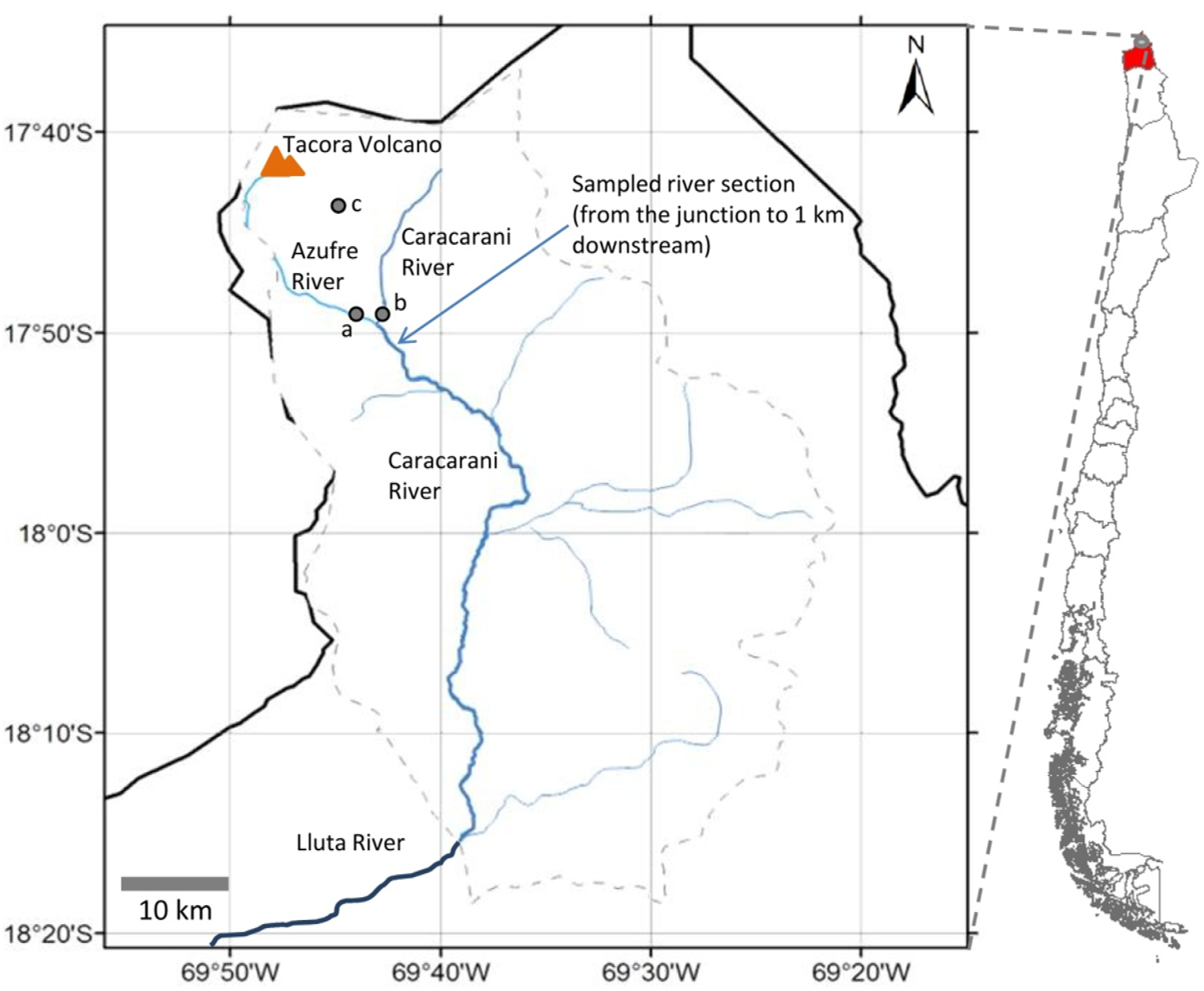
2.1. Site of Study

The Azufre River-Caracarani River confluence is located in the headwater of the upper Lluta River basin, Chile, with an area of 2305 km2 (Figure 1). The confluence is located at 17°50′21′′ S, 69°42′26′′ W and at an elevation of 3986 m. The Azufre River joins the Caracarani River, and from this point downstream it keeps the name of Caracarani River. The Azufre River (“Sulfur River” in English) originates at the Tacora Volcano, near an abandoned sulfur mine and tailings site. The oxidation of sulfur tailings and volcanic geothermal springs produce an acidic stream of high electric conductivity (or EC > 9 mS·cm−1), low pH (pH < 2), and trace elements [15]. In contrast, the pH of the Caracarani River ranges between 8.2 and 8.6, alkalinity ranges between 20 and 232 mg·L−1 of CaCO3, and EC values between 1.2 and 2.2 mS·cm−1. The critical toxic element at this site is arsenic [15]. Water quality data for the Azufre River and Caracarani River are shown in Table 1.
The region of study has a high altitude plateau climate, with negligible precipitation between April and November and a wet season between December and March. As an example, Figure 2 shows the monthly rainfall measured between 2011 and 2012 in the region at an elevation of 3900 m, with 484 mm of precipitation (rain) between November and April. Below zero ambient temperatures occur due to the high altitude and closeness to the Andes [31] and can reach down to −10 °C or lower from May to September, as indicated in Figure 2. High flow rates are driven by increased rainfall during the Bolivian winter, whereas much lower flow rates take place between April and November, as reported in other studies [32,33,34] and reflected in our records from 2010 to 2011 (Figure 3).
The Azufre River-Caracarani River confluence is a remote site. It is located 2200 km from Santiago (Chile’s capital) and 140 km from Arica (the closest main city). Due to the remoteness of the location, extreme weather conditions, and safety protocols, manual sampling and operator-dependent measurements were taken only during the daytime (9 a.m.–5 p.m.). Such constraints did not compromise pursuing the objectives of the study. Continuous measurements of flowrate, temperature, and electric conductivity were performed with data-logging sensors deployed in situ (described below).

2.2. Hydrologic Measurements

The rainfall and ambient temperature were recorded every 15 min by the meteorological station located 8.5 km from the confluence at an elevation of approximately 3900 m (Figure 1). The station was equipped with a data logger (Em50 Data Logger, Decagon Devices, Pullman, WA, USA) connected to a temperature sensor (ECH2O sensor, Decagon Devices, Pullman, WA, USA) and a rain gauge (ECRN-50, Decagon Devices, Pullman, WA, USA).
Water pressure, water temperature, and EC were recorded hourly at the Azufre River and Caracarani River using a data logger (Aqua TROLL 200 Data Logger, InSitu Inc., Bingen, WA, USA). The data presented corresponded to records from January to November 2011. The sensors were installed 700 m upstream of the confluence at the Azufre River and 100 m upstream at the Caracarani River (points a and b in Figure 1, respectively). Conductivity sensors were calibrated with a KCl solution 0.01 M and 1.41 mS·cm−1 at the Caracarani River, and a KCl solution 0.1 M and 12.8 mS·cm−1 at the Azufre River through several field campaigns. Water pressure values in both rivers were corrected using atmospheric pressure values recorded with a barometric sensor (Baro Troll Data Logger, InSitu Inc., Bingen, WA, USA) and utilized to further calculate water depth and estimate stream flow rates through rating curves [35]. These curves were computed after several field campaigns between September 2010 and March 2013, which allowed for obtaining eight points of the rating curve for the Azufre River and four points for the Caracarani River. Stream flow velocity (ms−1) and cross section area (m2) were measured using a handheld acoustic Doppler velocimeter (Flowtracker Handheld ADV, Sontek, San Diego, CA, USA) equipped with an interface to estimate stream flow rate (m3·s−1). Finally, analytical expressions were fitted to these curves in order to automate the estimation of the flow rates from the measured water levels.

2.3. Hydrochemical Measurements and Sampling

Turbidity and pH were measured hourly from 9 a.m. to 5 p.m. during a field campaign in August 2012 at points a and b and at the stream segment downstream of the confluence indicated in Figure 1 (from the confluence to 1 km downstream). Downstream measurements were done at 90, 180, 320, and 1000 m from the junction. A Portable Turbidity Meter (HI 98713, Hanna Instruments, USA) was used and calibrated daily with standardized solutions (0.1 NTU, 1 NTU, 10 NTU, and 100 NTU). The pH and conductivity were measured with a multi-parameter probe (Hach HQ40d portable meter, Hach Company, Loveland, CO, USA). The calibration of the pH sensor was performed using buffer solutions of pH 4, 7, and 10 (Hach Company, Loveland, CO, USA). Correct functioning of the pH electrode at pH < 4 were corroborated by plotting pH measurements against potential measurements (mV) as done by Nordstrom et al. [36].
Turbidity was selected as an in situ proxy measurement for particle formation [37,38]. Field measurements at the site between 2008 and 2012 showed that the concentration of suspended solids larger than 0.45 μm (y value) ranged between 1 and 43 mg·L−1, and were significantly correlated with turbidity (x value) through a mathematical regression of y = 0.71x − 0.56 (coefficient of determination R2 = 0.72, with a level of significance of α = 5% according to a standard normal distribution two-tailed statistical test) [39].
Suspended solids were sampled through several field campaigns (see Table 2). These were collected by using a portable barrel filter of 2 L capacity (Barrel Filter Holder, Geotech Environmental Equipment Inc., Denver, CO, USA). Suspended solids were retained onto pre-weighed cellulose acetate membranes (>0.45 µm from the same company). Aqueous samples (non-filtered samples) were collected in the field, then filtered and stored at 4 °C when conditions allowed.

2.4. Analytical Methods

Membranes containing suspended solids were dried at 40 °C for 24 h and then placed inside Teflon tubes along with 12 mL of aqua regia (HCl and HNO3) for microwave digestion (Mars Microwave System, MarsXpress-5, CEM Corporation, Matthews, NC, USA), according to the EPA protocol number 3015A [40]. Blank membranes were also digested for quality control.
Digested aqueous and solid field samples were analyzed for iron, aluminum, and arsenic through Inductively Coupled Plasma-Optical Emission Spectrometry (ICP-OES, Optima 7300 V, Perkin Elmer, USA).

3. Results and Discussion

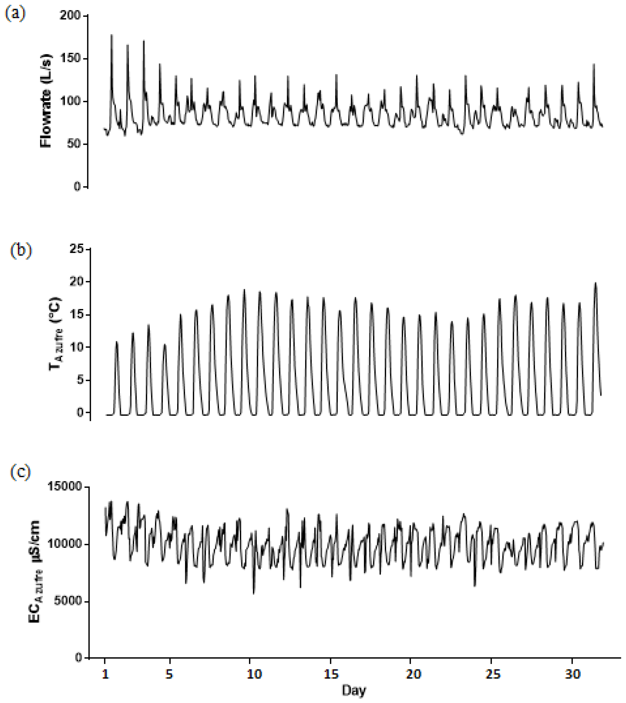
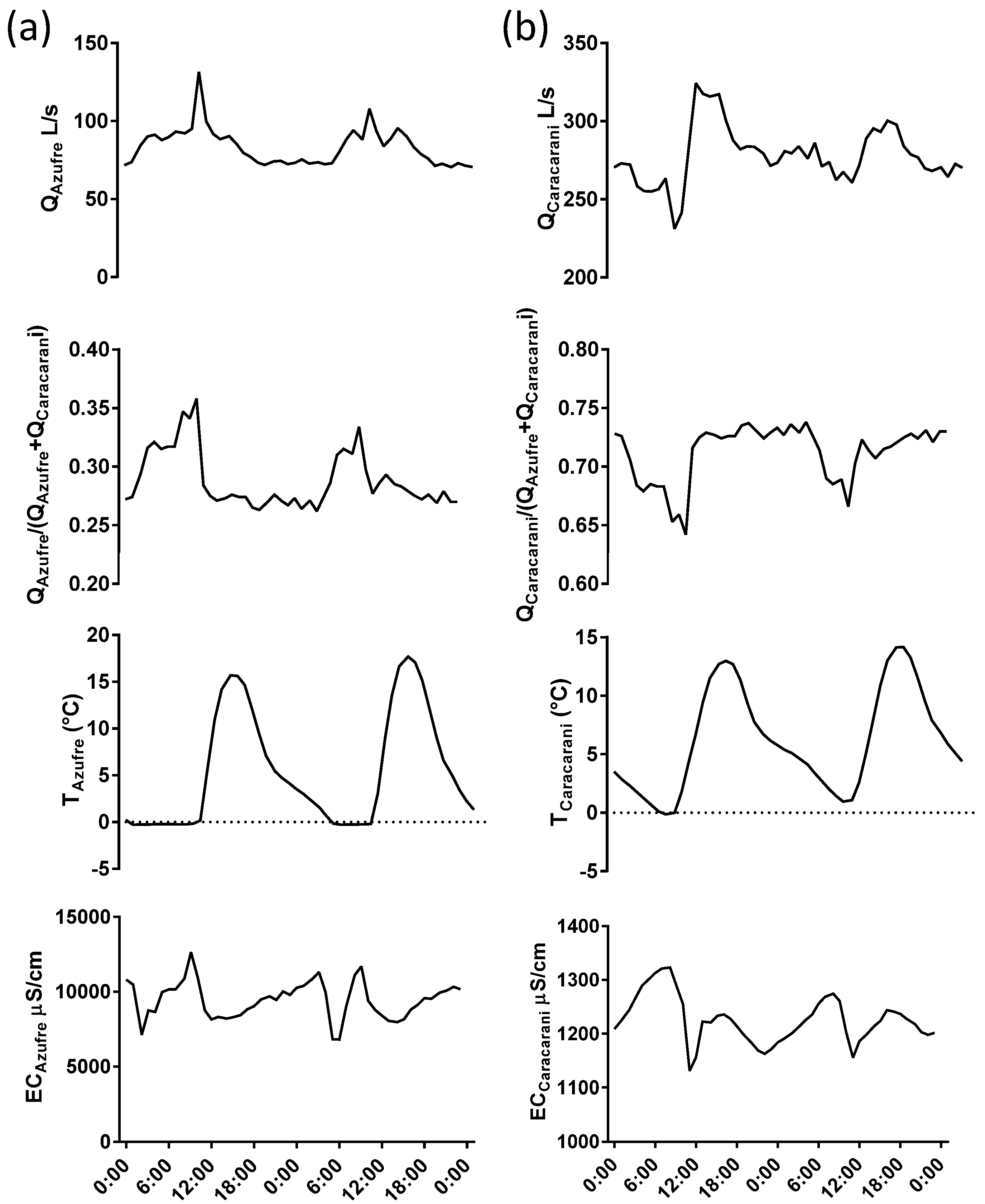
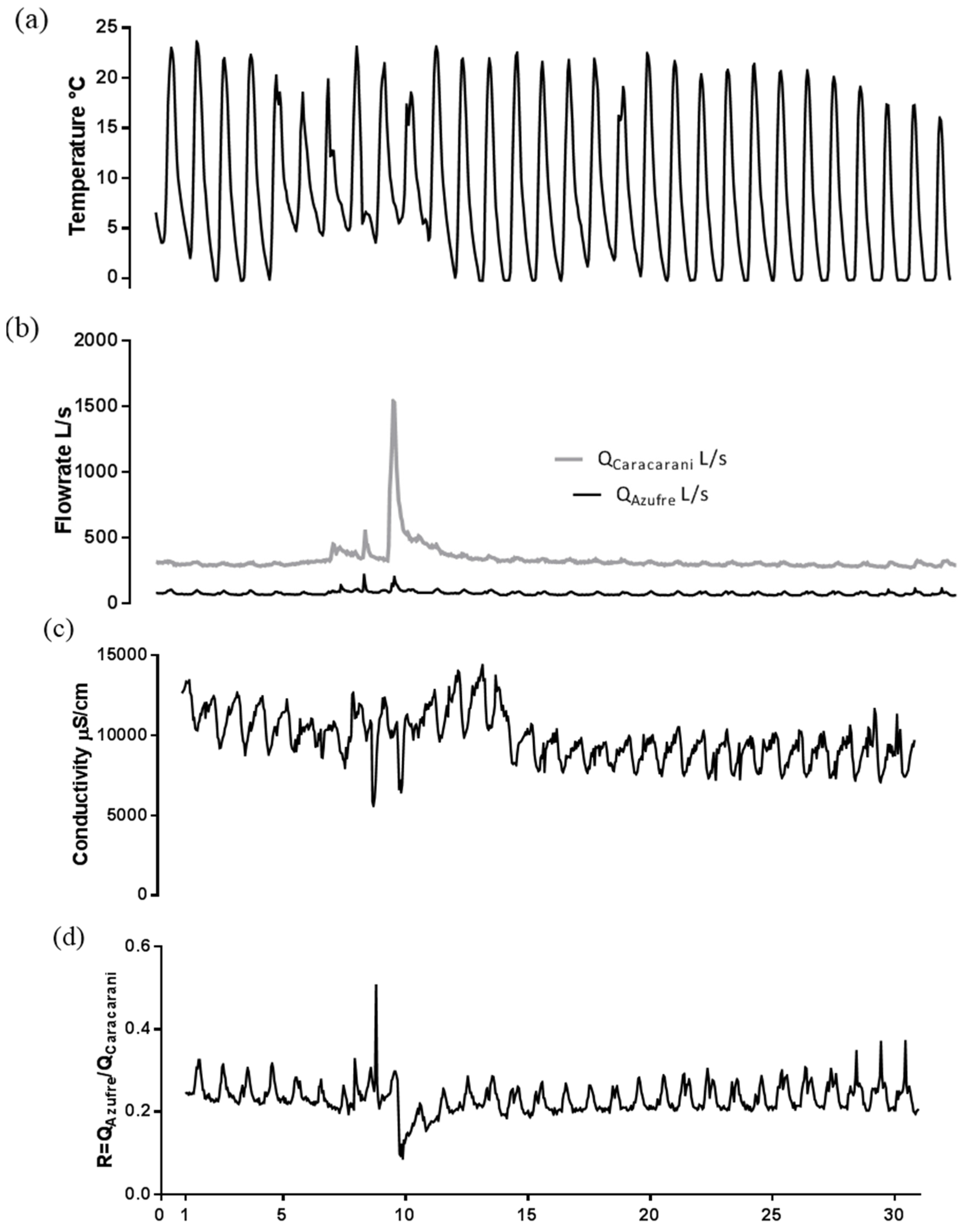
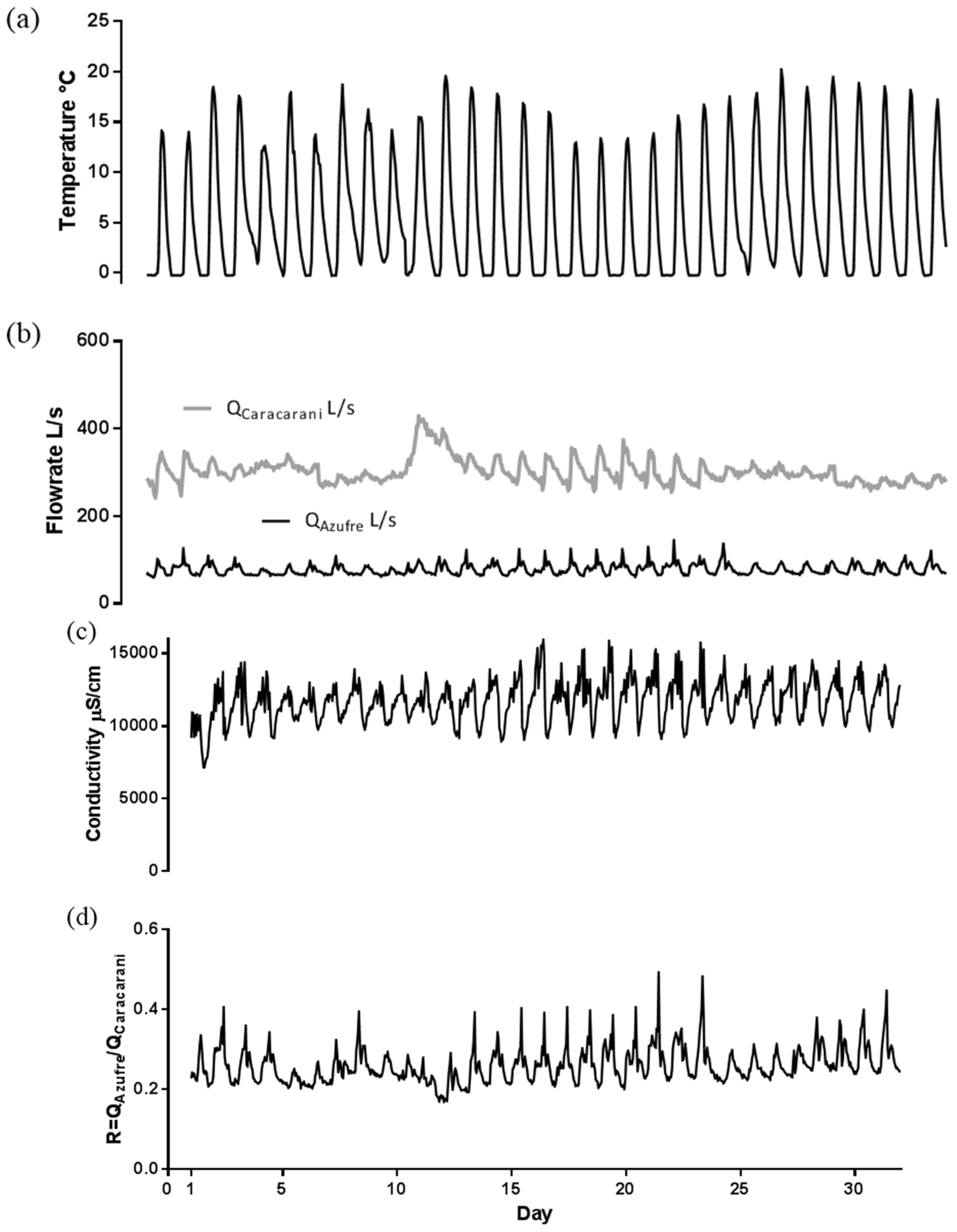
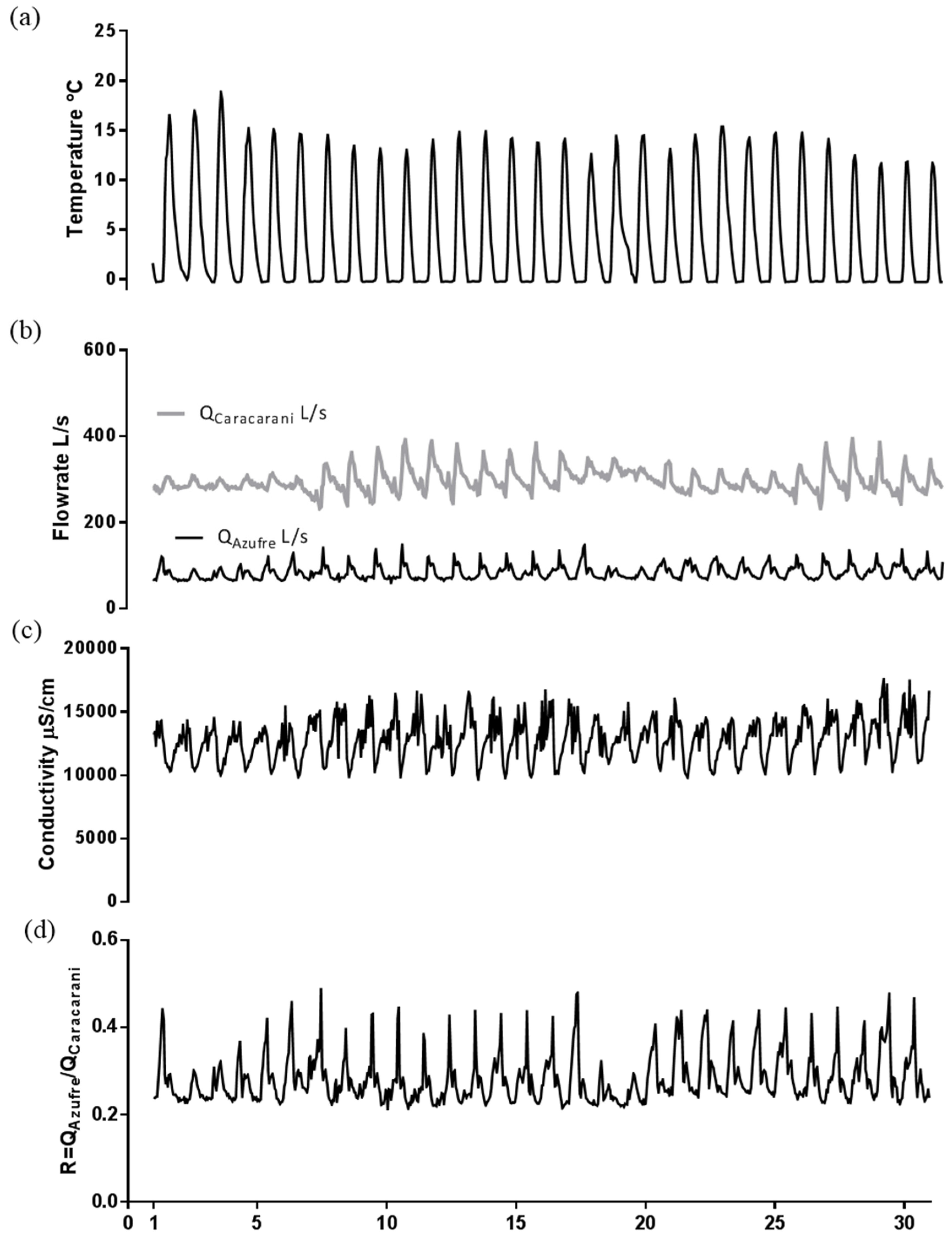
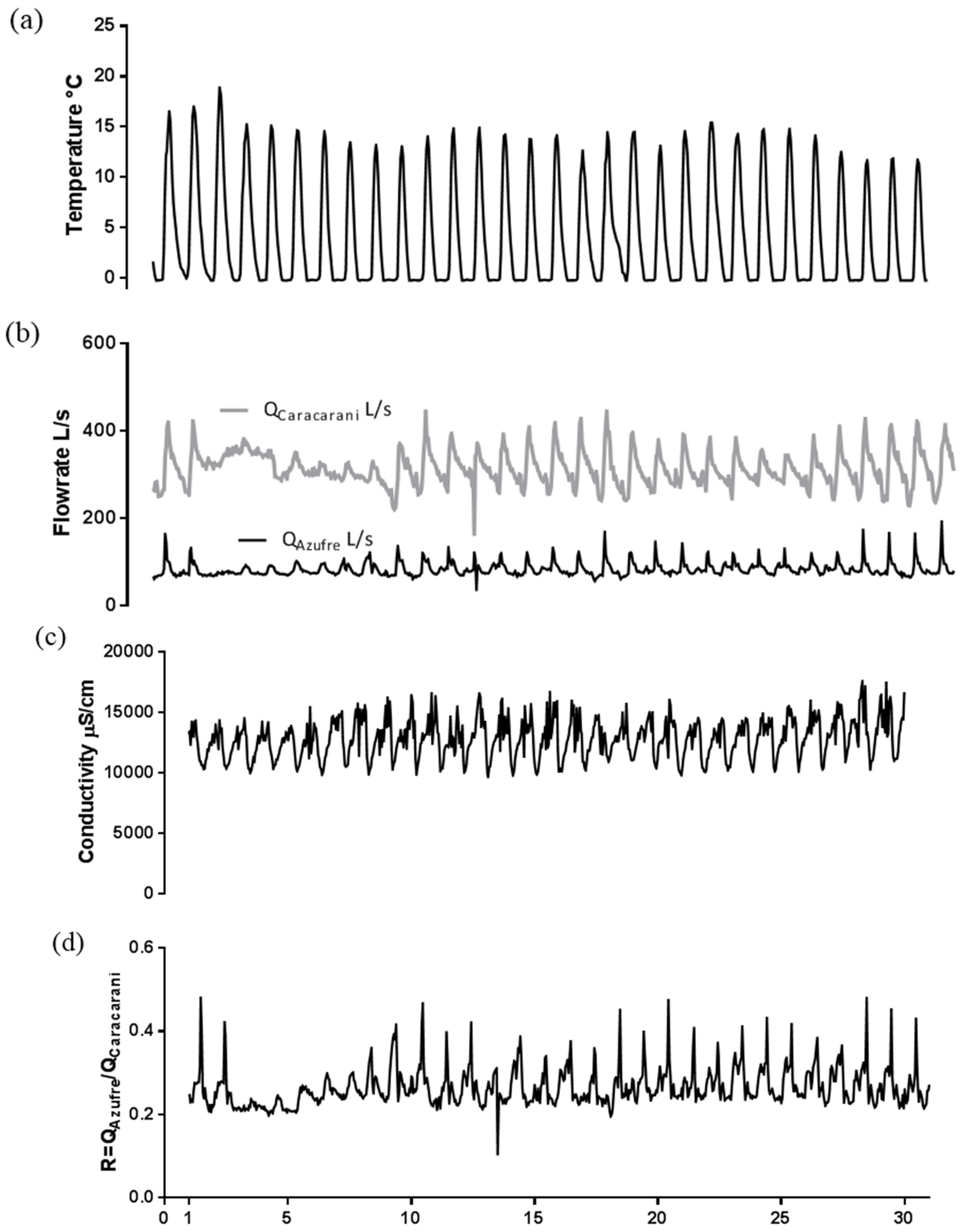
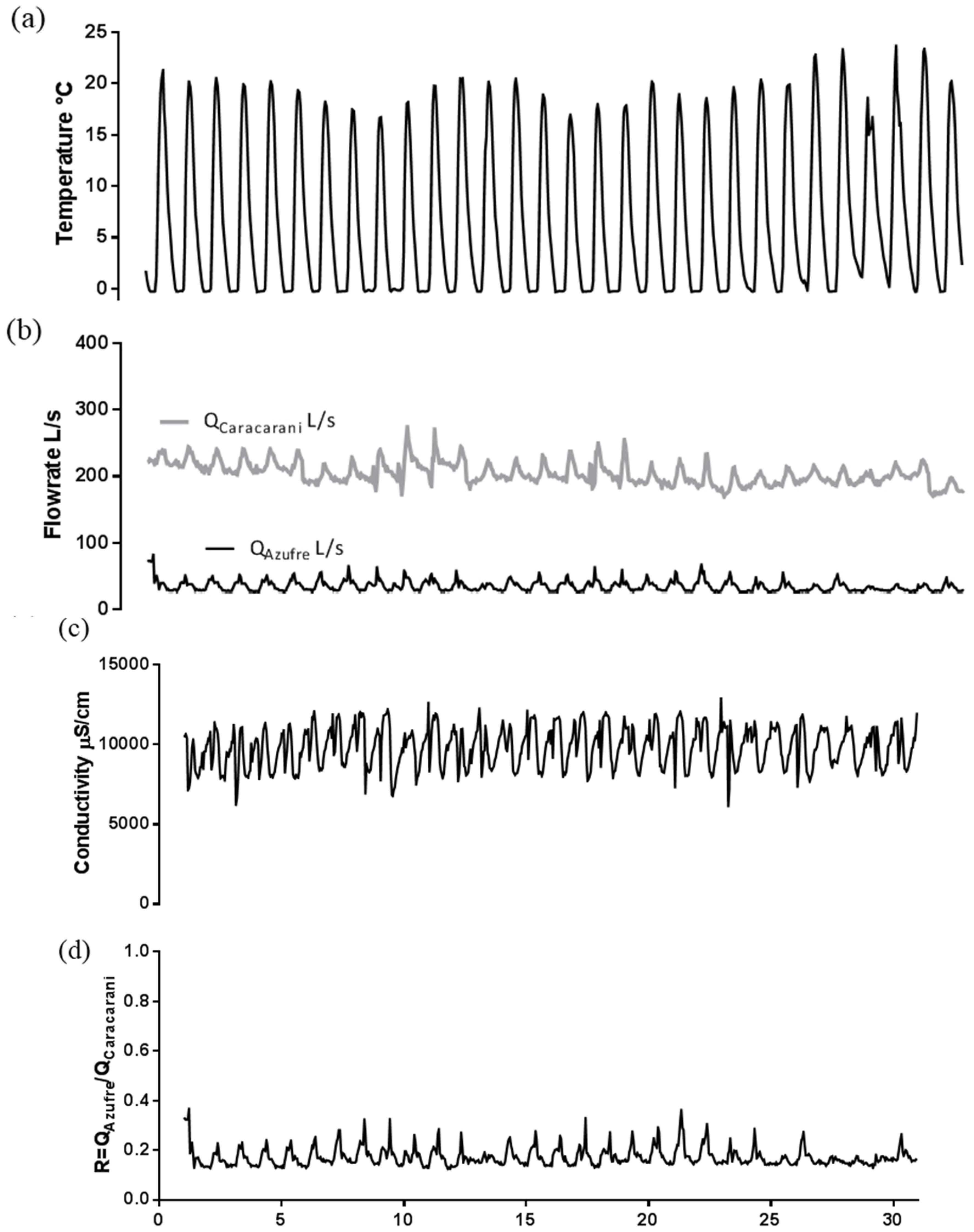
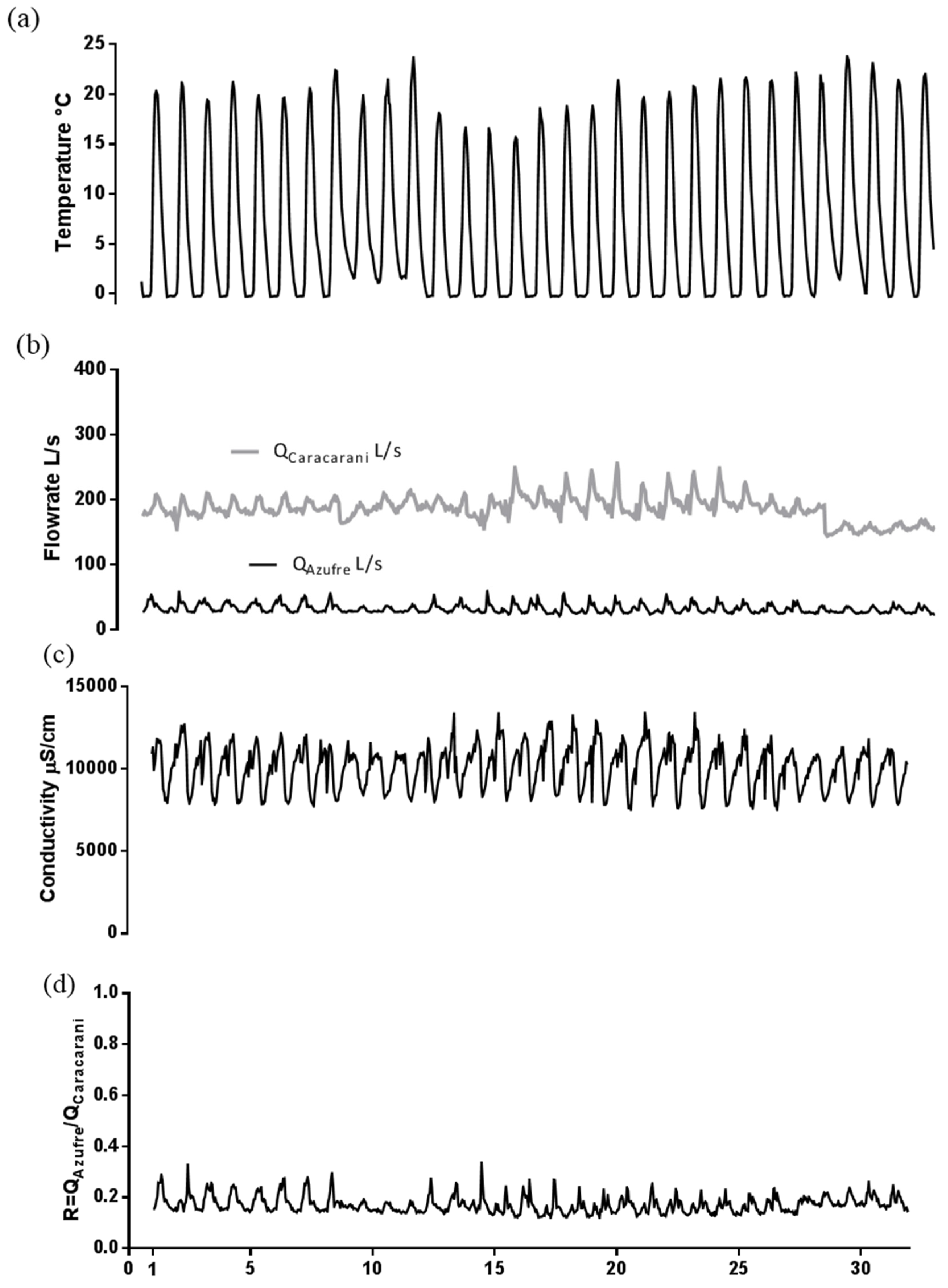
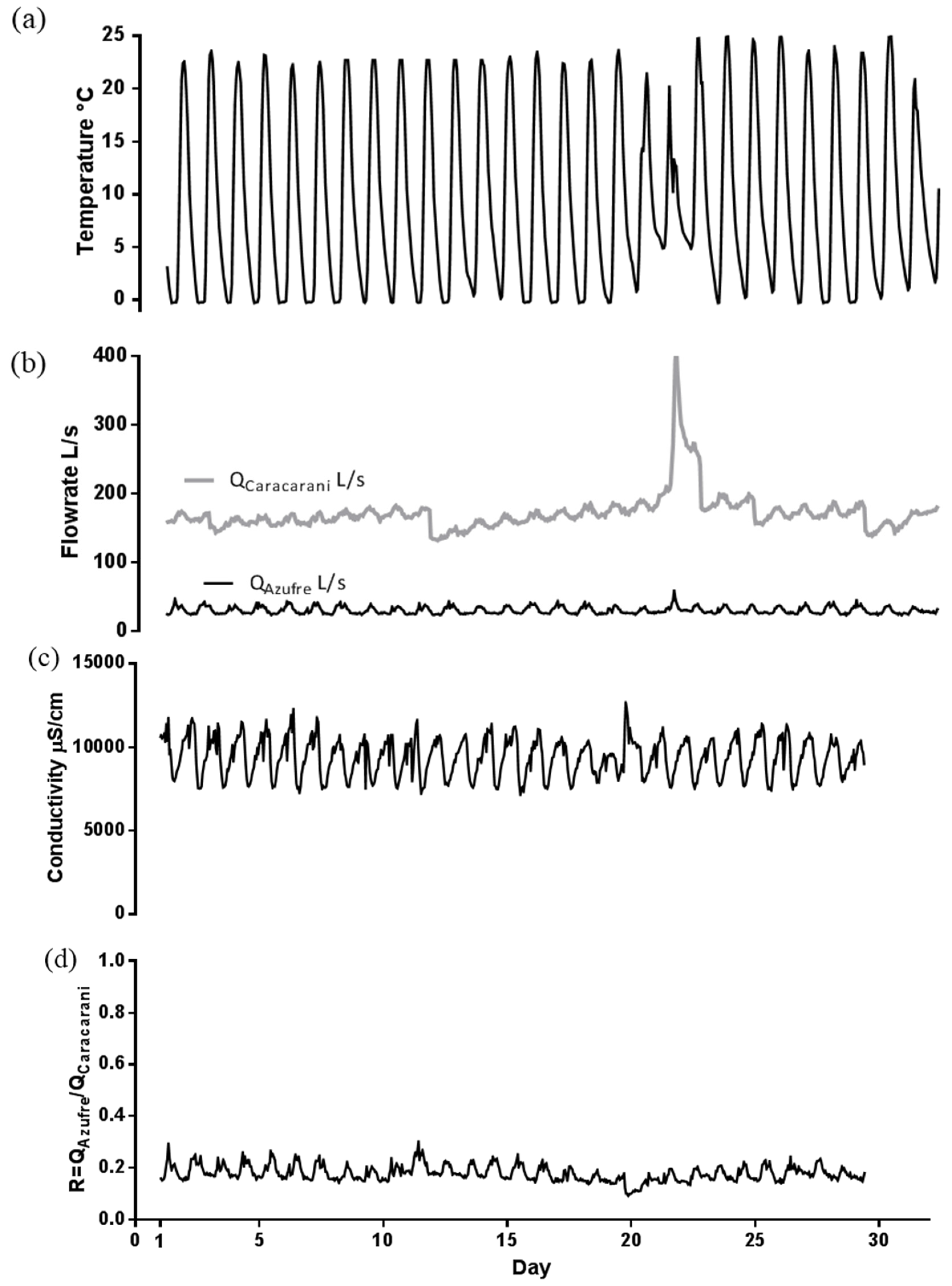
3.1. Diurnal Cycles in Stream Flow Rates, Temperature, and Electric Conductivity

The flow rates of the Azufre River (QAzufre) and Caracarani River (QCaracarani) showed daily cycles, as illustrated in Figure 4, where flow rates measured in August 2011 are shown (additional data is presented in the Supplementary Materials). The periodicity of the time series was identified visually and by means of the autocorrelation function, which determines how the variable x measured at time t correlates with the measured value at time t-k, where k = 1,2,…n is the so called “lag-time” [40]. This test was performed using the Signal Processing Toolbox of Matlab. A strong 24 h periodicity for QAzufre and QCaracarani was found, as well as for the temperature and the EC of the Azufre River (TAzufre and ECAzufre, respectively). As a consequence, the proportion of QAzufre, defined as QAzufre/(QAzufre + QCaracarani)), exhibited the same periodicity.
Daily cycles experienced by QAzufre were attributed to the freezing and thawing of the stream. The Azufre River typically remains at 0 °C from 9 p.m. to 10 a.m. the next morning when the ambient temperatures are negative and can reach down to −13 °C during the colder months (Figure 2). The partial freezing of the Azufre River upstream causes the stream flow rate to drop while the water temperature remains at 0 °C. Once the temperature passes the 0 °C threshold, the melting causes a sudden peak of QAzufre. This process occurred on a daily basis while the ambient temperature was low enough for the stream to remain partially frozen (Figure 4). ECAzufre also exhibited cyclic behavior. This process does not occur between December and April, when stream freezing does not take place and rainfall drives stream flows (see Supplementary Materials).
A temporal cross-correlation analysis (i.e., a lagged correlation analysis between two time series shifted in time relative to one another) [41] was used to detect the correlation between QAzufre and TAzufre data, and between TAzufre and ECAzufre data, which also experience cyclic behavior (data based on the whole 2010–2011 record). Results show that TAzufre and QAzufre correlated (r = 0.38) with a lag time of 7 h, (i.e., QAzufre reaches its maximum value around 7 h after TAzufre reaches its maximum value, see Figure 5). Similarly, a cross correlation was observed between TAzufre and ECAzufre (r = −0.63) with a lag time of 1 h (i.e., ECAzufre reached its minimum value around 1 h after after TAzufre reaches its minimum value). Note that higher values of r were not reached because the water temperature is constrained in the low range to 0 °C, and thus the variability of TAzufre is more limited than that of QAzufre and ECAzufre. However, a standard normal distribution two-tailed statistical test indicated both cross-correlations were statistically significant for a level of significance of α = 5%. Overall, the temporal crossed correlations between these variables further demonstrate that QAzufre was controlled by the freeze–thaw cycles.
The partial freezing of the Caracarani River upstream of the confluence occurs to a lesser extent than for the Azufre River (see Figure 4 and Figure 5). Maximum QCaracarani values occur between noon and 3 p.m., when the temperature of the Caracarani River (TCaracarani) was also at a maximum. These cyclic variations also affect the water quality downstream from the confluence, as the supply of acidity from the Azufre River is counterbalanced by the alkalinity of the Caracarani River (QCaracarani is 2 to 12 times higher than QAzufre).
Maximum stream flowrates at both streams occurred within distinct times of the day. Indeed, 65% of minimum total flow rates in both the Azufre and Caracarani River occurred between midnight and 9 a.m., when both rivers tended to remain partially frozen according to temperature measurements (remained at 0 °C). Seventy-two percent of maximum QAzufre values occurred between 8 a.m. and noon, when the temperature of the Azufre River passed the 0 °C threshold. These variations were coincident with the mixing proportion between the streams (QAzufre/(QAzufre + QCaracarani)) (72% of maximum QAzufre/(QAzufre + QCaracarani) values occurred between 8 a.m. and noon). Finally, maximum flow rates in the Caracarani River, as 77% of maximum QCaracarani values occurred between noon and 4 p.m. Variations in the time QCaracarani reached its maximum might be explained by freezing–melting cycles occurring near its origin, with delayed effects due to the distance to the confluence. Maximum values of QCaracarani/(QAzufre + QCaracarani), however, were widely spread (63% of these values occurred between noon and midnight). This was due to decreased flow rates towards the evening.

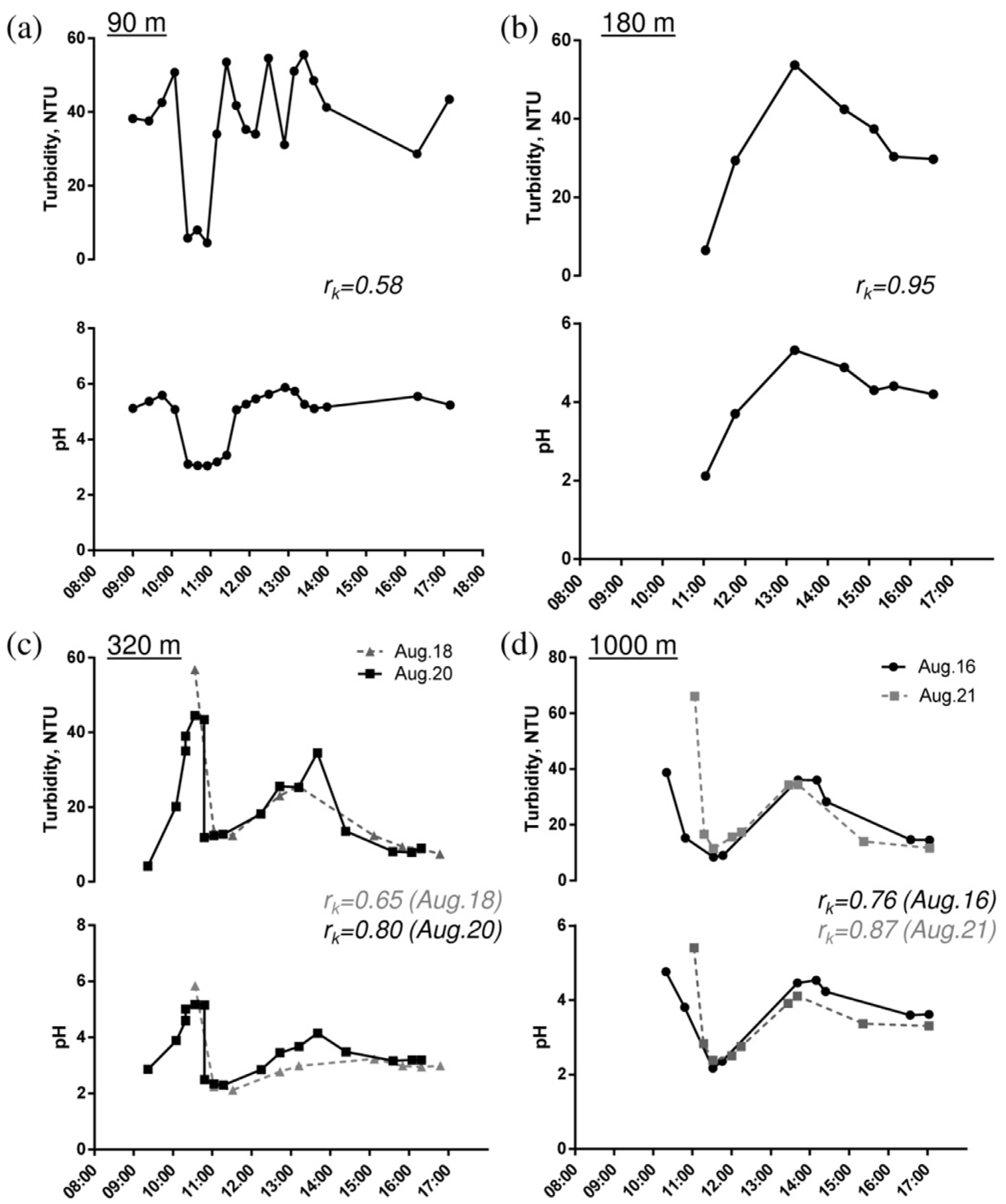
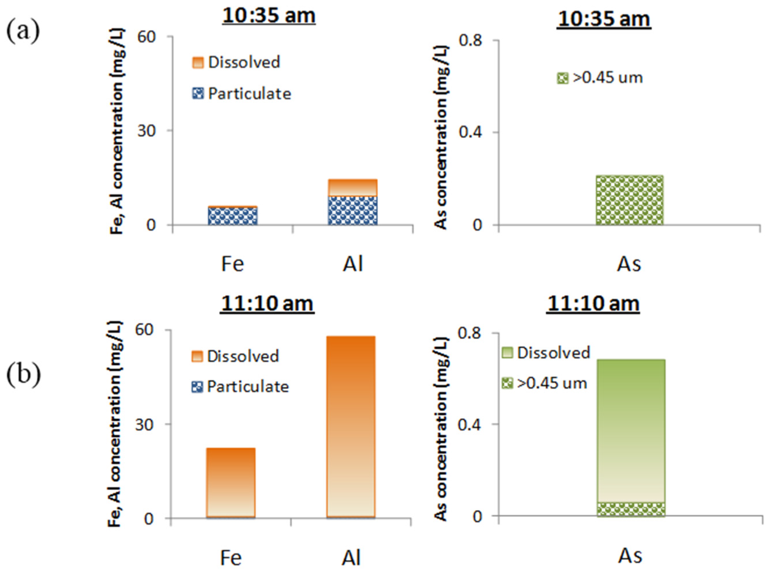
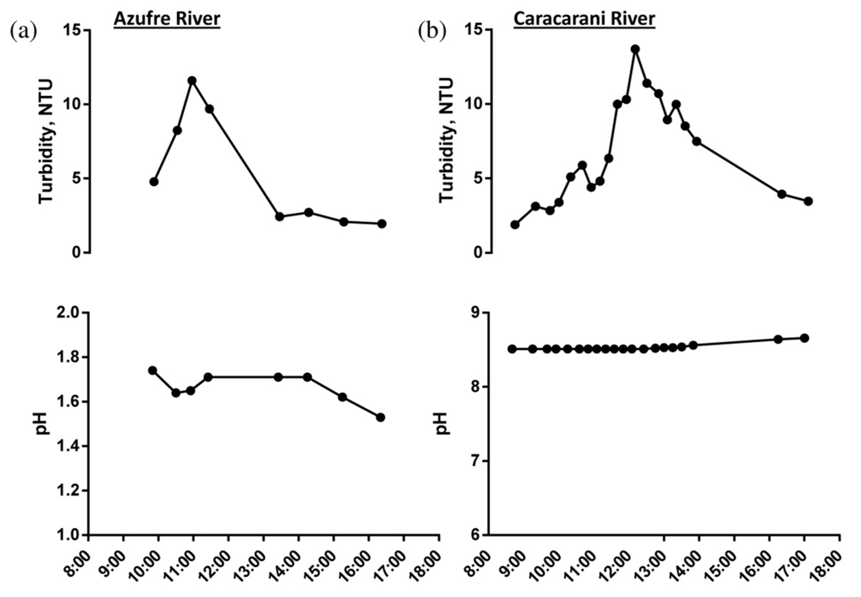
3.2. Diurnal Cycles in Particle Formation Downstream from the Confluence

Diurnal cycles in the formation of suspended solids (detected as changes in turbidity) were also detected downstream from the confluence. Characteristic peaks and drops in turbidity and pH were observed within specific time frames (Figure 6). Global turbidity and pH peaks were consistently observed early in the morning. For example, temporal measurements taken on 20 August at 320 m downstream from the confluence showed a characteristic global turbidity and pH peaks early in the morning (reaching up to 45 NTU at pH 5.2); these peaks were not as clear in the other time series as measurements taken later in the morning. A sudden turbidity and pH drop was consistently observed between 9 and 11 a.m. at all post-confluence sampling points. Another turbidity and pH peak occurred in the afternoon (between noon and 2 p.m.). The consistent peaks in these parameters indicate hourly water quality changes, consistent with the hourly hydrologic changes, as observed in Figure 7. Minimum values of pH and turbidity occurring within the same period maximum values of QAzufre/(QAzufre + QCaracarani) were observed. Local peaks in turbidity and pH occurring within the same period values of maximum QCaracarani were observed.
A high correspondence between turbidity and pH was identified downstream from the confluence. This dependence was determined by pH controlled by incoming inflow ratios (QAzufre/(QCaracarani + QAzufre)), which caused the precipitation of mineral phases attributable to iron and aluminum oxides. Simultaneous measurements of pH and turbidity were significantly correlated, with correlation coefficients (rk) that ranged between 0.58 and 0.95 (see Figure 7). Additionally, turbidity versus pH showed a positive linear regression from pH 2 to approximately 5, as seen in Figure 8. Turbidity (suspended solids) was controlled by the precipitation of iron and aluminum phases, which are pH-controlled chemical reactions. Evidence of this is the presence of suspended solids, collected in the field, which showed high concentrations of iron and aluminum (Table 2). Furthermore, we developed a preliminary geochemical model that considered the formation of amorphous iron hydroxide (Fe(OH)3(a)) and amorphous aluminum hydroxide (Al(OH)3(a)) at different mixing ratios between the Azufre River and Caracarani River (see Supplementary Materials). This simplified model showed that Fe(OH)3 was feasible at pH > 3, while Al(OH)3 was feasible at pH > 5. It is also known that in natural systems Fe(OH)3(a) becomes saturated at pH > 3 and that aluminum hydroxide precipitates at pH > 4.5 [42]. Although there are other iron and aluminum phases involved (such as hydrosulfates [43]), the analysis is consistent with how turbidity simultaneously increases with pH. These increases in turbidity downstream are not caused by incoming of suspended solids from upstream of the confluence. The turbidity measured at the Azufre River and Caracarani River fluctuated between 2 and 14 NTU, respectively. One hundred percent of turbidity values measured downstream were higher than 4 NTU (69% were higher than 14 NTU), indicating that turbidity increases were mainly due to pH-dependent chemical reactions.
The peaks of pH occurring before noon can be attributed to lower total flow rates, which triggered higher turbidity values (no particular patterns in QAzufre/(QAzufre + QCaracarani) were found). Additionally, lower flowrates (higher residence times [44,45]), caused increases in turbidity. The subsequent drop in pH observed between 9 a.m. and noon (Figure 7) was caused by peaks in QAzufre/(QAzufre + QCaracarani) (Figure 4 and Figure 6), thus diminishing turbidity. Diminished suspended solids can be attributed to dissolved precipitates. Finally, the local peak in pH observed in the afternoon (Figure 7) was coincident with higher values of QCaracarani (Figure 5 and Figure 6). Despite the fact that the alkalinity of the Caracarani River was moderate (20–232 mg CaCO3·L−1, see Table 1), its discharge contributed to increase pH, thus an increase in turbidity. Overall, our results indicate that diurnal flow rate behavior controlled downstream pH. Downstream pH triggers the precipitation of iron and aluminum mineral phases at streams affected by acid drainage [42,43,46]. In consequence, diurnal cycles in the formation of iron and aluminum phases, known to control the cycling of arsenic in the environment [23,42,43,46,47,48], also constitute an important factor in the fate and transport of this toxic element.

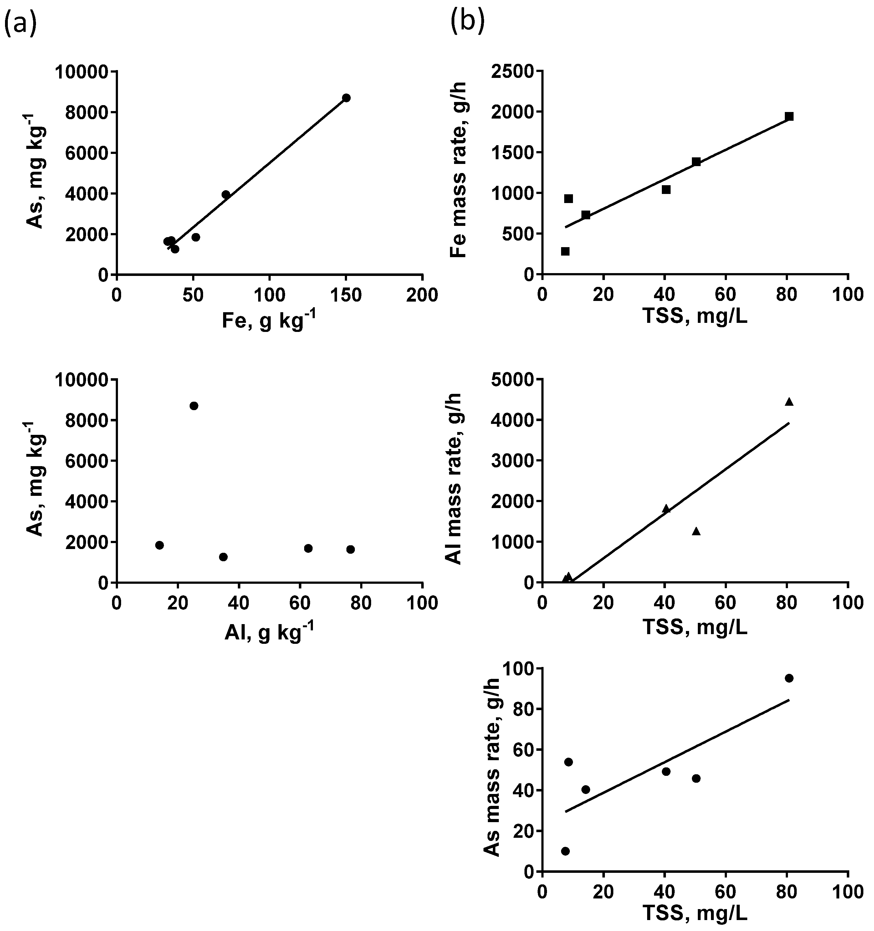
3.3. The Fate and Transport of Metals Controlled by Freeze–Thaw Cycles

The effect diurnal changes in pH due to incoming flow ratios have on the fate of iron, aluminum, and arsenic can be visualized by comparing analyses of samples taken before and after the thawing of the Azufre River (Figure 9). A sample taken at 10:35 a.m. indicated a pH value of 5.2 and turbidity value of 45 NTU, dropping to pH 2.3 and turbidity of 13 NTU at 11:10 a.m. Total concentrations of iron, aluminum, and arsenic were considerably lower at 10:35 a.m. than those measured at 11:10 a.m. (5.4 vs. 22.2 mg·L−1 of total Fe, 14.7 vs. 58.5 mg·L−1 of total Al, and 0.18 vs. 0.63 mg·L−1 of As). Moreover, particulate fractions were much higher when higher pH values were measured, as shown in Figure 9. The abrupt increase in metal concentrations occurred within the same time range when the higher inflow of the Azufre River was observed. The sudden inflow of the Azufre River was not only higher in flow rate, but also carried higher concentrations of chemical species, explaining the higher concentration of iron, aluminum, and arsenic. This explains why higher total flux occurred within a matter of minutes in a pulse-like manner. Additionally, low pH promotes the dissolution of iron and aluminum mineral phases (iron and aluminum hydroxides), increasing concentration of dissolved metals, a condition that does not favor arsenic sorption [47,48]. This comparison of samples, taken with only an hour from each other, showed that important changes in water quality are caused by diurnal variations in stream flow rate, particularly due to freeze and thaw cycles.
The mass rate of elements depends on both the concentration of total suspended solids (TSS) and the concentration of metals. This was determined by estimating the rate of iron, aluminum, and arsenic in g h−1, as follows:
Mass rate of elements, g·h−1 = [TSS, mg·L−1] × [Metal, mg·kg−1] × Q, L·h−1 × 10⁻⁹ mg·kg−1,
where TSS: concentration of total suspended solids, Element: concentration of the element (Fe, Al or As); Q: stream flowrate of the Caracarani River downstream from the confluence.
Indeed, arsenic reached its maximum concentration in the solid phase at pH 3.8 (Table 2); however, the observed concentration of total suspended solids was only 9 mg/L. The highest concentration of suspended solids (81 mg/L) occurred at pH 5.9. Results showed that the mass rate of arsenic, iron, and aluminum in the solid phase, at a constant flowrate of 200 L·s−1, increased with a higher concentration of suspended solids, as shown in Figure 10. This means that the higher the concentration of total suspended solids, the higher the mass rate of elements in solid phase will be. Values of particulate and dissolved fractions of arsenic downstream from the Azufre River-Caracarani River confluence were presented in Guerra et al. [39]. Particulate arsenic concentration ranged between 75% and 95% within a wide range of pH values (pH 3 to 7); there was no increase or decrease of particulate arsenic concentration with increasing pH. This indicates that particulate arsenic transport, in g·h−1, was controlled by the concentration of total suspended solids, which is a result of the pH of the stream. Immobilization of arsenic is promoted through the precipitation of mineral phases, reflected in the increased concentration of suspended solids. This is favorable in terms of site remediation: when iron and aluminum are part of the solid phase, these have the potential to settle on the stream bed. As arsenic sorption occurs, this metalloid will also be immobilized. Additionally, arsenic and iron were highly correlated (Figure 10), reaffirming the role of iron phases downstream from the confluence. A controlling factor in the fate of arsenic is the sorption or co-precipitation onto freshly precipitated iron and aluminum mineral phases (hydroxides and hydrosulfates) [42,45]. In the case of the Azufre River–Caracarani River confluence, diurnal changes in flowrate (in consequence, in the proportion QAzufre/(QAzufre + QCaracarani) control downstream pH. pH triggers reactions of precipitation of iron and aluminum phases. In consequence, particulate arsenic (sorbed or co-precipitated onto mineral phases) is also prone to experience diurnal cycles. During the hours when QAzufre is at peak values, iron hydroxides are dissolved, and, as a consequence, arsenic is again released into the aqueous phase. For this reason, the estimation of the mass rate of elements in solid phase (g·h−1) is relevant, in order to determine at which moments of the day arsenic transport is promoted.
An integration of the hydrologic and chemical processes that were described can be presented through a conceptual model, as shown in Figure 11. When QAzufre/(QAzufre + QCaracarani) is high, pH is low and, as a consequence, so is the concentration of total suspended solids (surrogate for iron and aluminum mineral phases). At a low pH, total arsenic is high (Figure 9) and the low availability of solid phases indicates that the particulate arsenic mass rate is low (thus, dissolved arsenic will be high). When QAzufre/(QAzufre + QCaracarani) is lower, pH is higher and, as a consequence, the formation of mineral phases is promoted. At higher pH values, total arsenic is lower (Figure 9), and the higher availability of mineral phases promotes arsenic sorption. This indicates that the particulate arsenic mass rate is higher at these conditions.
This study shows how cycles in flow rate, due to daily freeze-thaw processes, can also constitute a controlling factor in the fate and transport of toxic elements downstream a confluence affected by acid drainage. It is also necessary to consider these freeze-thaw processes and their effect in arsenic transport at distances further downstream the confluence. Modeling of arsenic-rich sediments at a future reservoir located downstream, at the Lluta Valley, showed the potential desorption of arsenic from the sediments [49]; the cyclic transport of dissolved or particulate arsenic may also have effects on the chemical dynamics of reservoirs near areas affected by acid drainage.

4. Conclusions

The objective of this paper was to show how daily variations in stream flow rates due to freeze and thaw cycles control metals’ transport downstream in streams affected by acid drainage. We characterized the hydrologic and geochemical behavior of the Azufre River (pH < 2) and Caracarani River (pH ~8.6) confluence (northern Chile) by measuring stream flow rates, temperature, electric conductivity, pH, and turbidity and analyzing the concentration of metals in the aqueous phase. We showed how cyclic hydrological variations control the fate of contaminants in a watershed affected by acid drainage. Coincidental diurnal patterns were observed between flow rates, turbidity, and pH. Important drops in pH occurred when peaks in QAzufre (QAzufre/(QAzufre + QCaracarani)) occurred, with consequential drops in turbidity. Similarly, peaks in pH occurred within the same time range when the maximum QCaracarani occurred, with consequential drops in turbidity. Changes in the flow rate of the Azufre River were caused by freeze and thaw cycles. The conclusions of this work are as follows:
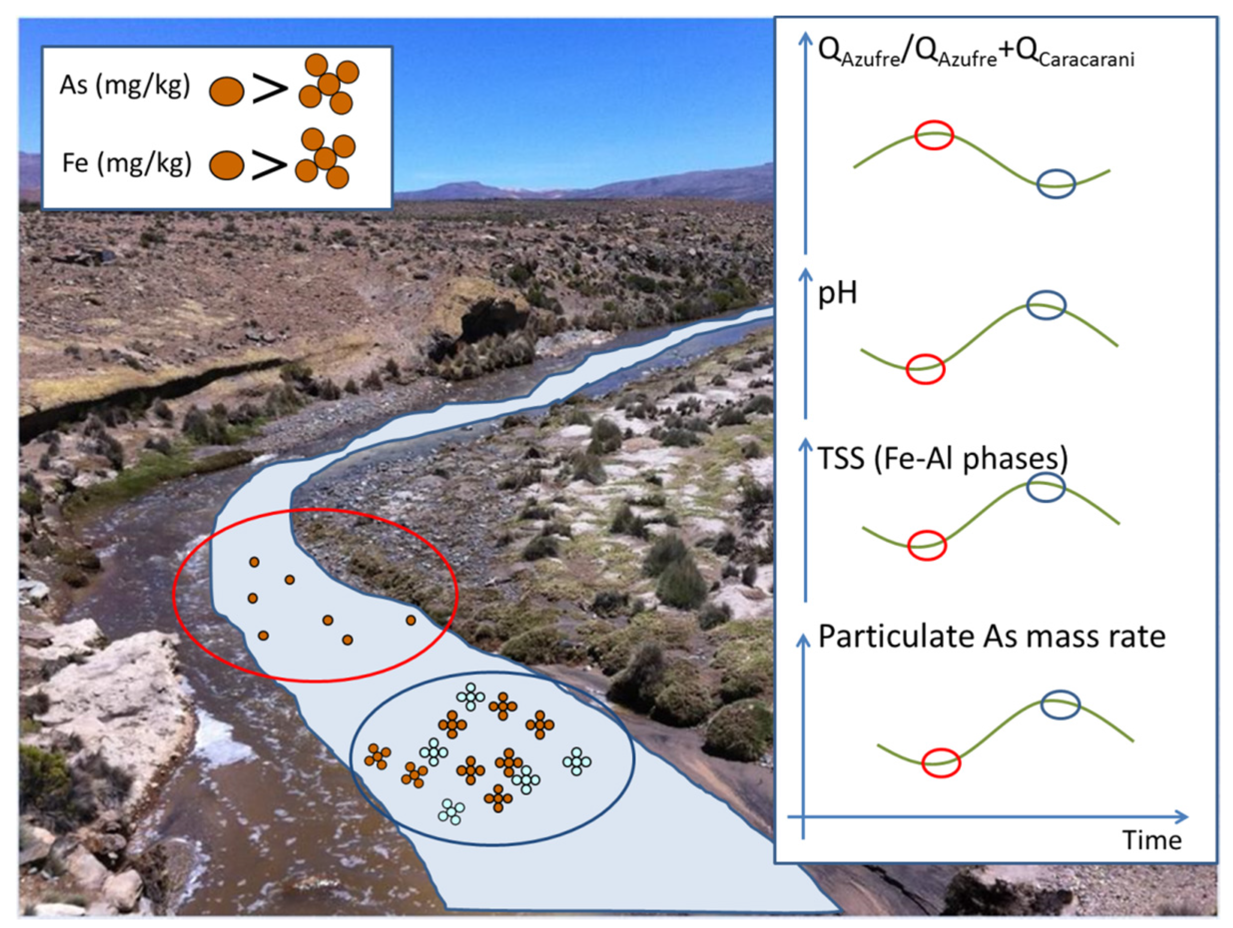
  • Due to the below-zero temperatures reached at night, QAzufre was controlled by daily freeze–thaw processes. The daily pulse in flow rate in the acid drainage results in a pulse in the flux of dissolved metals downstream and in the dissolution of suspended solids. Although this process occurred for only a few minutes every day, it was sufficient to mobilize metals and degrade water quality downstream due to, for example, higher flux of dissolved arsenic.
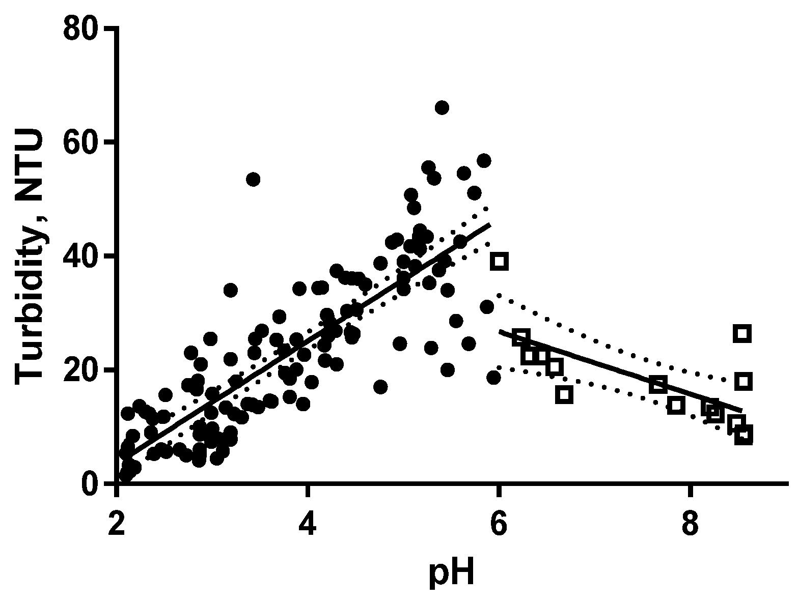
  • Diurnal behavior of water quality downstream from the confluence was controlled by diurnal changes in the upstream flow regime. Clear patterns in pH occurred concurrently with daily peaks in QAzufre and QCaracarani. As a consequence, turbidity (surrogate for suspended solids formed downstream as a consequence of the precipitation of mineral phases) also experience daily peaks. In this study, hourly variations at a confluence affected by acid drainage due to daily freeze and thaw cycles were identified, showing that drastic changes in water quality are not limited to seasonal factors (i.e., snow melts, increase in rainfall) but could occur within intraday time scales.
  • The formation of mineral phases downstream from the confluence was enhanced at distinct times of the day (dawn and mid-afternoon). Since the formation of suspended solids controlled the fate and transport of metals, attenuation of dissolved contaminants would improve within these time lapses, as particles have the potential to settle onto the streambed.
Hydrologic diurnal cycles constitute an important factor to consider when exploring sites affected by acid drainage. Diurnal cycles in flow rate, particularly in streams affected by acid drainage, caused by freeze and thaw cycles are prone to occur at other sites where below-zero temperatures occur, such as mine sites located at high altitudes. The processes observed at this site impacted on the downstream water quality in a cyclical manner through daily “pulse-type” discharges. These diurnal changes may cause variability in the analysis of freshwater samples, critical in planning sampling and monitoring campaigns in these types of systems. The knowledge of when and where attenuation/mobilization of contaminants occurs is important to prevent toxic elements from reaching points of use for human consumption and agriculture.

Acknowledgments

We thank Marina Coquery and Jean-François Gaillard for their comments on our work. We also thank Alejandra Vega for providing hydrological data. This research was funded by Fondecyt 1130936/2013 and CONICYT-FONDAP 15110020. The CONICYT scholarship (folio number 2110173) is acknowledged by Paula Guerra.

Author Contributions

The manuscript was written by Paula Guerra, but all the authors contributed to its preparation and review. Hydrochemical field data was mainly obtained by Kyle Simonson. Data analyses were carried out by Paula Guerra in discussion with Jorge Gironas and Pablo Pasten.

Conflicts of Interest

The authors declare no conflict of interest.

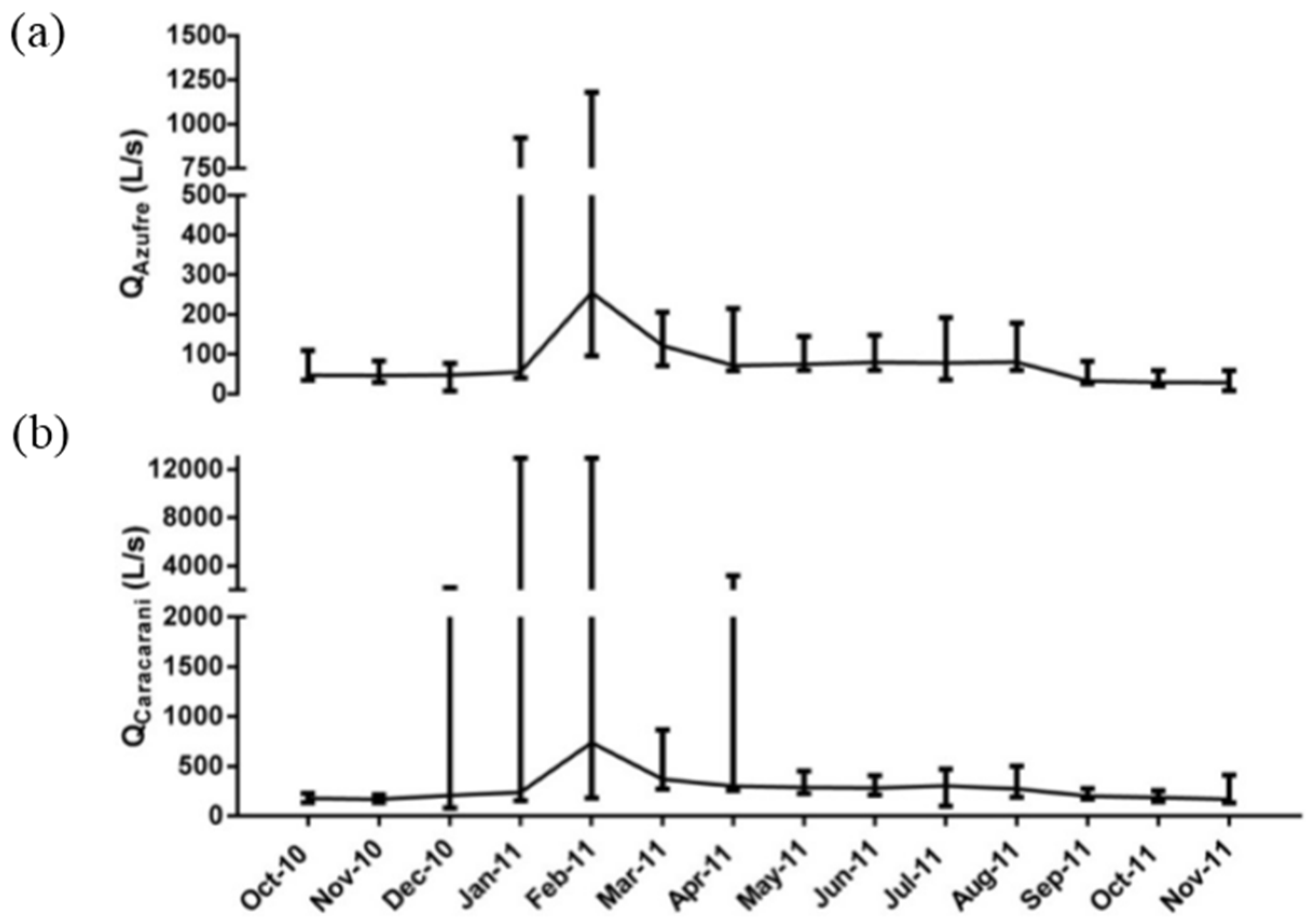
Appendix A: Caracarani River and Azufre River flow rates, Azufre River temperature, Azufre River electric conductivity and mixing ratios arranged per month (January 2011–November 2011).

Figure A1. Hourly hydrological data from January 2011. (a) Azufre River temperature (TAzufre); (b) Azufre River (QAzufre) flow-rates. The axis depicts the days of the month. QAzufre was extrapolated for values greater than 250 L/s.
Water 08 00074 g012
Figure A2. Hourly hydrological data from February 2011. (a) TAzufre; (b) QAzufre. The axis depicts the days of the month. QAzufre was extrapolated for values greater than 250 L/s.
Water 08 00074 g013
Figure A3. Hourly hydrological data from March 2011. (a) TAzufre; (b) QAzufre. The axis depicts the days of the month.
Water 08 00074 g014
Figure A4. Hourly hydrological data from April 2011 (a) TAzufre; (b) QAzufre and QCaracarani; (c) Mixing ratio R; (d) Azufre River electric conductivity (ECAzufre). The axis depicts the days of the month. QCaracarani was extrapolated for values > 350 L/s.
Water 08 00074 g015
Figure A5. Hourly hydrological data from May 2011. (a) TAzufre; (b) QAzufre and QCaracarani; (c) Mixing ratio R; (d) ECAzufre. The axis depicts the days of the month. QCaracarani was extrapolated for values > 350 L/s.
Water 08 00074 g016
Figure A6. Hourly hydrological data from June 2011. (a) TAzufre; (b) QAzufre; and QCaracarani; (c) Mixing ratio R; (d) ECAzufre. The axis depicts the days of the month. QCaracarani was extrapolated for values > 350 L/s.
Water 08 00074 g017
Figure A7. Hourly hydrological data from July 2011. (a) TAzufre; (b) QAzufre and QCaracarani; (c) Mixing ratio R; (d) ECAzufre. The axis depicts the days of the month. QCaracarani was extrapolated for values > 350 L/s.
Water 08 00074 g018
Figure A8. Hourly hydrological data from September 2011. (a) TAzufre; (b) QAzufre and QCaracarani; (c) Mixing ratio R; (d) ECAzufre. The axis depicts the days of the month.
Water 08 00074 g019
Figure A9. Hourly hydrological data from October 2011. (a) TAzufre; (b) QAzufre and QCaracarani; (c) Mixing ratio R; (d) ECAzufre. The axis depicts the days of the month.
Water 08 00074 g020
Figure A10. Hourly data from November 2011. (a) TAzufre; (b) QAzufre and QCaracarani; (c) Mixing ratio R; (d) ECAzufre. The axis depicts the days of the month. QCaracarani was extrapolated for values > 350 L/s.
Water 08 00074 g021

Appendix B: Turbidity and pH data from the Azufre River and Caracarani River (upstream of the confluence).

Figure B1. Daily turbidity and pH time series measured upstream of the confluence at the Azufre River (a) and Caracarani River (b). pH remained relatively constant in both cases, whereas turbidity reached a peak at around 12 p.m. and 11 a.m., respectively.
Water 08 00074 g022

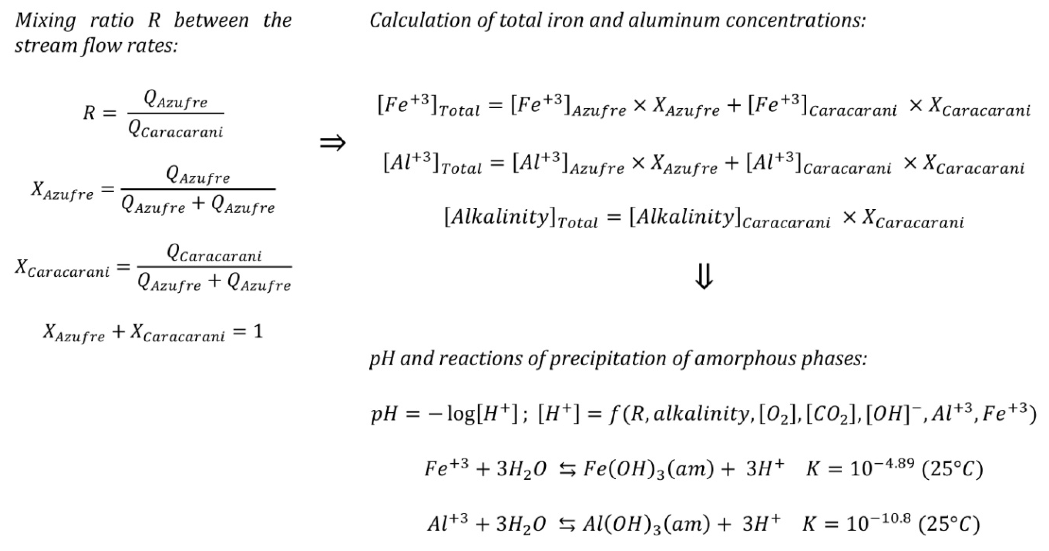
Appendix C: Preliminary geochemical model.

To build a preliminary geochemical model, the main reactions considered were the precipitation of Fe(OH)3(am) and Al(OH)3(a). A chemical equilibrium model for downstream mixing was developed to simulate the formation of these as freshly precipitated phases as a function of the mixing ratio (VAzufre/VCaracarani). The pH was also simulated. The water quality considered for simulations is summarized in Table C1. The calculations were performed using the PHREEQC code (Parkhurst and Appelo, 1999) and wateq4f.dat thermodynamic database (Dzombak and Morel, 1990). Figure C1 describes the geochemical model. Other phases are relevant to systems affected by acid drainage (such as Schwertmannite and Basaluminite) and must be considered further to improve the current model.
Table C1. Representative water quality of the Azufre River and Caracarani River used to simulate the pH concentration of Fe(OH)3(am) + Al(OH)3(am) using the PHREEQC code.
ParameterUnitAzufre RiverCaracarani River
pH -2.28.7
Temperature °C1010
Alkalinity mg CaCO3/L0200
SO4−2 mg/L2450477
Cl mg/L920190
Na+ mg/L333170
K+ mg/L8820
Ca+2 mg/L233120
Mg+2 mg/L15955
Total Fe mg/L490.9
Total Al mg/L1560.7
Total As mg/L2.10.05
Total B mg/L19.73.3
Total Zn mg/L9.80.1
Figure C1. Conceptual model of the precipitation of Fe(OH)3(a) and Al(OH)3(a) as a function of the mixing ratio. pH was estimated as a function of coupled reactions that include precipitation and other acid–base reactions (i.e., carbonate system).
Water 08 00074 g023

References

  1. Aubert, A.H.; Gascuel-Odoux, C.; Merot, P. Annual hysteresis of water quality: A method to analyse the effect of intra- and inter-annual climatic conditions. J. Hydrol. 2013, 478, 29–39. [Google Scholar] [CrossRef]
  2. Davies, T.D.; Tranter, M.; Blackwood, I.L.; Abrahams, P.W. The character and causes of a pronounced snowmelt-induced acidic episodes in a stream in a Scottish subarctic catchment. J. Hydrol. 1993, 146, 267–300. [Google Scholar] [CrossRef]
  3. Davies, T.D.; Tranter, M.; Wigington, P.J., Jr.; Eshleman, K.N. Acidic episodes in surface waters in Europe. J. Hydrol. 1992, 132, 25–69. [Google Scholar] [CrossRef]
  4. Gelfan, A. Extreme snowmelt floods: Frequency assessment and analysis of genesis on the basis of the dynamic-stochastic approach. J. Hydrol. 2010, 388, 85–99. [Google Scholar] [CrossRef]
  5. Iwata, Y.; Nemoto, M.; Hasegawa, S.; Yanai, Y.; Kuwao, K.; Hirota, T. Influence of rain, air temperature, and snow cover on subsequent spring-snowmelt infiltration into thin frozen soil layer in northern Japan. J. Hydrol. 2011, 401, 165–176. [Google Scholar] [CrossRef]
  6. Corriveau, J.; Chambers, P.A.; Yates, A.G.; Culp, J.M. Snowmelt and its role in the hydrologic and nutrient budgets of prairie streams. Water Sci. Technol. 2011, 64, 1590–1596. [Google Scholar] [CrossRef] [PubMed]
  7. Moncur, M.C.; Ptacek, C.J.; Hayashi, M.; Blowes, D.W.; Birks, S.J. Seasonal cycling and mass-loading of dissolved metals and sulfate discharging from an abandoned mine site in northern Canada. Appl. Geochem. 2014, 41, 176–188. [Google Scholar] [CrossRef]
  8. Nimick, D.A.; Gammons, C.H.; Parker, S.R. Diel biogeochemical processes and their effect on the aqueous chemistry of streams: A review. Chem. Geol. 2011, 283, 3–17. [Google Scholar] [CrossRef]
  9. Ryan, R.J.; Packman, A.I. Changes in streambed sediment characteristics and solute transport in the headwaters of Valley Creek, an urbanizing watershed. J. Hydrol. 2006, 323, 74–91. [Google Scholar] [CrossRef]
  10. Turcotte, B.; Morse, B.; Bergeron, N.E.; Roy, A.G. Sediment transport in ice-affected rivers. J. Hydrol. 2011, 409, 561–577. [Google Scholar] [CrossRef]
  11. Huey, G.M.; Meyer, M.L. Turbidity as an Indicator of Water Quality in Diverse Watersheds of the Upper Pecos River Basin. Water 2011, 2, 273–284. [Google Scholar] [CrossRef]
  12. Price, A.G.; Hendrie, L.K. Water motion in a deciduous forest during snowmelt. J. Hydrol. 1983, 64, 339–356. [Google Scholar] [CrossRef]
  13. Guo, K.; Liu, X. Dynamics of meltwater quality and quantity during saline ice melting and its effects on the infiltration and desalinization of coastal saline soils. Agric. Water Manag. 2014, 139, 1–6. [Google Scholar] [CrossRef]
  14. Dittmar, T. Hydrochemical processes controlling arsenic and heavy metal contamination in the Elqui river system (Chile). Sci. Total Environ. 2004, 325, 193–207. [Google Scholar] [CrossRef] [PubMed]
  15. Leiva, E.D.; Ramila, C.D.P.; Vargas, I.T.; Escauriaza, C.R.; Bonilla, C.A.; Pasten, P.A.; Pizarro, G.E. Natural attenuation process via microbial oxidation of arsenic in a high Andean watershed. Sci. Total Environ. 2014, 466–467, 490–502. [Google Scholar] [CrossRef] [PubMed]
  16. Schemel, L.E.; Cox, M.H.; Runkel, R.L.; Kimball, B.A. Multiple injected and natural conservative tracers quantify mixing in a stream confluence affected by acid mine drainage near Silverton, Colorado. Hydrol. Process. 2006, 20, 2727–2743. [Google Scholar] [CrossRef]
  17. Sánchez, J.; López, E.; Santofimia, E.; Reyes, J.; Martín, J. The impact of acid mine drainage on the water quality of the Odiel River (Huelva, Spain): Evolution of precipitate mineralogy and aqueous geochemistry along the Concepción-Tintillo segment. Water Air Soil Pollut. 2005, 173, 121–149. [Google Scholar] [CrossRef]
  18. Sarmiento, A.M.; Nieto, J.M.; Olias, M.; Canovas, C.R. Hydrochemical characteristics and seasonal influence on the pollution by acid mine drainage in the Odiel river Basin (SW Spain). Appl. Geochem. 2009, 24, 697–714. [Google Scholar] [CrossRef]
  19. McKnight, D.M.; Bencala, K.E.; Zellweger, G.W.; Aiken, G.R.; Feder, G.L.; Thorn, K.A. Sorption of dissolved organic carbon by hydrous aluminium and iron oxides occurring at the confluence of Deer Creek with the Snake River, Summit County, Colorado. Environ. Sci. Technol. 1992, 26, 1388–1396. [Google Scholar] [CrossRef]
  20. Theobald, P.K., Jr.; Lakin, H.W.; Hawkins, D.B. The precipitation of aluminum, iron and manganese at the junction of Deer Creek with the Snake River in Summit County, Colorado. Geochim. Cosmochim. Acta 1963, 27, 121–132. [Google Scholar] [CrossRef]
  21. Schemel, L.E.; Cox, M.H. Descriptions of the Animas River-Cement Creek Confluence and Mixing Zone near Silverton, Colorado during the Late Summers of 1996 and 1997; U.S. Open File Report; Geological Survey: Reston, VA, USA, 2005.
  22. Schemel, L.E.; Kimball, B.A.; Runkel, R.L.; Cox, M.H. Formation of mixed Al-Fe colloidal sorbent and dissolved-colloidal partitioning of Cu and Zn in the Cement Creek—Animas River Confluence, Silverton, Colorado. Appl. Geochem. 2007, 22, 1467–1484. [Google Scholar] [CrossRef]
  23. Adra, A.; Morin, G.; Ona-Nguema, G.; Menguy, N.; Maillot, F.; Casiot, C.; Bruneel, O.; Lebrun, S.; Juillot, F.; Brest, J. Arsenic Scavenging by Aluminum-Substituted Ferrihydrites in a Circumneutral pH River Impacted by Acid Mine Drainage. Environ. Sci. Technol. 2013, 47, 12784–12792. [Google Scholar] [CrossRef] [PubMed]
  24. Arias, M.; Astray, G.; Fernandez-Calvino, D.; Garcia-Rio, L.; Mejuto, J.C.; Novoa-Munoz, J.C.; Perez-Novo, C. Sorption Behaviour of Arsenic By Iron And Aluminium-Oxides-Coated Quartz Particles. Fresenius Environ. Bull. 2008, 17, 2122–2125. [Google Scholar]
  25. Bradl, H.B. Adsorption of heavy metal ions on soils and soils constituents. J. Colloid. Interface Sci. 2004, 277, 1–18. [Google Scholar] [CrossRef] [PubMed]
  26. Harvey, O.R.; Rhue, R.D. Kinetics and energetics of phosphate sorption in a multi-component Al(III) and Fe(III) hydr(oxide) sorbent system. J. Colloid. Interface Sci. 2008, 322, 384–393. [Google Scholar] [CrossRef] [PubMed]
  27. Youngran, J.; Fan, M.; Van Leeuwen, J.; Belczyk, J.F. Effect of competing solutes on arsenic(V) adsorption using iron and aluminum oxides. J. Environ. Sci. 2007, 19, 910–919. [Google Scholar] [CrossRef]
  28. Stone, M.; Droppo, I.G. Distribution of lead, copper and zinc in size-fractionated river bed sediment in two agricultural catchments of southern Ontario, Canada. Environ. Pollut. 1996, 93, 353–362. [Google Scholar] [CrossRef]
  29. Cowie, R.; Williams, M.; Wireman, M.; Runkel, R. Use of Natural and Applied Tracers to Guide Targeted Remediation Efforts in an Acid Mine Drainage System, Colorado Rockies, USA. Water 2014, 6, 745–777. [Google Scholar] [CrossRef]
  30. Olias, M.; Nieto, J.M.; Sarmiento, A.M.; Ceron, J.C.; Canovas, C.R. Seasonal water quality variations in a river affected by acid mine drainage: The Odiel River (South West Spain). Sci. Total Environ. 2004, 333, 267–281. [Google Scholar] [CrossRef] [PubMed]
  31. Cruz, C.; Calderon, J. Guia Climatica Práctica: Dirección Meterológica de Chile. 2008. Available online: http://164.77.222.61/climatologia/ (accessed on 22 February 2016).
  32. Ortega, H.; Diaz Munoz, G.; Campos Ortega, C. Aporte sedimentarios de los rios Lluta y San Jose en la zona costera de La Rada, Chile. Idesia 2007, 25, 37–48. [Google Scholar]
  33. DGA (Dirección General de Aguas). Diagnóstico y clasificación de los cursos y cuerpos de agua según objetivos y calidad; Ministerio de Obras Publicas: Santiago, Chile, 2004. Available online: http://documentos.dga.cl/CQA4432v1.pdf (accessed on 22 February 2016).
  34. Leiva, E.; Rios, P.; Escauriaza, C.; Bonilla, C.; Pizarro, G.; Pasten, P. Goldschmidt Abstracts 2011. Mineral. Mag. 2011, 75, 1261–1373. [Google Scholar]
  35. Smakhtin, V.U. Low flow hydrology: A review. J. Hydrol. 2001, 240, 147–186. [Google Scholar] [CrossRef]
  36. Nordstrom, D.; Alpers, C.; Ptacek, C.; Blowes, D. Negative pH and Extremely Acidic Mine Waters from Iron Mountain, California. Environ. Sci. Technol. 2000, 34, 254–258. [Google Scholar] [CrossRef]
  37. Gippel, C.J. Potential of turbidity monitoring for measuring the transport of suspended solids in streams. Hydrol. Process. 1995, 9, 83–97. [Google Scholar] [CrossRef]
  38. Pavanelli, D.; Bigi, A. Indirect Methods to Estimate Suspended Sediment Concentration: Reliability and Relationship of Turbidity and Settleable Solids. Biosyst. Eng. 2005, 90, 75–83. [Google Scholar] [CrossRef]
  39. Guerra, P.; González, C.; Escauriaza, C.; Pizarro, G.; Pasten, P. Incomplete mixing in the fate and transport of arsenic at a river affected by acid drainage. Water Air Soil Pollut. 2016, 227, 73. [Google Scholar] [CrossRef]
  40. EPA. 3051A—Microwave assisted acid digestion of sediments, sludges, soils and oils, Agency USEP, editor. Wastes—Hazardous Waste—Test Methods—3000 Series Methods; Environmental Protection Agency: Washington, DC, USA, 2007. Available online: http://www3.epa.gov/epawaste/hazard/testmethods/sw846/pdfs/3051a.pdf (accessed on 22 February 2016). [Google Scholar]
  41. Salas, J. Analysis and modeling of hydrologic time series. In Handbook of Hydrology, 2nd ed.; Maidment, D.R., Ed.; McGraw-Hill Professional: New York, NY, USA, 1993; pp. 1–17. [Google Scholar]
  42. Nordstrom, D.K. Hydrogeochemical processes governing the origin, transport and fate of major and trace elements from mine wastes and mineralized rock to surface waters. Appl. Geochem. 2011, 26, 1777–1791. [Google Scholar] [CrossRef]
  43. Sánchez-España, J.; Yusta, I.; Diez-Ercilla, M. Schwertmannite and hydrobasaluminite: A re-evaluation of their solubility and control on the iron and aluminium concentration in acidic pit lakes. Appl. Geochem. 2011, 26, 1752–1774. [Google Scholar] [CrossRef]
  44. Liu, S.; Glasgow, L. Aggregate disintegration in turbulent jets. Water Air Soil Pollut. 1997, 95, 257–275. [Google Scholar] [CrossRef]
  45. Santschi, P.H.; Burd, A.D.; Gaillard, J-F.; Lazarides, A.A. Transport of Materials and Chemicals by Nanoscale Colloids and Micro- to Macro-Scale Flocs in Marine, Freshwater, and Engineered Systems. In Flocculation in Natural and Engineered Systems, 1st ed.; Droppo, I.G., Leppard, G.G., Liss, S.N., Milligan, T.G., Eds.; CRC Press: New York, NY, USA, 2005; pp. 191–210. [Google Scholar]
  46. Carrero, S.; Pérez-López, R.; Fernandez-Martinez, A.; Cruz-Hernández, P.; Ayora, C.; Poulain, A. The potential role of aluminium hydroxysulphates in the removal of contaminants in acid mine drainage. Chem. Geol. 2015, 417, 414–423. [Google Scholar] [CrossRef]
  47. Dzombak, D.; Morel, F. Surface Complexation Modeling: Hydrous Ferric Oxide; John Wiley: New York, NY, USA, 1990. [Google Scholar]
  48. Runkel, R.; Kimball, B.; McKnight, D.; Bencala, K. Reactive solute transport in streams: A surface complexation approach for trace metal sorption. Water Resour. Res. 1999, 35, 3829–3840. [Google Scholar] [CrossRef]
  49. Contreras, M.T.; Mullendorf, D.; Pasten, P.; Pizarro, G.E.; Paola, C.; Escauriaza, C. Potential accumulation of contaminated sediments in a reservoir of a high-Andean watershed: Morphodynamic connections with geochemical processes. Water Resour. Res. 2015, 51, 3181–3192. [Google Scholar] [CrossRef]
Figure 1. Site of study. The Azufre River joins the Caracarani River in the higher Lluta River basin, northern Chile. The Lluta River is born when the Caracarani River joins the Colpitas River. Points “a” and “b” indicate where stream flow, temperature, EC, turbidity, and pH were measured. The arrow shows the stream segment along which turbidity, EC, and pH were measured downstream of the junction point. Point “c” indicates the location of the meteorological station.
Water 08 00074 g001
Figure 2. Temperature data (a) and monthly accumulated precipitation (b) recorded within 8.5 km of the site of study (point “c” in Figure 1). In (a), the continuous horizontal line depicts monthly mean values while the vertical lines indicate minimum and maximum values within the month.
Water 08 00074 g002
Figure 3. Mean monthly flow rate data for the Azufre River (a) and Caracarani River (b), measured during 2010–2011. The continuous horizontal line depicts mean values while the vertical lines indicate minimum and maximum daily flow rates.
Water 08 00074 g003
Figure 4. Hourly stream flow rates, temperatures and EC registered upstream of the confluence in August 2011. (a) QAzufre; (b) TAzufre; and (c) ECAzufre data. Autocorrelation analysis showed a 24 h periodicity for QCaracarani, QAzufre, TAzufre, and ECAzufre. The x-axis depicts the day of the month.
Water 08 00074 g004
Figure 5. Hourly data of the Caracarani River from August 2011. QCaracarani (a); TCaracarani (b); and ECCaracarani (c). The axis depicts the days of the month.
Water 08 00074 g005
Figure 6. Turbidity and pH time series. Measurements were taken at 90 (a); 180 (b); 320 (c); and 1000 m (d) downstream from the confluence. A global peak (before 11 a.m.), a characteristic sink in the morning (between 11 a.m. and 12 p.m.), and a local peak towards the afternoon (between 1 and 2 p.m.) were observed. Turbidity and pH were highly correlated (correlation coefficients rk values are shown in each panel).
Water 08 00074 g006
Figure 7. Representative daily cycles of the streams for 15–16 August 2011: Azufre River data (a); and Caracarani River data (b). The peaks in QAzufre occurred when the TAzufre exceeded 0 °C with an approximate lag of 7 h. QAzufre peaks occurred at the same time peaks in mixing ratio (QAzufre/(QAzufre + QCaracarani)) While the Azufre River remained partially frozen, EC tended to reach higher values with an approximate lag of 1 h. QCaracarani reached peak values towards the mid-afternoon.
Water 08 00074 g007
Figure 8. Turbidity versus pH shows a positive linear regression from pH 2 to 5.5 (circles), and decreased from pH 5.5 and upward (squares). The increase in turbidity was attributable to iron and aluminum phases that form within pH 3–5.
Water 08 00074 g008
Figure 9. Aqueous concentrations of iron, aluminum, and arsenic downstream from the confluence before (10:35 a.m.) (a) and after (11:10 a.m.) (b) the pulse-type discharge of the Azufre River
Water 08 00074 g009
Figure 10. Arsenic, iron and aluminum in the solid phase. Relation between arsenic concentration in the solid phase and iron and aluminum concentration in the solid phase (a). Mass rate of metals versus total suspended solids (b).
Water 08 00074 g010
Figure 11. Conceptual model of the hydrologic and chemical processes that occur downstream from the Azufre River–Caracarani River confluence.
Water 08 00074 g011
Table 1. Representative water quality data for the Azufre River and Caracarani River (sampling period: 2010–2012).
ParameterUnitAzufre RiverCaracarani River
pH-1.91(a) (11) (b)
(1.0–2.2) (c)
Alkalinitymg CaCO3·L−1-110 (5)
20–232.3
SO4−2mg·L−13370.4 (8)408.5 (8)
(1556–5210)(217–571)
Clmg·L−11319.6 (8)154.7 (8)
(530–1927)(85.8–367)
Na+mg·L−1334.4 (5)200 (5)
(209.3–659)128.9–218.7
K+mg·L−187.7 (5)26.72 (5)
(58.9–162)(14.7–28.8)
Ca+2mg·L−1244.5 (5)96.2 (5)
(203.9–296.8)(76.01–115.3)
Mg+2mg·L−1159.2 (5)62.7 (5)
(100–230)(38.2–68)
Total Femg·L−159.1 (7)0.86 (6)
(35.3–83.1)(0.3–3.6)
Dissolved Fe (<0.45 μm)mg·L−159.1 (6)0.82 (5)
(32–85.5)(0.39–1.3)
Total Almg·L−1142.9 (5)0.03 (3)
(97.1–156.9)(0.02–0.7)
Dissolved Al (<0.45 μm)mg·L−1142.9 (3)0.02 (3)
(70.1–156.9)(0.01–0.7)
Total Asmg·L−11.78 (7)0.09 (6)
(1.05–2.6)(0.03–0.13)
Total Bmg·L−118.2 (4)2.7 (2)
(12.8–19.4)(2.5–2.9)
Total Znmg·L−19.8 (7)0.25 (5)
(6.3–12.6)(0.09–0.97)
(a) Average; (b) Number of measurements; (c) Measurement range (minimum and maximum value measured).
Table 2. Concentration of total suspended solids (TSS) and corresponding concentrations of arsenic (As), iron (Fe), and aluminum (Al). Samples were taken randomly, downstream from the confluence, through several field campaigns.
pHTSS, mg/LAs, mg/kgFe, g/kgAl, g/kg
3.5114.2395071.5N.A
3.818.68700150.325.3
4.497.55184851.814
4.5850.35126438.234.9
5.9280.8163533.476.5
6.4640.5168835.762.7
N.A: Information not available.

