1. Introduction
The use of fertilizer has been instrumental in increasing agricultural productivity around the world. However, the use of excess fertilizer can lead to undesired environmental problems. For example, the formation of hypoxic zone in the Gulf of Mexico can be attributed to excess nutrients delivered to the Mississippi River from agricultural area. In 2008, the size of this hypoxic zone was measured to be 20,720 km
2 [
1]. An estimated 43% of nitrogen pollution and 27% of phosphorus pollution that arrives in the Gulf of Mexico can be attributed to the Upper Mississippi River Basin, an area known for artificially-drained fertile agricultural land [
2]. Nitrate is one of the major pollutant of concern and can enter the river system through groundwater flow or surface runoff, but a major source of nitrogen is subsurface (tile) drainage used on poorly drained soils. Tile drainage aids in gravity drainage by enabling water to leave the soil through tiles. When nitrates enter the tiles, they are given easy access to discharge because there is minimal resistance to water flow in the tiles compared to groundwater flow. Tile drainage flow also has more access to soil nitrates than surface runoff, which can only discharge nitrate from the top 10 mm of the soil matrix.
Best management practices (BMPs) are established to counteract the problems associated with increased pollutant levels due to non-point sources. Practices implemented include edge of field filter strips, reduced tillage operations, cover crops, and wetlands. Filter strips are designed to catch pollutants as they exit the agriculture field. Reduced and no tillage operations are meant to reduce or eliminate distirbunances in the soil matrix caused by tillage, allowing for a more natural change in the soil matrix while reducing the soil erosion. The usage of cover crops prevents the soil from being barren after the harvest of the main crops. This helps not only to protect against erosion that occurs during the non-crop growing season, but also build up the organic matter in the soil following the killing of the cover crop. The two main functions of cover crops with regards to nitrogen is either as a scavenger or as a nitrogen builder aka legume. Scavenger cover crops, such as rye, utilize any leftover nitrogen from the main crop, while legume cover crops build up nitrogen in the soil by nitrogen fixation. Wetlands store water from fields then release it where nutrients are removed by adsorption to the sediment, plant uptake and denitrification.
Both physically-based and empirical mathematical equations have been established from research-based results, in an attempt to estimate the amount of pollutants discharged from various land uses. As computing software has advanced, these equations have been packaged together in a geographical information system (GIS) based model. The GIS based models require information about the soil, weather, a digital elevation model (DEM) of the area of interest, and land management information. These models use mathematical equations to estimate the parameters of interest. There are not many studies conducted on flat, tile drained, agricultural watershed using GIS based models.
Watershed-scale models simulate hydrologic processes on a watershed scale rather than a small or field scale [
3]. These models can be subdivided, based on their processes, as either empirical-conceptual models or process-based models. Empirical models use quantitative relationships between input and output data; the transfer functions used are non-physically based, thus requiring little data to create a model [
4]. Process-based models use physically-based equations to simulate multiple steps that occur within the hydrologic process [
4]. This type of models requires a large amount of data about the watershed being modeled, making them demanding and computationally complex. The objective of this study was to use a watershed scale water quality model to investiage the impact of various BMPs implementation on water quality in a tile-drained watershed. For this study, Soil and Water Assessment Tool (SWAT) model [
5,
6] was applied to a flat tile-drained watershed in east-central Illinois.
2. Materials and Methods
2.1. Study Site
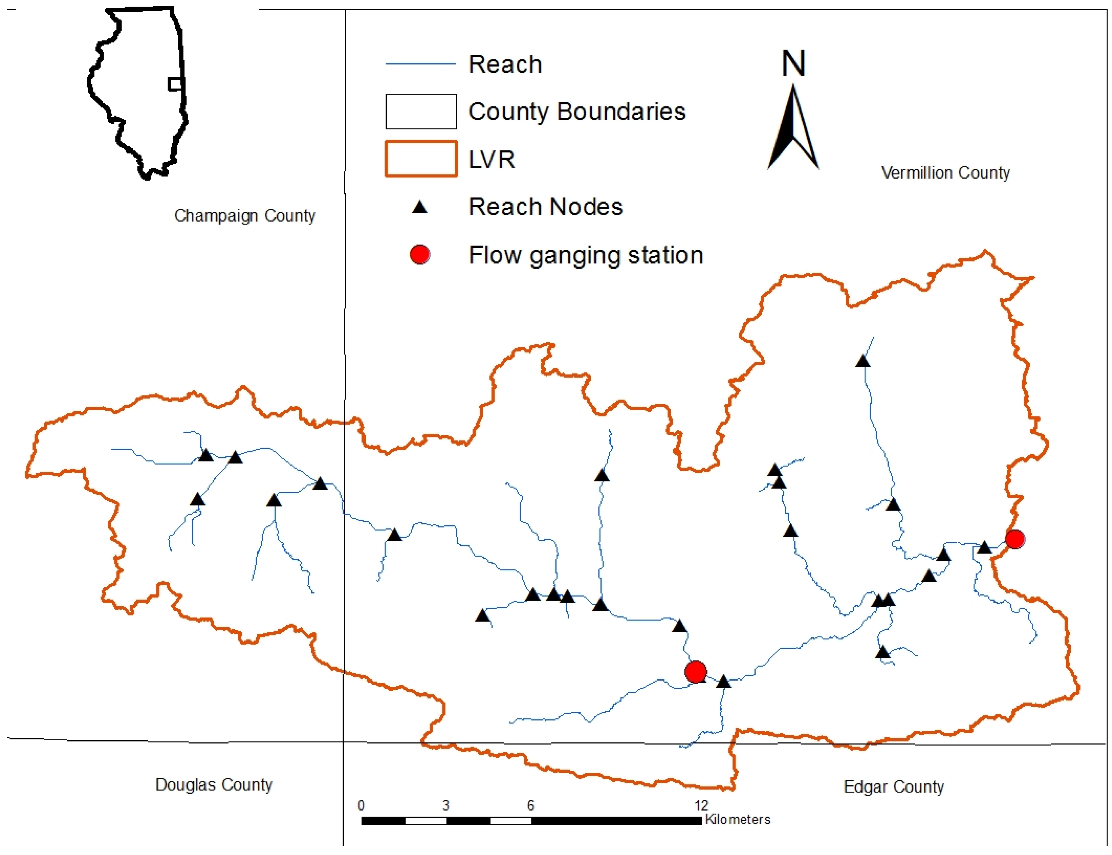
The Little Vermillion River (LVR) watershed covers an approximately 489 km
2 area and is located primarily within Vermillion County, IL, though it stretches into nearby Champaign and Edgar counties (
Figure 1). It is an agriculturally-dominated watershed with the primary crop rotation of corn and soybeans, with the average annual rainfall of 1040 mm. The majority of the watershed has slopes of less than 1%, with the dominant soil series being Drummer silty clay loam and Flanagan silt loam series. With the majority of the watershed being flat and covered with poorly drained soil, man-made tile drainage was required to convert them to high quality agricultural land. This has led the majority of the hydrology to be altered so that most of the water is drained by tiles into man-made ditches. Watersheds like LVR contribute to the hypoxic zone formation at the Gulf of Mexico. Another problem associated with this watershed has been found with a reservoir located near Georgetown, Illinois. The water from this reservoir is used for drinking purpose and has tested positive for elevated levels above the maximum contaminent level (10 mg/L) for nitrate.
The LVR water quality monitoring project was started in 1991 by the University of Illinois as a long-term water quality and flow monitoring project [
7]. Seven subsurface and four surface monitoring stations were established at farms located within the watershed, with two river stations located at various distances from the river source. These farms also provide management operation information. The outlet river station for this model is located upstream of a dam before LVR crosses into Indiana. This station was established in 1996 and continued through the end of 2000, but there were problems at the beginning of station operation and that were not fixed until mid-1997. Flow and nitrate data from an additional monitoring station located within the watershed was used as a supplemental to the outlet data for calibration and validation for 1998–2000 duration.
2.2. Hydrologic Model Equations
Currently, SWAT 2012 gives users the option for tile drainage to be modeled using DRAINMOD modeling routines [
8]. This modified SWAT tile drainage option uses Hooghoudt’s steady-state equation to compute both drainage and sub irrigation flux and Kirkham tile drainage equation. These equations use the effective horizontal hydraulic conductivity in order to evaluate the flux between the water table level at the midway point between drains and the hydraulic head in the tiles. The Hooghoudt equation is represented as follows:
where
q is the drainage flux (mm/h), m is the water table height above tile depth at the midpoint between tiles (mm),
Ke is the effective lateral saturated hydraulic conductivity (mm/h),
Ltile is the distance between the tiles (mm),
C is the ratio of the average flux between the tiles to the flux midway between the drains, and
de is the equivalent depth in order to correct for convergence near the tiles (mm). The equivalent depth (
de) is obtained using the equations developed from Hooghoudt’s solutions by Moody (1966) as a function of
L,
d, and tube radius (
r) [
8].
When the water table reaches the surface and ponded water remains for relatively long periods of time, modified SWAT switches to using the Kirkham equation:
where
t is the depth of the ponded water (mm),
b is the depth from the surface to the midpoint of the tile (mm),
r is the radius of the tile (mm), and
g is a dimensionless factor determined using an equation developed by Kirkham [
8].
2.3. Nitrate Model Equations
The discharge of NO
3 into tiles is based on the concentration of NO
3 in the soil water near the tiles. The initial nitrate levels, which are the primary form of nitrogen that plants uptake, have an inverse exponential relationship with depth [
9]:
where
NO3conc, z is the initial concentration (mg/kg or ppm) of nitrates at a depth
z (mm).
Only part of NO
3 is actually mobile and thus available for discharge through the tiles. The concentration of nitrates in mobile water is calculated by the equation:
where
is the concentration of nitrates in mobile water for a given layer (kg N/mm H
2O),
is the amount of nitrates in the layer (kg N/ha),
is the fraction of porosity in which anions are excluded, and wmobile is the amount of mobile water in a layer (mm) [
9]. The concentration of NO
3 in the flow entering the tile is assumed to be the same as the concentration of mobile water.
2.4. SWAT Model Setup
2.4.1. Input Data
This study uses ArcSWAT 2012 (revision 637, College Station, TX, USA) extension for ArcGIS 10.1 (ESRI, Redlands, CA, USA). Most of the input data needed for SWAT can be obtained from publically available internet sources. A 10 × 10 meter resolution Digital Elevation Model (DEM) and National Land Cover Data (NLCD) 2006 were obtained from the USGS seamless survey [
10]. The SWAT model uses the DEM data to determine the direction and accumulation of water flow [
10]. Data sets were re-projected into the NAD 1983 UTM Zone 15N projection for more accurate measurements.
In order to create hydrologic response unit (HRU) in SWAT model, additional data about land cover and the soils were needed. The NLCD data provides some basic information about land usage, but agriculture is defined generically. Therefore, cropland Data Layers (CDL) from the USDA National Agricultural Statistics Survey was combined with 2006 NLCD data [
11] as outlined by Winchell
et al. [
12]. Cropland data for 1999–2003 duration was used to create a 4 year crop rotation for the agricultural land. Before combining the CDL layers to determine crop rotations, values were reclassified to assume anything that was not corn or soybeans to be insignificant (Raster value zero). To combine the data layers, the raster calculator used the equation CDL 1999 × 1000 + CDL 2000 × 100 + CDL 2001 × 10 + CDL 2002 × 1 in order to determine the rotation. If at least three years were not planted as corn or soybeans, it was assumed that CDL 1999 data held throughout the period. The determined crop rotation replaced the agricultural area in the NLCD data set. A custom look table needed to be created for this new data set, combining the NLCD lookup table with the CDL rotation table. Soil data for the Illinois counties of Champaign, Edgar, and Vermillion was obtained from the Soil Survey Geographic Database (SSURGO).
Daily temperature and precipitation was obtained from USDA Agricultural Research Service (ARS) on a county wide basis [
13]. Data sets for Champaign, Vermillion, and Edgar counties were obtained and combined into temperature and precipitation lookup tables. The other weather data sets (weather generator, relative humidity, solar radiation, and wind speed) can either be derived from observed data sets or simulated. This study used the WGEN_US_COOP_ 1960_2010 monthly weather database to obtain simulated values for relative humidity, solar radiation and wind speed.
2.4.2. ArcSWAT Interface Setup
Before SWAT delineates streams and outlets, SWAT requires an area of flow accumulation in hectares (ha) to delineate the main channel, tributaries based on defined outlet. For this study, flow accumulation area was assigned to be 388 ha generating 37 subbasins. Before HRUs could be classified, the DEM had to be separated into different slope classes. The mean slope for the watershed was found to be 1.1%, with the maximum slope being 100%. This study used three slope classes, with the upper limits of the slope classes being 1%, 5% and 100%. In order to create hydrologic response unit (HRU) with unique soil, landuse and slope combination, 15% threshold for landuse, 10% for the soil and 35% of the slope threshold was used, with an exception to urban land and water. A total of 417 HRUs was created using this definition.
After the weather data definition was complete, agricultural management practices were entered into the model. Since the agricultural area in the watershed is artificially drained via tiles, subsurface drainage tiles were implemented at 1 m depth and 30 m apart with time to drain to field capacity at 24 hours and a drainage lag time at 48 hours for agricultural area. Based on the area, the effective drainage radius was set at 25 mm, and the multiplication factor for determining the saturated lateral hydraulic conductivity from the SWAT input for saturated hydraulic conductivity (LATFSATK) was set at 2. The crop rotation management operations for the agricultural lands were derived from stations in the watershed for the period from 1995 to 2000. The tillage operations were assumed to be conventional tillage for the agricultural area based on field station management data. The conventional tillage operations included ammonia application before corn planting, pre-planting field cultivator tillage operation, a row cultivator tillage operation 2 months after corn planting, and a post-soybean harvest fertilizer application of a low nitrogen-phosphorus mixture, which is followed by a v-ripper tillage operation.
2.4.3. SWAT Calibration and Validation
Because of the large number of model parameters, an automatic calibration program (SWAT-CUP) was used for calibration and validation. A rank sensitivity test was performed for all parameters for flow and nitrate (NO3) to determine the sensitivity of the different parameters. The model was calibrated for 1998 and validated for 1999–2000 using flow and nitrate data at the outlet. Similalrly, a SWAT CUP calibration run also included flow and nitrate data from another station located at the midpoint of the watershed, covering about 49% of the total area of the watershed for 1996–1998. The parameters for the best simulation determined by SWAT CUP were tested for 1999–2000 data validation for this station.
Nash-Sutcliffe coefficient was used as the calibration reference to determine the best parameters. Nash-Sutcliffe (NS) coefficient is commonly used goodness of fit measure for hydrologic and water quality models. The closer the NS value is to 1, the more the simulated values correlate with the observed data. The NS value can be computed with the equation:
where
Ef is the efficiency index or NS,
and
are the predicted and measured values of the dependent variable
is the mean of the measured values, and
n is the sample size [
14].
Another statistic used to determine calibration is percent bias. Percent bias (PBIAS) measures the percent deviation of the simulated data compared to the observed data [
14]. The PBIAS value can be either positive or negative, with a positive value indicating an underestimation and a negative value indicating an overestimation of the model. On a monthly basis, the absolute value of PBIAS should be less than 25% for flow and 70% for nutrients. The equation for calculating PBIAS is as follows:
The parameters looked at were determined to be the most sensitive based on a review of previous studies done by Arnold
et al. [
15]. The automatic calibration program SWAT-CUP’s SUFI calibration procedure modifies the model parameters for each iteration, and then it determines the best parameters based on NS value. Ten SWAT-CUP simulations were run for each parameter modified.Based on these iterations, SWAT-CUP performs both a T-test and a p-test. If a parameters
p-value is less than 0.05, that parameter was considered to be not significant. Parameters considered to be significant based on SWAT-CUP
p-values, their range and calibrated values are listed in
Table 1.
2.4.4. Best Management Practices Implementation
Tillage is a common land management operation used to loosen the soil for planting as well as to mix the fertilizer into the soil. By reducing tillage, the soil is less disturbed and will be less able to erode the soil and the nutrients within. In order to understand the effect of tillage management on nitrate load, reduced and no tillage scenarios were investigated based on commonly used land management in the region. Reduced tillage operations entailed a pre-corn ammonia fertilizer application, pre-planting field cultivator tillage operation, post-soybean harvest low nitrogen phosphorus mixture, and a post-harvest v-ripper tillage operation. No tillage operations had a side dressing of ammonia applied to corn 1–2 months after planting and a post-soybean harvest fertilizer application of a low nitrogen phosphorus mixture.
Filter strips are another commonly used practice in order to reduce pollution. The filter strip is presented in SWAT model as an area ratio of the HRU to filter strip (X:1) [
16]. Common ratios range from 30–60, with 40 being the default value. Ratios tested are 20, 40, 60, and 80. Filter strips are placed in the .ops input files.
Wetlands were implemented using the information on surface area and volume obtained by a field study by Miller [
17] located near LVR. The field study area done by Miller [
17] drained a 10.9 ha field, with the wetland having a normal surface area of 177 m
2 and a volume of 56 m
3. The SWAT Input/Output documentation suggests the settling rate for nitrogen and phosphorus in the Midwest is 12.7 m/year [
16]. Different wetland scenarios tested were 0.16% of subbasin normal surface area 32 cm volume, 0.16% of subbasin normal surface area 16 cm volume, 0.32% of subbasin normal surface area 32 cm volume, and 0.16% of subbasin normal surface area 64 cm volume. Wetlands were included in the .pnd input files.
Another BMP tested was the use of cover crops after the harvesting of the main crops. Cover crops add extra organic matter to the soil because they are not harvested but killed and incorporated prior to main crop planting. Two different cover crop scenarios were tested. The first scenario uses just rye as a cover crop, while the second scenario uses rye after corn and red clover after soybeans. Rye would utilize unused nitrogen from after corn from the fertilizer. For red clover, the amount of nitrogen fertilizer would need to be less due to nitrogen fixation by red clover.
To determine statistical significance of each BMP, statistical tests were conducted on annual basis. Using the actual weather information, the calibrated/validated model was run for 1980–2009 to simulate flow and and nitrate load for various BMP scenarios, allowing for a wide variety of precipitation years to be simulated. The statistical test was done using a paired Wilcoxon test. The Wilcoxon [
18] statistical test is a common way for determining the statistical significance of paired data whether they came from the same source or not. The simulated BMP result was compared to the calibrated (conventional tillage with no additional BMP) model in order to determine if the changes in flow and nitrate load were statistically significant. If the
p-value is above 0.05, the BMP was not considered to be statistically significant compared to the calibrated model scenario. Additionally, the two best scenarios were combined in order to determine the effectiveness of the combined BMPs.
3. Results
3.1. Calibration and Validation
3.1.1. Outlet Flow
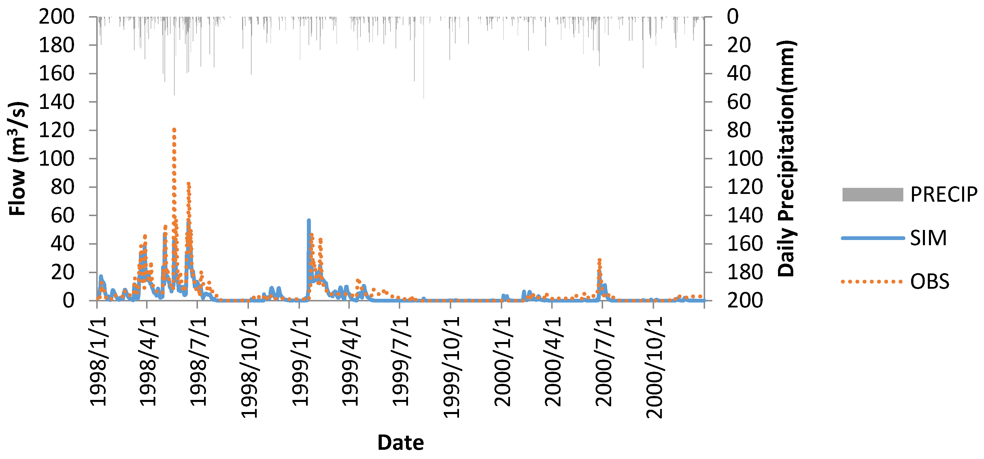
The SWAT model has a tendency to underestimate the peak flow in the wet year (1998) when compared to the observed data, while non-spring peak flows tend to be overestimated with nonevents sometimes being simulated in the non-growing season (
Figure 2). The mass balance comparison reveals most of the mass difference does not occur from the peak storm events, but from periods following peak storm events.
The calibrated SWAT model has a daily NS value for the outlet station of 0.67 for the calibrated period of 1998 and 0.44 for the validation period of 1999–2000. The reason that the validation NS is small is because compared to the other two years, 1998 was a wet year with multiple peak events recorded. With much less fluctuation, the small differences have a greater impact on the NS number than in wet years. The calibration parameter values for the outlet on a monthly basis are 0.76 for the calibration period and 0.67 for the validation period. For the upstream station, computed NS value was 0.55 for the calibration period of 1996–1998 and 0.63 for the validation period of 1999–2000. Based on Moriasi
et al. [
14], the model performance rating on a monthly time step based on NS would be considered good for both the calibration and validation periods. Based on PBIAS, the model’s results would be satisfactory for the calibration period and good for the validation period.
3.1.2. Outlet Nitrate Discharge
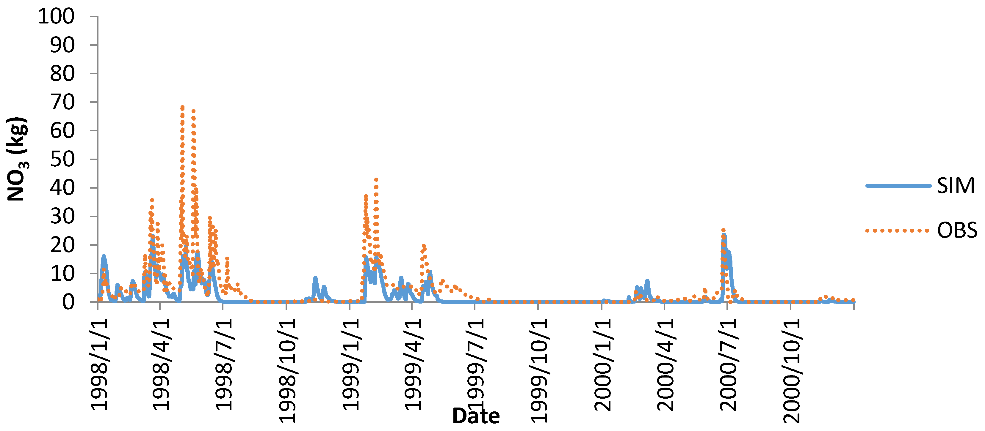
Unlike flow, SWAT tends to underestimate the peaks of nitrate discharged (
Figure 3).
The new tile drainage routines were used in an attempt to more realistically model nitrate discharge in tile flow. Because fertilizer application timing and rate is not uniform across the watershed, this might have lead to discrepancy between observed and simulated nitrate discharge. The calibrated model has an outlet daily NS of 0.35 for the calibration period and 0.44 for the validation period The midpoint station has a NS of 0.36 for the calibration period and 0.26 for the validation period. On a monthly basis, the NS values are 0.52 and 0.51 for calibration and validation periods, respectively. Based performance ratings given by Moriasi
et al. [
14], the monthly model would be satisfactory for both the calibration and validation periods.
3.2. Best Managemen Practices Analysis
Table 2 shows the Wilcoxon test for all the BMPs on a yearly basis. All BMPs simulations were found to be statistically significant on a yearly basis for nitrate discharge compared to the default of no BMP and conventional tillage, while all BMPs except filter strips and reduced tillage were also statistically significant for flow.
3.2.1. Tillage
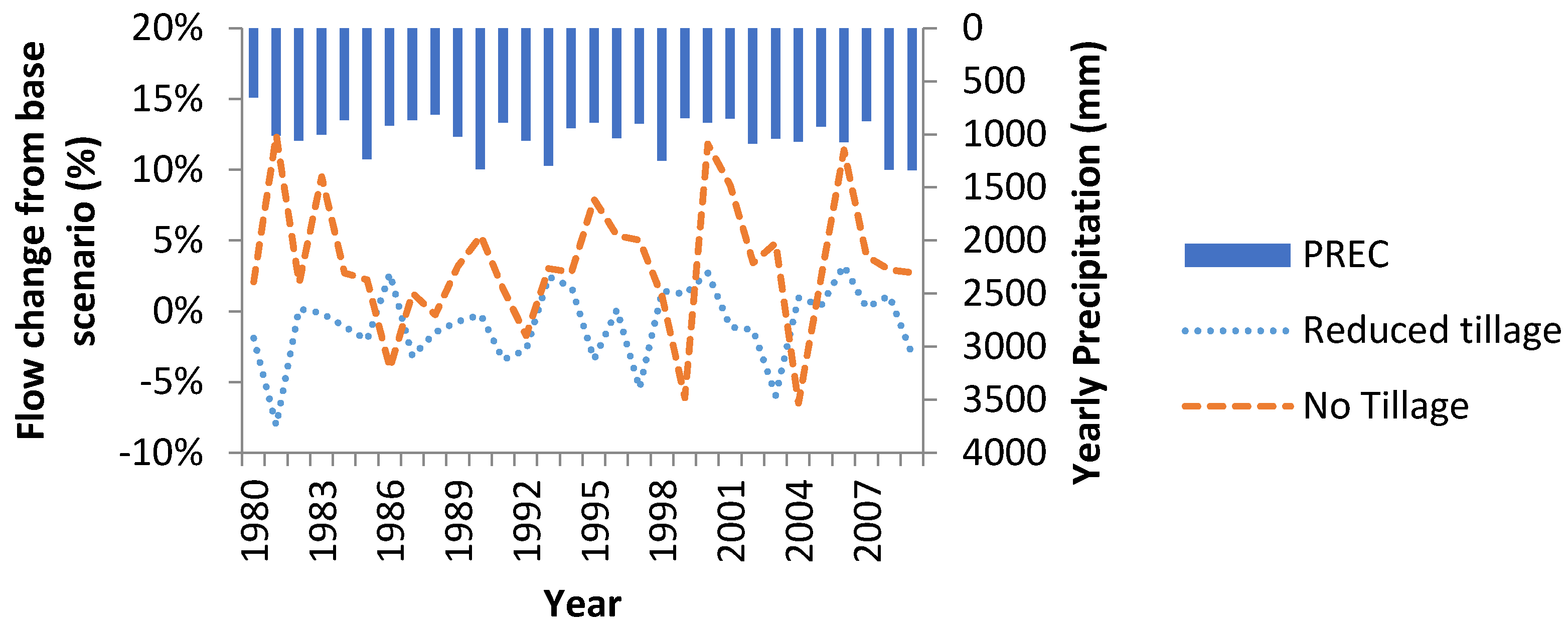
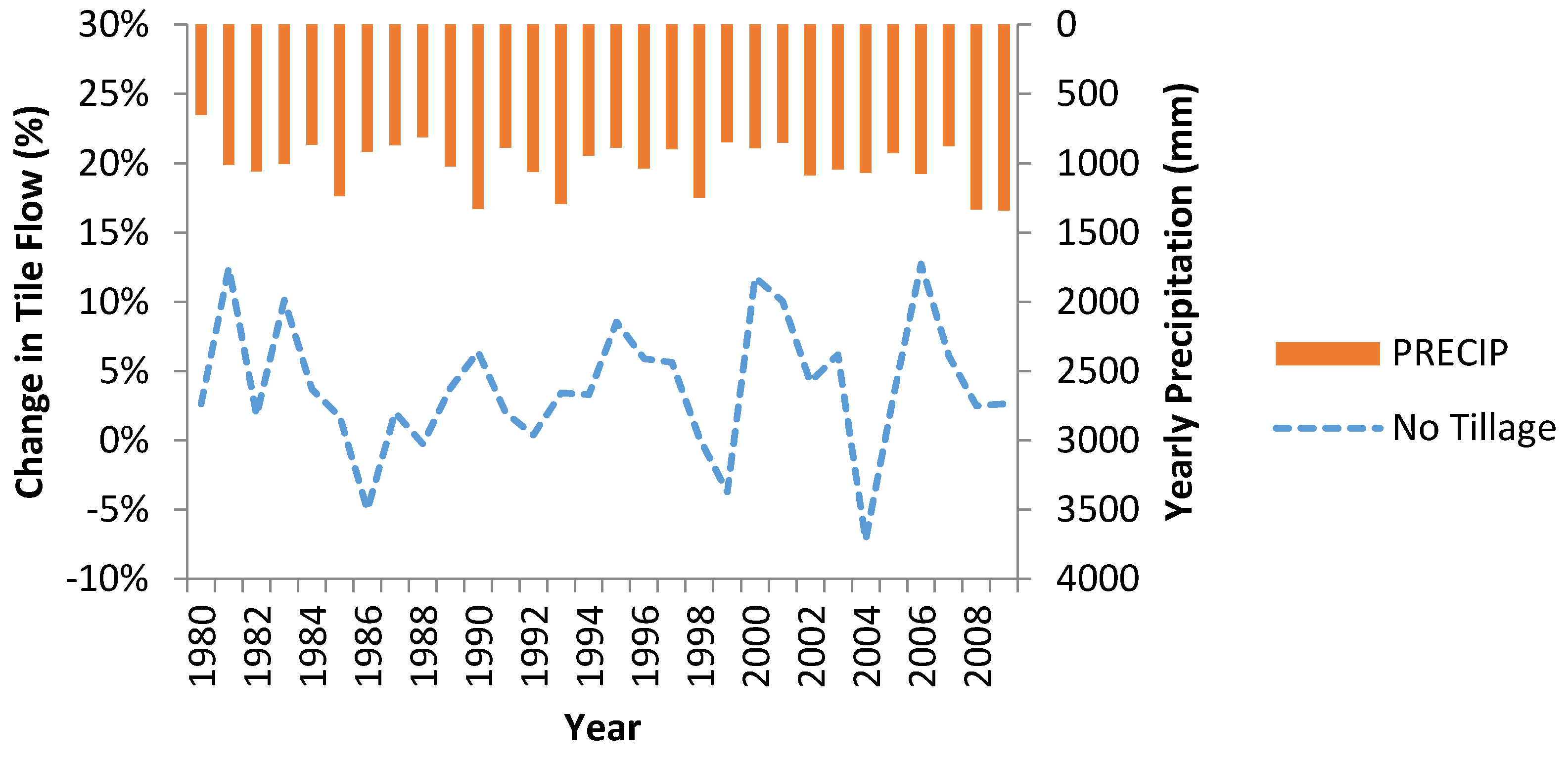
Figure 4 shows the impact of changing from conventional tillage to reduced tillage and no tillage operations on watershed outlet flow without implementing any additional BMPs. No tillage shows an increase in flow, while reduced tillage shows little change to flow (average annual increase in flow −0.54%
vs. 2.8%). It was also observed that the increase in flow was correlated with increased tile drainage for no tillage practice (an average increase of 3.3%) (see
Figure 5).
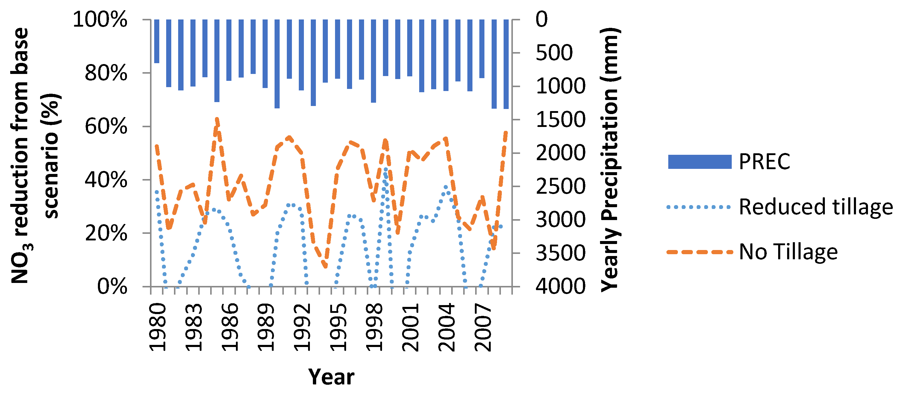
Figure 6 shows the change in nitrate discharge at the watershed outlet due to change in tillage practice (average annual decrease 15% for reduced tillage
vs. 43% for no tillage). With the improve soil structure as well as more optimal timing of fertilizer usage, no tillage shows a significant decrease in the amount of nitrogen discharged at the watershed outlet.
3.2.2. Filter Strips
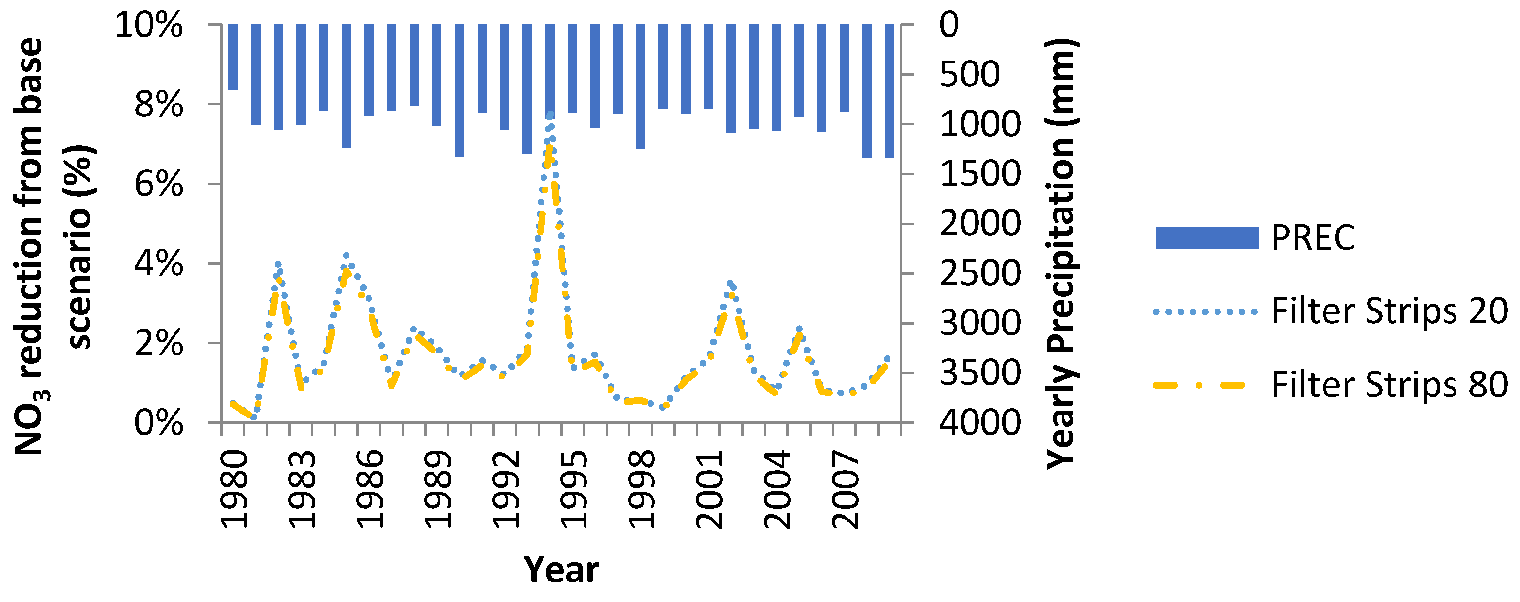
Though filter strips are a commonly used BMP, their usefulness in nutrient reduction in a tile-drained watershed is minimal. Since most of the nutrients are discharged via tile drainage instead of surface runoff, only a small amount of nutrients can be removed (average annual nitrate decrease for filter strip sizes are 1.7%, 1.6%, and 1.5% for the ratios 20, 40, and 80, with 60 having similar results to 40). Filter strip size does not significantly matter since only nitrate discharge in surface flow can be removed, and much of that is already removed with smaller filter strips (
Figure 7).
3.2.3. Wetlands
Since only surface runoff is assumed by SWAT to enter the wetlands, nitrate reduction potential is limited (average annual nitrate reduction is 1.1% for 0.16% 32 cm, 0.9% for 0.16% 64 cm, 1.4% for 0.16% 16 cm, and 1.3% for 0.32% 32 cm). A lower ratio of wetland normal surface area to volume is desirable for nitrate reduction, with weltand area being slightly less sensitive (
Figure 8).
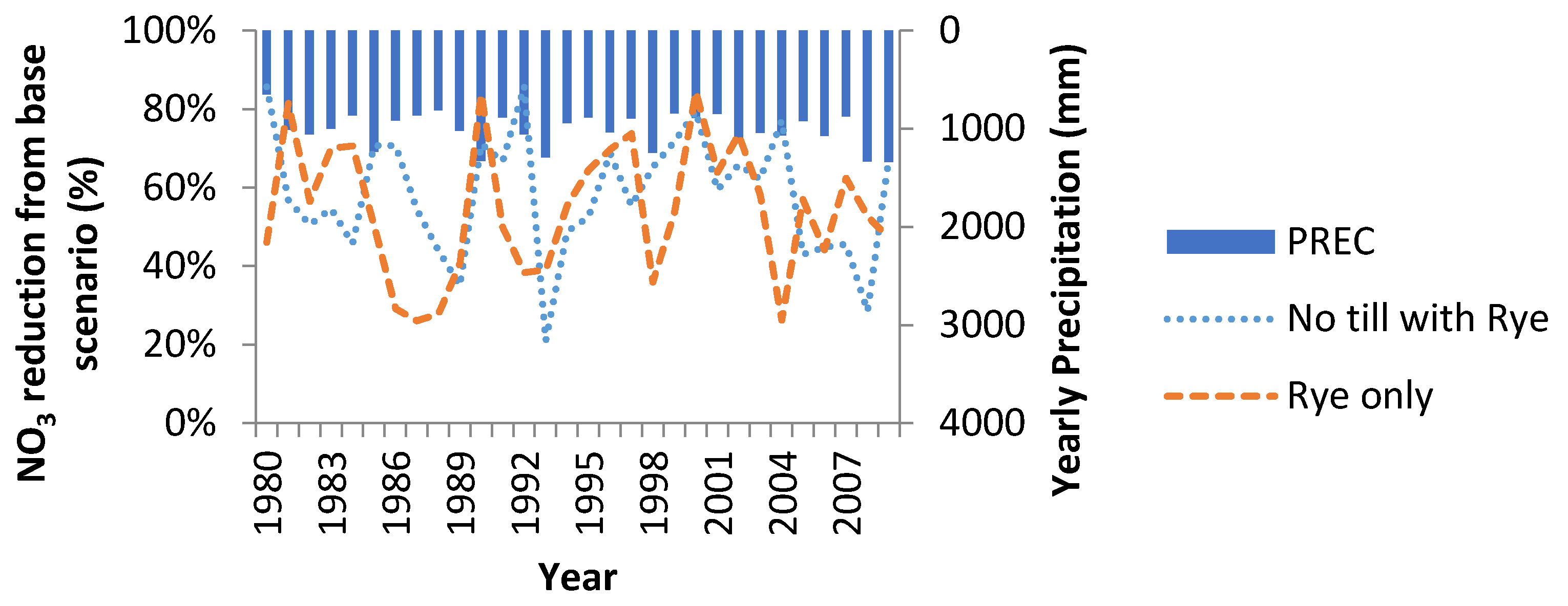
3.2.4. Cover Crops
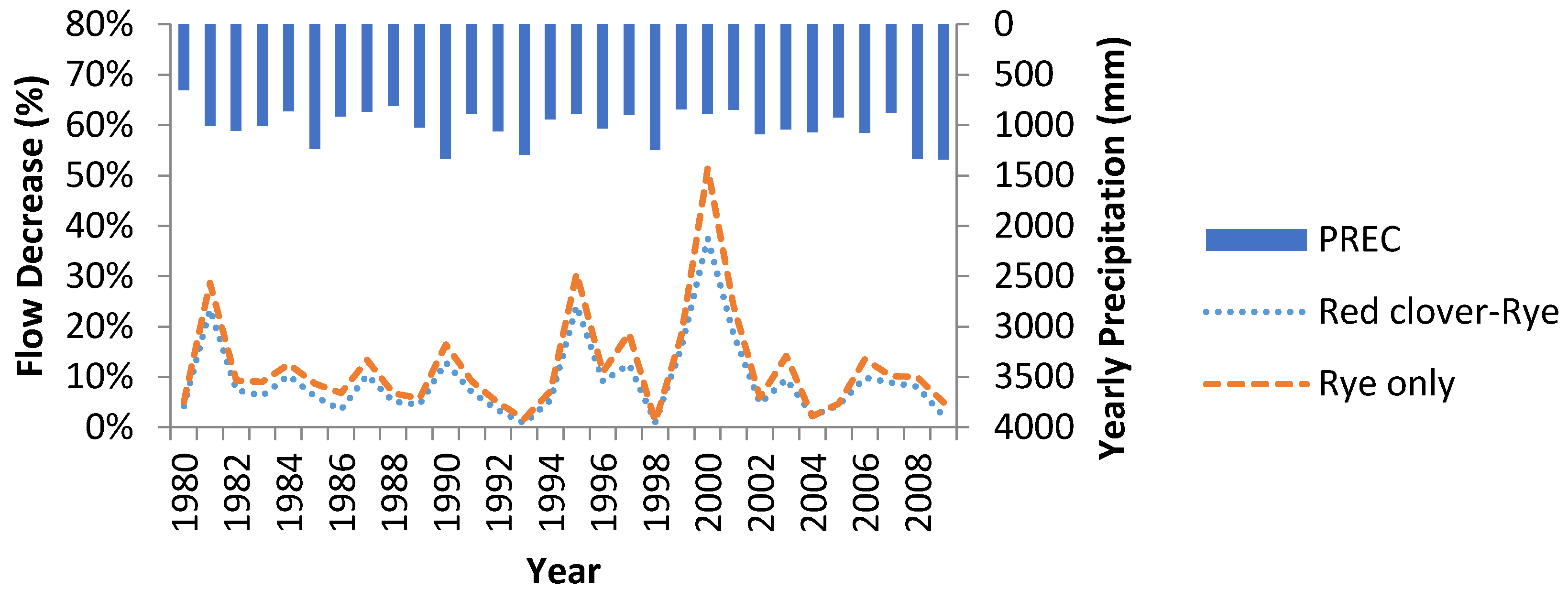
On a yearly basis, using only rye as a cover crop does better than using a rye-red clover cover crop rotation and reducing fertilizer nitrogen input by 56 kg/ha (about 50 lbs) (average annual reduction for rye only is 54.5%
vs. 24.5% in the red clover-rye cover crop rotation). The use of cover crop reduces the amount water discharge to the stream due to continuous uptake of water for transpiration and photosynthesis throughout the year (see
Figure 9) (an average annual flow reduction of 7.2% for the use of red clover and rye and 9.5% for rye alone). The use of a nitrogen scavenger like rye reduces nitrate discharge because the fertilizer left over after corn harvest will be utilized by the rye before it is reincorporated into the soil as organic nitrogen (see
Figure 10).
3.2.5. Multiple BMPs
The addition of no tillage to Rye cover crops has a variable impact on nitrogen reduction, with no disnerable wet or dry pattern detectable (
Figure 11). Over the 30-year average, the combined BMPs do perform better at reducing nitrates than Rye cover crops by itself (an average annual improvement of 13% compared with rye only).
4. Discussion
4.1. Calibration and Validation
4.1.1. Outlet Flow
The SWAT model had a tendency to mostly underestimate peak flows, though a sometimes overestimates them. The model also does not accurately model the baseflow, with flow dropping quicker than data shows. The review of SWAT’s new tile drainage equations by Moriasi
et al. [
8] found overestimation of monthly peaks. Zhao
et al. [
19] also found overestimation for the peaks, but simulated results followed the observed data through the rest of the simulated period. Sahu and Gu [
20] likewise found an overestimation of flow, especially for the wet years. This could be caused by an incorrect determination of when the conditions are wet, dry, or normal for adjusting the curve number. A calibration was tested for determine the curve number adjustment based on evapotranspiration rather than soil moisture, but the best parameters for evapotranspiration based curve number adjustment did not produce a better model than soil moisture based curve number adjustment. Another possibility could lie with the curve number method itself. Accuracy is sacrificed for the sake of simplicity in the curve number method.
One option to consider would be using the Green-Ampt infiltration equation, which is included as an option in SWAT. Green-Ampt requires precipitation data to be in a sub-daily time step. King
et al. [
21] compared the two methods in a watershed in north central Mississippi. On a monthly basis, the curve number method performed better than Green-Ampt and was a tighter fit despite underestimations. Ficklin and Zhang [
22] compared the two methods in SWAT uncalibrated on the San Joaquin River watershed in California and found that Green-Ampt was slightly less effective overall but performed better for large storm effects but its effectiveness decreases with increasing watershed size and is not appropriate for simulating watersheds with a lot of saturated areas. Due to lack of hourly weather data that is required for Green-Ampt, it could not be incorporated into this model.
The SWAT model has a tendency to overestimate peaks during the non-growing season and models a quick drop-off in flow. It was suggested by Moriasi
et al. [
8] that increasing the spacing between drains could help mitigate these errors. The most sensitive tile drainage parameter that they found was drain spacing, with the optimum drain spacing in their study which used an Iowa watershed being 25 m. For this study, the most sensitive parameter was found to be LATK, though tile drainage spacing’s sensitivity was the second most sensitive tile drainage parameter.
4.1.2. Outlet Nitrate Discharge
Inaccuracies in peak modeling lead to difference in the mass balance between the observed data and simulated results. This could be due to the inaccurate modeling of pollutants in tile drainage discharge or tile drainage itself. Another possible explanation is the actual non-uniformity of fertilizer application rate and timing could have a greater impact than can be represented in the model. For total nitrogen discharged, Zhao
et al. [
19] actually found a tendency of SWAT to overestimate. This could suggest a tendency of SWAT’s nitrogen cycle modeling routine to underestimate the transformation of nitrogen from nitrates to other forms. The model performance in this study could suggest the opposite in the potential transformation of nitrogen, with inaccuracies due to overestimations in modeling of denitrification, underestimations of mineralization, and/or overestimation of the crop’s efficiency in utilizing fertilizer nitrogen.
Using the old tile drainage routines on a comparative study of two tile-drained watersheds in Quebec, Gollamudi
et al. [
23] reported that SWAT continually underestimating the nitrate load peaks throughout the simulated period on both watersheds. These underestimations were hypothesized to be a result of SWAT’s inability to match water yield for those months or small errors in fertilizer load estimation. However, Sahu and Gu [
20] observed the opposite result for their Iowa study. Their un-calibrated model for nitrate discharge found SWAT overestimating the cumulative nitrates at the outlet, with the model having a relatively good NS for nitrates of 0.87. They mentioned that, since fertilizer application timing is not spatially uniform, the way the modeler handles that will affect nitrate discharge. Recorded field operations for conventional tillage vary with application timing, with the 1998 and 1999 application of nitrogen on corn being applied after corn planting rather than preplanting or fall application like with other years. However, the flow station located within the watershed shows that the underestimation is not exclusive to 1998 and 1999, as it also occurs for 1996 and 1997, leading to the hypthothesis that side dressing instead of traditional application could not be responsible for the majority of the differences in observed
vs. simulated nitrate discharge.
The new tile drainage routines were used in an attempt to more realistically model nitrate discharge in tile flow. Because fertilizer application timing and rate is not actually uniform across the watershed, some amount of user error was introduced in trying to calibrate the model for nitrate discharge.
4.2. Best Managemen Practices Discussion
4.2.1. Tillage
Since reducing tillage operations was simulated to increase tile drainage flow, the drainage of the soil must be improving. Tillage removes larger pores when disturbing the soil in order to make planting easy or mix in fertilizer into the soil. Reducing tillage will reduce these disruptions but not eliminate them. This improved drainage allows for tiles to be more efficient during dry years and drain the field to field capacity more effectively. The conservation of macropores reduced the overall field capacity of the soil compared to conventional tillage removing them.
Tan
et al. [
24] reported that no tillage results in greater preferential flow as a result of increased earthworm population as well as possible improved pore continuity in the long term. The SWAT simulation of Lake Erie basins by Bosch
et al. [
25] found little impact to total flow by no tillage practices. However, field data from Francesconi
et al. [
26] showed little difference in annual tile fow between reduced and no-till field plots. Our simualated results agree with Tan
et al. [
24] results, though further study into the effects of tillage in modeling tillage drainage may need to be done.
Despite the increase in tile flow, the discharge of nitrogen actually decreased due to more efficient usage by the crops. More nitrogen is held close to the surface where it can be more effectively utilized by crops early in the growing cycle rather than distributing them in the soil profile. Improved aeration by increased earthworm activity helps the root to access more macro pores, which are reconfigured by tillage practices. These observations suggest that no tillage can improves crop nitrogen utilization. Tan
et al. [
24] found opposite results in their field study, where the no till plots had more nitrate discharged than the conventional tillage plots in tile flow. Chung
et al. [
27] found similar results to SWAT’s simulated data in that nitrate discharge by no tillage management practices was reduced in a soybean-corn rotation when compared with conventional tillage. A study by Bosch
et al. [
25] showed little impact of a no-till system on nitrate discharge between calibrated and simulated model. Looking at two Indiana watersheds, Kalic
et al. [
28] actually saw a small average annual increase in nitrate export compared with conventional tillage, though their conventional tillage practices involved only tillage operations involved with incorporating the fertilizer into the soil. Compared with reduced tillage, Francesconi
et al. [
26] found in field studies a significant reduction in nitrates discharge in no tillage practices compared to reduced tillage. Part of the yearly variation from the default of conventional tillage is due to the assumed fertilizer application rate being more variable from year to year than the other tillage practices. No tillage also had a lower yearly average application rate than reduced no tillage. With the phosphorus fertilizer application taking place in spring pre-plant of corn and nitrogen fertilizer always being applied as side dressing during the early growing season, corn has more oppurtunities to utilize the fertilizer before it can leach through tile drainage than in conventional tillage. Taking the percentage of fertilizer discharge from the outlet over the 30 year average, conventional had an amount of nitrates discharged equivalent to 27% of applied nitrogen fertilizer , while reduced and no tillage had 23.5% and 18.9% equivalent of nitrogen fertilizer discharged, respectively.
4.2.2. Filter Strips
Since runoffa significant amount of nitrates is simulated to be discharged through tile drainage rather than surface runoff, only a small amount of nitrates can be removed through filter strips. Filter strip size does not significantly matter since only nitrate discharge in surface flow can be removed, and much of that is already removed with smaller filter strips (see
Figure 7). In the Bosch
et al. [
25] study, the filter strip with a 25% trapping efficiency managed to remove about 14% of nitrogen discharged from surface flow. Sahu and Gu [
20] found some subbasins in their model of the Walnut Creek watershed in Iowa had upwards of 80% of nitrate removed in a normal year for filter strips with a ratio of 10 on a moderately well drained soil. Both of these studies used an older version of SWAT’s filter strips routines and mainly dealt with non-tile drained areas when evaluating the filter strips. Kalic
et al. [
28] reported small decreases in nitrate discharge in both watersheds simulated slightly less than simulated average annual decreases in LVR.
4.2.3. Wetlands
Miller [
17] demonstrates reductions of about 35% due to tile drainage rather than surface runoff being collected and stored in the wetland. While investigating the effects that wetland restoration on water quality in the Little Saskatchewan River, Wang
et al. [
29] reported a reduction in both nitrogen and phosphorus up to 25% on an average annual basis with an increase of total area draining into wetlands of 3103 ha. Their first study watershed experiences a 120 m drop in elevation, with greater snowfall and a much colder climate than LVR. It also contains less agriculture than LVR and a different soil type. These factors are the reason why discharge from their study watershed is much lower than from LVR. Wang
et al. [
29] concurrently developed a comparison model to simulate the effects of removing wetlands in a similar watershed based in Minnesota; the simulated results showed an increase of nitrogen and phosphorus loading of 22% and 25%, respectively, which concur with the decrease from their other watershed. The larger pollutant load of LVR compared with these watersheds and the assumption that only the surface flow of LVR would flow through the wetland BMP could explain the differences between the studies. An Indiana study by Kalic
et al. [
28] found slightly better nitrate reduction from wetlands, though concurs with the analysis that SWAT needs to allow for tile drainage to enter wetlands in order to obtain a better simulation.
4.2.4. Cover Crops
Rye as a cover crop preformed better than used in a cover crop rotation with red clover and an associated decrease in nitrogen fertilizer usage. Even the cover crop of rye after corn would not be able to scavange all of the nitrogen fertilizer that was not leached through tile drainage during the growning season or utilized by corn. An additional year’s worth of rye allows for more scavenging of any nitrogen fertilizer still in the soil matrix after soybeans (which do not use the fertilizer). Since the rye is killed and not harvested, all of the nitrogen scavange is recycled to organic nitrogen pool. Dryer years causes valleys in nitrogen reduction from rye because rye’s effectiveness at scavenging nitrates is reduced by dryier conditions. A SWAT study by Kalic
et al. [
28] also found that the use of rye as a cover crop helped in reducing nitrate load, though their simulated percentage reduction was found to be less than half of LVR’s simulated reduction.
4.2.5. Multiple BMPs
Because one of the purposes of cover crops is to increase soil organic matter, combining no tillage management practices with rye as a cover crop does little to improve nitrate reduction. The management practices of no tillage already allow for better effective usage of nitrogen fertilizer by corn, leaving less nitrogen avaible to be scavenged by rye. After the kill operation, the rye residue is left on top of the soil rather than being incorporated into the soil with a tillage operation. The lack of incorporation into the soil makes the process in which the nitrogen scavenged by the rye available to the main crop’s usage to be a slow process. When the nitrogen becomes plant available again, it allows for rye to become more effective in scavenging leftover nitrogen fertilizer.
5. Conclusions
We investigated the impact of BMP implementation on water quality from a tile-drained watershed using SWAT model. Among the BMPs simulated, rye as a cover crop was found to be the best BMP to reduce nitrate load among the BMPs tested. By utilizing nitrogen from fertilizer that was not used by corn but still within the soil matrix, rye is able to remove the mobile nitrates and increase the amount of soil organic matter, improving the soil’s structure. No tillage practices also decrease the amount of nitrates discharge significantly. By not disturbing the soil, macro pores are kept intact, allowing for preferential flow paths, improved root aeration, increased earthworm activity, and improved soil structure to occur. With plant roots able to get better established as well as improved fertilizer scheduling, nitrates are able to be more effectively utilized by corn compared to the conventional tillage system. Though filter strips perform well in other watersheds, their effectiveness is minimal in a primarily tile-drained watershed. Wetlands reduce pollutants discharged from the watershed, but SWAT would require a modification so that tile flow could be stored in wetlands before entering the reach. A combination of rye as a cover crop and no tillage yielded mixed results with regards to nitrates discharge. Better utilization of nitrogen fertilizer by the corn because of the increased accessibility of nitrates combined with the lack of incorporation of rye as organic matter with tillage makes the combination of the two BMPs vary with effectiveness compared to utilizing rye as a cover crop alone.
By understanding the results of this study, County Extension offices in the immediate area of the study watershed would be able to use the results of this model to recommend to farmers methods of reducing nitrogen pollution discharged from their farms. Future studies in the near by region should be able to use the calibrated and validated parameters from this study as a reference point, while concurrently providing management guideline to reduce nutrient load.
Acknowledgments
We acknowledge the support provided by the USDA National Institute of Food and Agriculture, Hatch project ILLU-741-379 to cover the publication cost.
Author Contributions
J.M. conducted the study and wrote the paper under the supervision of P.K and R.B.
Conflicts of Interest
The authors declare no conflict of interest.
Abbreviations
The following abbreviations are used in this manuscript:
| LVR | Little Vermillion Watershed |
| SWAT | Soil and Water Assessment Tool |
| BMPs | Best Management practices |
| GIS | Geographical Information System |
References
- Rabotyagov, S.; Campbell, T.; Jha, M.; Gassman, P.W.; Arnold, J.; Kurkalova, L.; Secchi, S.; Feng, H.; Kling, C.L. Least-cost control of agricultural nutrient contributions to the Gulf of Mexico hypoxic zone. Ecol. Appl. 2010, 20, 1542–1555. [Google Scholar] [CrossRef] [PubMed]
- Aulenbach, B.T.; Buxton, H.T.; Battaglin, W.A.; Coupe, R.H. Streamflow and Nutrient Fluxes of the Mississippi-Atchafalaya River Basin and Subbasins for the Period of Record through 2005; U.S. Geological Survey Open-File Report 2007-1080; U.S. Geological Survey: Reston, VA, USA, 2007.
- Daniel, E.B.; Camp, J.V.; LeBeuf, E.J.; Penrod, J.R.; Dobbins, J.P.; Abkowitz, M.D. Watershed modeling and its applications: A state-of-the-art review. Open Hydrol. J. 2011, 5, 26–50. [Google Scholar] [CrossRef]
- Bouraoui, F.; Grizzetti, B. Modeling mitigation options to reduce nitrogen water pollution from agriculture. Sci. Total Environ. 2014, 468–469, 1267–1277. [Google Scholar] [CrossRef] [PubMed]
- Arnold, J.G.; Fohrer, N. SWAT2000: Current capabilities and research opportunities in applied watershed modeling. Hydrol. Process. 2005, 19, 563–572. [Google Scholar] [CrossRef]
- Douglas-Mankin, K.R.; Srinivasan, R.; Arnold, J.G. Soil and Water Assessment Tool (SWAT) model: Current developments and applications. Trans. ASABE 2010, 53, 1423–1431. [Google Scholar] [CrossRef]
- Algoazany, A.S. Long-Term Effects of Agricultural Chemicals and Management Practices on Water Quality in a Subsurface Drained Watershed. Ph.D. Thesis, University of Illinois, Department of Agricultural and Biological Engineering, Urbana, IL, USA, 2006. [Google Scholar]
- Moriasi, D.N.; Rossi, C.G.; Arnold, J.G.; Tomer, M.D. Evaluating hydrology of the Soil and Water Assessment Tool (SWAT) with new tile drain equations. J. Soil Water Conserv. 2012, 67, 513–524. [Google Scholar] [CrossRef]
- Neitsch, S.L.; Arnold, J.G.; Kiniry, J.R.; Williams, J.R. Soil and Water Assessment Tool; Theoretical Documentation, Version 2009; Texas Water Resources Institute (TWRI): College Station, TX, USA, 2011. [Google Scholar]
- USGS The National Map Viewer. Available online: http://viewer.nationalmap.gov/viewer/ (accessed on 5 December 2014).
- CropScape Cropland Data Layer. Available online: http://nassgeodata.gmu.edu/CropScape/ (accessed on 6 December 2014).
- Winchell, M.; Srinivasan, R.; Di Luzio, M.; Arnold, J. ArcSWAT Interface for SWAT2009; Temple Tex.: USDA-ARS Grassland, Soil, and Water Research Laboratory, Blackland Research Center, Texas Agricultural Experiment Station; United States Department of Agriculture Rural Development: Temple, TX, USA, 2010. [Google Scholar]
- Climatic data for the United States. Available online: http://www.ars.usda.gov/Research/docs.htm?docid=19388 (accessed on 9 December 2014).
- Moriasi, D.N.; Arnold, J.G.; Van Liew, M.W.; Bingner, R.L.; Harmel, R.D.; Vieth, T.J. Model Evaluation Guidelines for Systematic Quantification of Accuracy in Watershed Simulations. Trans. ASABE 2007, 50, 885–900. [Google Scholar] [CrossRef]
- Arnold, J.G.; Moriasi, D.N.; Gassman, P.W.; Abbaspour, K.C.; White, M.J.; Srinivasan, R.; Santhi, C.; Harmel, R.D.; van Griensven, A.; Van Liew, M.W.; et al. SWAT: Model use, calibration, and validation. Trans. ASABE 2012, 55, 1491–1508. [Google Scholar] [CrossRef]
- Arnold, J.G.; Kinley, J.R.; Srinivasan, R.; Williams, J.R.; Haney, E.B.; Neitsch, S.L. Soil & Water Assessment Tool Input/Output Documentation; Texas Water Resources Institute (TWRI): College Station, TX, USA, 2012. [Google Scholar]
- Miller, P.S. An Analysis of Constructed Wetlands Performance: A Concentration and Mass Load Assessment. Master’s Thesis, Department of Agricultural and Biological Engineering, University of Illinois, Urbana, IL, USA, 1999. [Google Scholar]
- Wilcoxon, F. Individual Comparison by Ranking Methods. Biometrics Bul. 1945, 1, 80–83. [Google Scholar] [CrossRef]
- Zhao, P.; Xia, B.; Hu, Y.; Yang, Y. A spatial multi-criteria planning scheme for evaluating riparian buffer restoration priorities. Ecol. Eng. 2013, 54, 155–164. [Google Scholar] [CrossRef]
- Sahu, M.; Gu, R.R. Modeling the effects of riparian buffer zone and contour strips on stream water quality. Ecol. Eng. 2009, 35, 1167–1177. [Google Scholar] [CrossRef]
- King, K.W.; Arnold, J.G.; Bingner, R.L. Comparison of Green-Ampt and Curve Number Methods on Goodwin Creek Watershed Using SWAT. Trans. ASAE 1999, 42, 919–925. [Google Scholar] [CrossRef]
- Ficklin, D.L.; Zhang, M. A Comparison of the Curve Number and Green-Ampt Models in an Agricultural Watershed. Trans. ASABE 2013, 56, 61–69. [Google Scholar] [CrossRef]
- Gollamudi, A.; Madramootoo, C.A.; Enright, P. Water quality modeling of two agricultural fields in southern Quebec using SWAT. Trans. ASABE 2007, 50, 1973–1980. [Google Scholar] [CrossRef]
- Tan, C.S.; Drury, C.F.; Soultani, M.; van Wesenbeeck, I.J.; Ng, H.Y.F.; Gaynor, J.D.; Welacky, T.W. Effect of controlled drainage and tillage on soil structure and tile drainage nitrate loss at the field scale. Water Sci. Technol. 1998, 38, 103–110. [Google Scholar] [CrossRef]
- Bosch, N.S.; Allen, J.D.; Selegean, J.P.; Scavia, D. Scenario-testing of agricultural best management practices in Lake Erie watersheds. J. Great Lakes Res. 2013, 39, 429–436. [Google Scholar] [CrossRef]
- Francesconi, W.; Smith, D.R.; Heathman, G.C.; Wang, X.; Williams, C.O. Monitering and APEX modeling of no-till and reduced-till in tile-drained agricultural landscapes for water quality. Trans. ASABE 2014, 57, 777–789. [Google Scholar]
- Chung, S.W.; Gassman, P.W.; Gu, R.; Kanwar, R.S. Evaluation of EPIC for assessing tile flow and nitrogen losses for alternative agricultural management systems. Trans. ASABE 2002, 45, 1135–1146. [Google Scholar]
- Kalic, M.M.; Frankenberger, J.; Chaubey, I. Spatial optimization of six conservation practices using SWAT in tile-drained agricultural watersheds. J. Am. Water Resour. Assoc. 2015, 51, 956–972. [Google Scholar] [CrossRef]
- Wang, X.; Shang, S.; Qu, Z.; Liu, T.; Melesse, A.M.; Yang, W. Simulated wetland conservation-restoration effects on water quantity and quality at watershed scale. J. Environ. Manag. 2010, 91, 1511–1525. [Google Scholar] [CrossRef] [PubMed]
© 2016 by the authors; licensee MDPI, Basel, Switzerland. This article is an open access article distributed under the terms and conditions of the Creative Commons by Attribution (CC-BY) license (http://creativecommons.org/licenses/by/4.0/).


