Evaluation of Maximum a Posteriori Estimation as Data Assimilation Method for Forecasting Infiltration-Inflow Affected Urban Runoff with Radar Rainfall Input

Abstract

High quality on-line flow forecasts are useful for real-time operation of urban drainage systems and wastewater treatment plants. This requires computationally efficient models, which are continuously updated with observed data to provide good initial conditions for the forecasts. This paper presents a way of updating conceptual rainfall-runoff models using Maximum a Posteriori estimation to determine the most likely parameter constellation at the current point in time. This is done by combining information from prior parameter distributions and the model goodness of fit over a predefined period of time that precedes the forecast. The method is illustrated for an urban catchment, where flow forecasts of 0–4 h are generated by applying a lumped linear reservoir model with three cascading reservoirs. Radar rainfall observations are used as input to the model. The effects of different prior standard deviations and lengths of the auto-calibration period on the resulting flow forecast performance are evaluated. We were able to demonstrate that, if properly tuned, the method leads to a significant increase in forecasting performance compared to a model without continuous auto-calibration. Delayed responses and erratic behaviour in the parameter variations are, however, observed and the choice of prior distributions and length of auto-calibration period is not straightforward.

1. Introduction

Combined urban drainage systems are built to convey sewage as well as stormwater, which often results in very complex hydrological behaviour as many factors influence the quantity and quality of the water that is discharged from urban areas. Computer based dynamic operation of urban drainage systems in real-time is therefore an attractive tool to avoid combined sewer overflows, minimise the risk of pluvial flooding, achieve better wastewater treatment during wet-weather and to optimise the operation of urban water systems in general. Recent examples of implementations of such schemes have been documented by [1,2,3,4,5]. In these types of control schemes, forecast models can be an essential part of the model predictive real-time decision making processes as they provide valuable lead time to act on.

Models that run in real-time must be fast and computationally efficient which often leads to a loss of information due to a simplified model structure. In addition, the uncertainty of rainfall measurements and forecasts will cause errors in the flow forecasts even if the model is perfect (we refer to the discussions in [6,7,8,9,10]). In many cases, data assimilation is therefore performed, i.e., model states and parameters are updated using current measurements of the system (flow measurements, for example) such that deviations between model and reality are minimised. Hutton et al. [11,12] and Liu et al. [13] have recently provided comprehensive overviews of data assimilation methods applied in urban and operational hydrology. They consider:

• methods for updating model states (directly from measurements as in [14,15], or by using Kalman filtering approaches as in [16,17,18]),
• error correction methods (e.g., using time series models as in [19], or neural networks as in [20]),
• and in some cases joint state and parameter estimation approaches (for example, using particle filtering approaches as in [21] or an evolutionary algorithm as in [22]).

Another option for updating a model according to recent observations is to recalibrate the model parameters when new observations become available. Such an approach can be implemented easily and in a very numerically efficient way. There is a risk, however, that unreasonable parameter variations are produced [23]. Examples of auto-calibration (or recursive estimation) of parameters were documented e.g., by [24] in groundwater flow modelling and [25] for prediction of stream flow.

This paper considers a method which continuously auto-calibrates parameters of a simple rainfall-runoff model by applying Maximum a Posteriori estimation (MAP). The method is numerically efficient, easy to understand for practitioners and is currently in operation at five locations in Denmark, where simple lumped linear reservoir models with three cascading reservoirs are used to produce radar based flow forecasts for early switching of wastewater treatment plants into wet weather operation mode [26,27]. The purpose of this paper is to thoroughly document the applied MAP methodology for urban runoff forecasting, and to evaluate its advantages and disadvantages on a theoretical level and when applied to a simple case study. The statistical assumptions for using the MAP method will furthermore be discussed briefly. The authors have previously presented the main findings of this article in a conference contribution [28], but the current study is the first to give an in-depth description of the method. In addition, this paper includes the use of rainfall observations from a radar instead of rain gauges.

The paper is structured as follows. First, the theory behind the implemented MAP auto-calibration method is described and the practical implementation is explained. This is followed by a case study that illustrates the usage of the method on a real combined sewer catchment. The results from the case study and the implications of using the proposed method are then discussed and followed by a conclusion. Here, we show that the application of MAP as an auto-calibration method can increase the forecast-ability significantly compared to a model without continuous updating and also provides valuable information about the underlying system behaviour. The method however needs expert tuning and can lead to delayed and erratic behaviour in the flow forecasts.

2. Theory and Methods

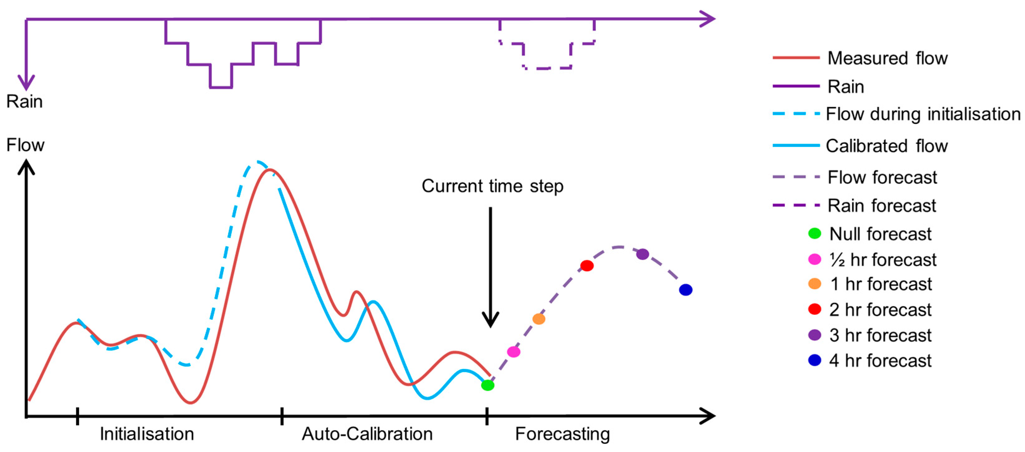
2.1. Online Flow Forecasting Workflow

In this paper, flow forecasts are produced by running a model, which has been calibrated to present conditions. At every point in time where a new forecast is generated, the procedure performs the following three steps: initialisation, auto-calibration and forecasting (see Figure 1). The auto-calibration step is where prior knowledge about the parameters and observed data are incorporated into the model using the MAP method and where a null forecast representing the flow at the present point in time is estimated. During the optimisation, flow is simulated for a period of time that encompasses both the initialisation and the auto-calibration periods but the resulting model fit, produced by every tested set of parameters, is only evaluated with an objective function during the auto-calibration period. The purpose of the initialisation period is thus to generate useful initial conditions for the auto-calibration. The best set of parameters is afterwards applied during the flow forecasting step to produce forecasts up to 4 h into the future. Even short term forecasts of rainfall can be very uncertain and this uncertainty depends upon the forecasting method itself. Observed rainfall was therefore used to generate ex-post flow forecasts (see [29] for a discussion of appropriate modelling terminology). When the model is run into the future, it is thus the actual precipitation that was eventually recorded at that time rather than a meteorological forecast that is used as forcing. This excludes possible errors induced by a specific rainfall forecasting technique during the evaluation of the data assimilation scheme.

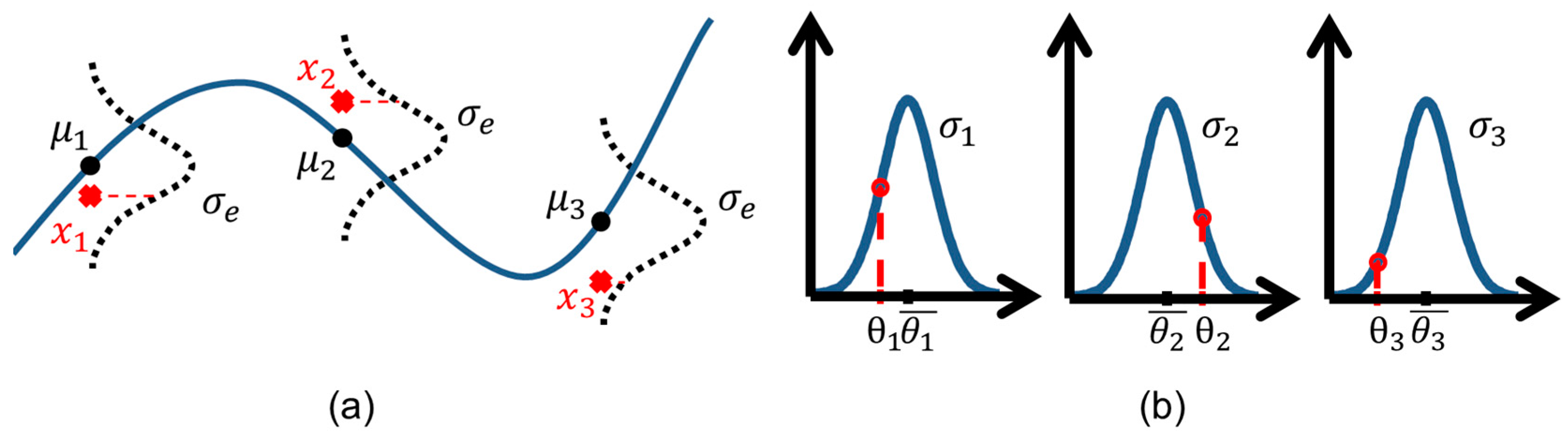
2.2. Data Assimilation with Auto-Calibration of Parameters

The data assimilation method used in this study is based on Maximum a Posteriori estimation (MAP). MAP originates from Bayesian statistics and relies on Bayes’ theorem, given as

$$\mathrm{p}\left(\mathsf{\theta }|x\right)=\frac{\mathrm{p}\left(x\right|\mathsf{\theta }\left)\mathrm{p}\right(\mathsf{\theta })}{\mathrm{p}\left(x\right)}$$

(1)

where $\mathrm{p}\left(\mathsf{\theta }\right)$ is the a priori probability density function (PDF) of the model parameters, $\mathrm{p}\left(x\right)$ is the PDF of the observed data, $\mathrm{p}\left(x\right|\mathsf{\theta })$ is the conditional probability that describes the likelihood of the observation being an outcome of the model, while $\mathrm{p}\left(\mathsf{\theta }\right|x)$ is the a posteriori PDF of the model parameters after the observations have been considered [30]. For simplicity, we assume that the parameters’ PDF can be described by a normal distribution.

Parameter estimation with MAP is here done by locating the set of parameters that produces the mode of the a posteriori PDF, which are seen as the most likely parameter values. Since $\mathrm{p}\left(x\right)$ only serves as a normalising factor [30], and thus does not affect the location of the mode, this estimation procedure can be described as

$${\hat{\mathsf{\theta }}}_{\mathrm{MAP}}={\mathrm{argmax}}_{\mathsf{\theta }} \mathrm{p}(x|\mathsf{\theta })\mathrm{p}(\mathsf{\theta })$$

(2)

MAP simplifies to Maximum Likelihood estimation (ML) if no a priori PDFs are assigned to the model parameters. In the presented approach, the residuals e between model simulations μ_j and observations x_j at time step j during the calibration period are assumed to be uncorrelated and to follow a normal distribution with standard deviation σ_e. The use of these assumptions will be further addressed later in the discussion of this paper. We can then describe $\mathrm{p}\left(x\right|\mathsf{\theta })$ as shown in Equation (3), where N_obs is the number of observation data points in the auto-calibration period.

$$\mathrm{p}\left(x|\mathsf{\theta }\right)={\displaystyle \prod }_{j=1}^{N_{\mathrm{obs}}}\frac{1}{\sqrt{2\mathsf{\pi }}{\mathsf{\sigma }}_e}{\mathrm{e}}^{-\frac{1}{2}{\left(\frac{x_j-{\mathsf{\mu }}_j}{{\mathsf{\sigma }}_e}\right)}^2}$$

(3)

Figure 2a illustrates this relationship between the simulations and the observations. The prior parameter values are assumed normal with mean $\overline{{\mathsf{\theta }}_i}$ and standard deviation ${\mathsf{\sigma }}_i$, which is illustrated in Figure 2b. The prior probability density for the parameter vector $\mathsf{\theta }$ is then found as:

$$\mathrm{p}(\mathsf{\theta })={\displaystyle \prod }_{i=1}^{N_{\mathrm{par}}}\frac{1}{\sqrt{2\mathsf{\pi }}{\mathsf{\sigma }}_i}{\mathrm{e}}^{-\frac{1}{2}{\left(\frac{{\mathsf{\theta }}_i-\overline{{\mathsf{\theta }}_i}}{{\mathsf{\sigma }}_i}\right)}^2}$$

(4)

where N_par is the number of parameters.

2.3. Modelling Tool and Implementation of MAP

The models in this study are set up and auto-calibrated in the generic water modelling tool WaterAspects which is open source software maintained by Krüger A/S-Veolia Water [31].

In WaterAspects, the likelihood function is not maximised as in Equation (2). Instead, the negative log likelihood function is minimised, and Equation (2) becomes

$${\hat{\mathsf{\theta }}}_{\mathrm{MAP}}={\mathrm{argmin}}_{\mathsf{\theta }}-\left(\ln \right(\mathrm{p}\left(x\right|\mathsf{\theta }\left)\right)+\ln \left(\mathrm{p}\right(\mathsf{\theta }\left)\right))$$

(5)

The minimisation of the negative log likelihood function is in WaterAspects done with the iterative Broyden-Fletcher-Goldfarb-Shanno approximation of Newton’s method [32]. The number of iterations that can be performed depends on the available computational power, and the time between the forecasts. After this user-defined timespan, the set of parameters that produces the highest likelihood is selected. The standard deviation σ_e in Equation (3) is estimated based on the model fit at the previous point in time. A good fit results in a low σ_e and vice versa.

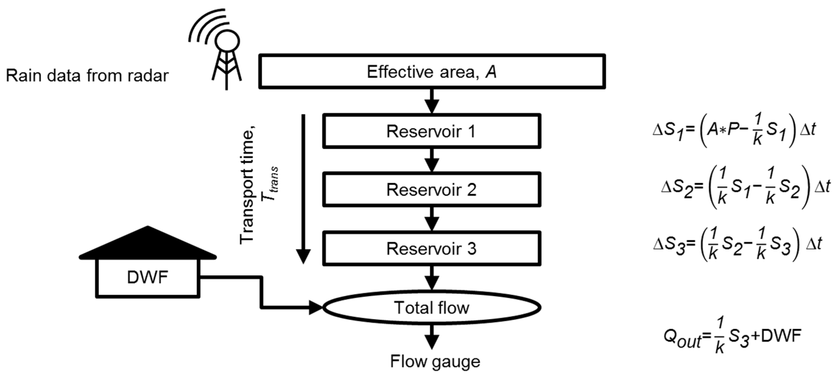
2.4. Modelling Approach

Combined urban drainage systems collect both sewage and stormwater runoff from urban areas which means that the runoff is a mixture of polluted sewage water as well as the runoff induced by rainfall.

While the sewage contributes with pollutants, it is intense rainfall events that cause the system capacity to be exceeded, and it is therefore important to be able to model the rainfall-runoff relationship. Impervious surfaces such as roads and roofs produce runoff that will go straight to the drainage system and result in a fast direct response. On the other hand, rain that falls on pervious surfaces such as lawns and parks will ideally percolate down though the soil and not be intercepted by the drainage system at all. Pervious surfaces can however produce surface runoff in cases where the rainfall intensity exceeds the infiltration capacity or after long wet periods that have led to saturation of the soil. Such conditions can dramatically increase the runoff volume. The physical state of the pipe system will also affect the rainfall-runoff relationship as cracks can lead to significant amounts of infiltration-inflow. As the infiltration in addition is governed by the nature of the soil matrix, it is difficult (if not impossible) to produce reliable deterministic models for areas where the direct response from impervious areas does not dominate the total rainfall response.

In this study, a lumped linear reservoir model (e.g., [33]) is used to emulate the relationship between rainfall and runoff in a given catchment area. The outflow from the reservoir cascade is combined with a dry weather flow (DWF) component, which models the behaviour of the sewage fraction of the total flow in the system, as shown graphically and with equations in Figure 3. The linear reservoir cascade model contains two parameters: an effective runoff area A, and a mean transport time T_trans. The effective area describes the part of the catchment that contributes to runoff and thus determines the volume of the runoff, while the transport time is the average time it takes for runoff to flow through the system and thus governs the shape of the hydrograph. An increase in the effective area leads to a larger volume of runoff, while an increase in the transport time attenuates the response. The single series of reservoirs with a single set of parameters will have to account for various aspects, such as fast and slow runoff components.

DWF originates from the uses of water by households, commercial interests, industry as well as water that infiltrates into pipes [34], and varies both during the day and over the course of the year. Generally, a diurnal pattern appears every day, which in this study is imitated by a sinusoidal function as seen in Equation (6).

$$\mathrm{DWF}={\mu }_{DWF}+{\alpha }_1\sin (2\mathsf{\pi }T+{\omega }_1)+{\alpha }_2\sin (4\mathsf{\pi }T+{\omega }_2)$$

(6)

Here, μ_DWF is the mean of the DWF, α_i and ω_i controls the amplitude, controls the frequency and $T$ is the time of day expressed as a variable that goes from 0 to 1 every 24 h. μ_DWF is included in the auto-calibration to allow for seasonal changes in the dry weather flow, imitating slowly changing infiltration/inflow processes. The other parameters in Equation (6) are kept constant for the sake of simplicity and parameter identifiability.

Three parameters will thus be continuously auto-calibrated: A, T_trans, and μ_DWF Figure 3 illustrates how all three parameters relate to the model setup along with the governing equations for the reservoir series.

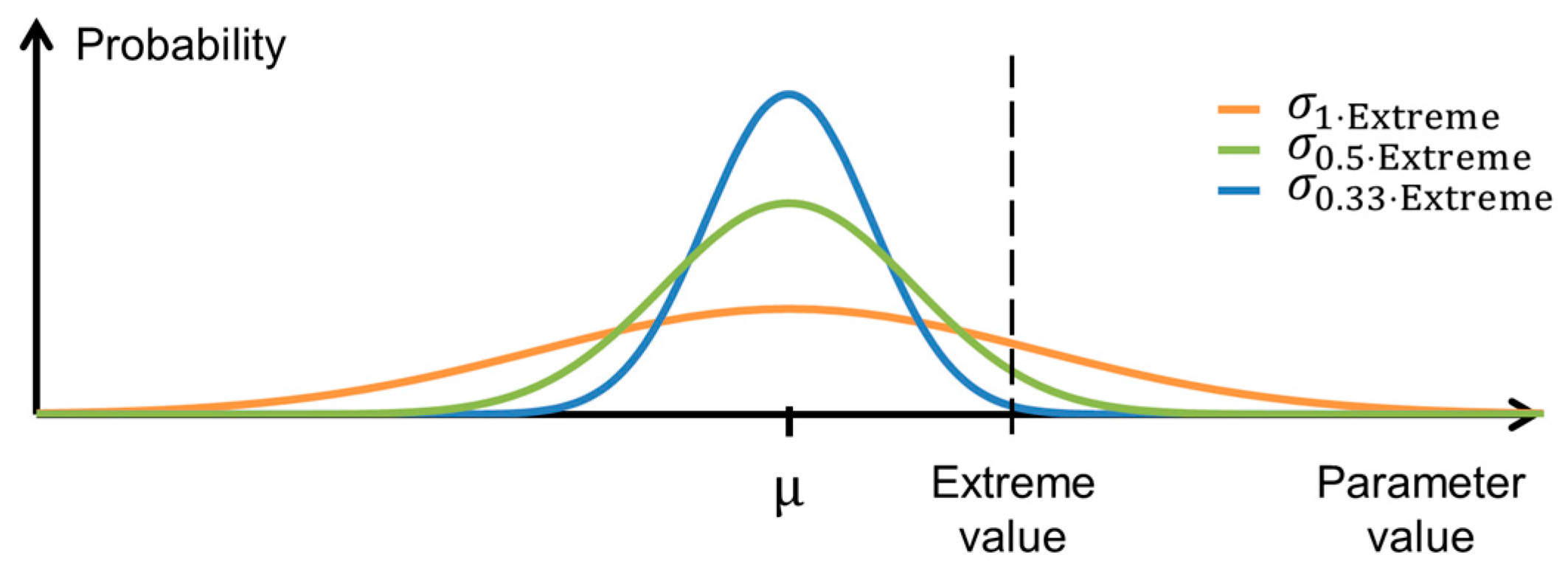
2.5. Setup of the MAP Auto-Calibration

In order to perform the MAP auto-calibration, it is necessary to assign a prior PDF to each of the parameters of the model. In real life applications, the mean values will typically be estimated by ordinary model calibration on a historical time series and the standard deviations will reflect the trust in the estimated parameters and their variation from one event to another. Independent historical time series were not available in this case study and the mean values and standard deviations were therefore determined on the same data series that was used for validation.

The parameters in Equation (6) were determined by performing a ML calibration on a dry period in the middle of the considered data set. Hereafter, the mean A and mean T_trans were determined by a ML calibration on the entire period, and the variability of A and T_trans in the dataset was assessed by estimating them for each individual rain event. The parameter sets obtained through calibration to individual rain events provided an idea of the variations of A and T_trans in the examined catchment. The largest parameter values were seen as an estimate of the extent of the parameter variations and were thus used to evaluate the standard deviations of the a priori distributions, as described in Equation (7).

$$\mathsf{\sigma }=\frac{x-\mu }{z}$$

(7)

Here, $x$ is the most extreme parameter value, $\mu$ is the mean, and $z$ is the standard score, which describes how many standard deviations an observation is larger than the mean. The standard score was set to 1, 2 and 3, resulting in three sets of standard deviations that represent scenarios where the standard deviations are equal to x − μ, half the size of the x − μ and one third of x − μ, respectively. These three sets will later be used to explore how the prior parameter variability affects the considered MAP technique, and will hereafter be referred to as ${\mathsf{\sigma }}_{1\cdot Extreme}$, ${\mathsf{\sigma }}_{0.5\cdot Extreme}$ and ${\mathsf{\sigma }}_{0.33\cdot Extreme}$. Figure 4 illustrates how the three scenarios relate to each other. The parameter means and standard deviations together define the prior PDFs and were kept constant at every point in time.

The length of the auto-calibration period determines how much of the immediate past that is used for updating the model parameters at each time of forecast. If a very long auto-calibration period is used, extreme parameter values will be averaged out and the priors assigned to the parameters will become less important; MAP estimation thus turns into ML as the length of the auto-calibration period increases [35]. If a short auto-calibration period is used, the response of the model will be dominated by very few data points, which will increase the risk of over-fitting the model unless constrained by the priors. Because of this, it is difficult to generally identify an optimal length of the auto-calibration period. However, as a general rule, the length of the period should be longer than the hydraulic response time of the system, ensuring that all effects of a rain event are considered. Three different auto-calibration periods will be investigated in this study, such that the importance of the length of the period to the MAP technique is examined.

2.6. Evaluation of Forecasting Performance

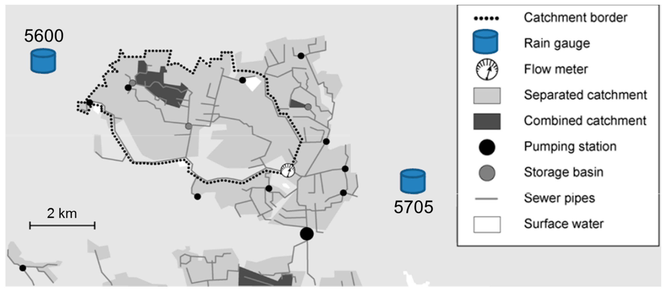
Nine auto-calibrated forecast models combining the three sets of standard deviations for the prior parameter distributions and the three auto-calibration periods are evaluated using the Nash-Sutcliffe efficiency (NSE). In addition, a simulation model without continuous auto-calibration is evaluated, fixing the parameters at the mean values from the prior distributions. These values were calibrated on the same time series that is later used for validation.

3. Case Study

The considered catchment is situated in Ballerup outside of Copenhagen, Denmark. It has a total area of 1300 ha and an area-velocity flow meter is located downstream of the catchment as seen in Figure 5. The area is part of a larger complex catchment area connected to the wastewater treatment plant in Avedøre, and is already well known from several research studies [36,37,38,39,40]. The drainage system is known to have problems with infiltrating water, which causes the hydraulic response of the system to be very different from wet to dry periods of the year, a phenomenon that is very difficult to model deterministically (see the explanations in Section 2.4).

Rain data was obtained as the areal average of rain estimated by a C-band radar, which is situated in Stevns approximately 45 km south of the catchment and operated by the Danish Meteorological Institute. The radar has been adjusted by using a total of seven rain gauges from the Danish SVK network [41] such that the average deviations between the cumulated rainfall observed by the rain gauges and the radar are minimised during the data period (the specific procedure is described in [38,42]). Amongst these gauges, gauge 5600 and 5705 (shown in Figure 5) are located closest to the Ballerup catchment. The considered time period in this study is two months from 1 July 2010 to 31 August 2010, which was a very rainy period that was preceded by a dry period.

4. Results and Discussion

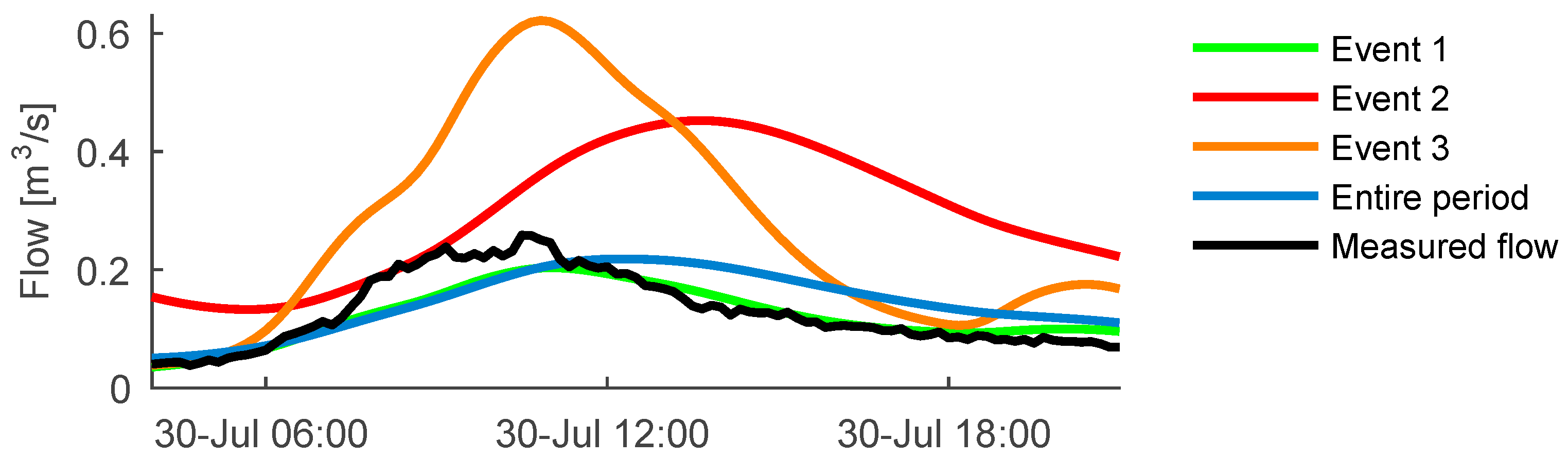
4.1. Prior Parameter Distributions, DWF Equation and Choice of Auto-Calibration Periods

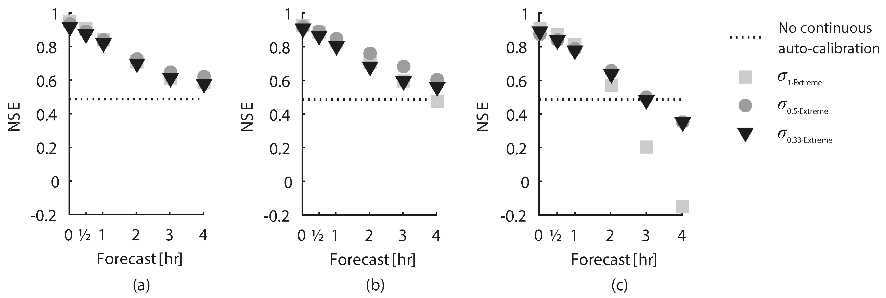
First, the mean of the prior μ_DWF distribution and the shape parameters in Equation (6) were obtained without any constraints on the parameter ranges during the ML calibration on a dry weather period. This resulted in a DWF model that was used during the calibration of the mean values for the effective area and transport time. A and T_trans were calibrated on the entire data set with the same ML procedure (see

Table 1. Estimates of the constant DWF shape parameters as well as the mean and standard deviation of the three variable model parameters.

Parameter	Unit	Mean Value	Mean Value Calibrated on	Standard Deviation
				${\mathsf{\sigma }}_{1\cdot \mathit{Extreme}}$	${\mathsf{\sigma }}_{0.5\cdot \mathit{Extreme}}$	${\mathsf{\sigma }}_{0.33\cdot \mathit{Extreme}}$
α1	m3/s	−0.0322	A dry weather period
α2	m3/s	−0.0165
ω1	—	1.17
ω2	—	−0.0391
μDWF	m3/s	0.074		0.029	0.015	0.0097
A	m2	113,125	The entire dataset	280,721	140,361	93,574
Ttrans	h	9.36		6.54	3.27	2.18

).

To provide an overview of how much the catchment parameters vary from the mean values during various events, the area and transport time were calibrated for numerous single rain events with a constant dry weather flow model (μ_DWF, α_i and ω_i). This is illustrated in Figure 6 where the parameters calibrated from three distinct events are applied to simulate a completely different rain event. This clarifies how deficits in the model structure and rainfall input lead to very different parameter values from event to event, such that parameters calibrated for single events cannot simply be extrapolated to others. The most extreme calibrated parameter values for a single event are an effective area of 393,846 m² and a transport time of 15.9 h. The most extreme value for μ_DWF is 0.103 m³/s and is obtained by calibration on a dry weather period at the very end of the data set, which is preceded by a very wet period. These extreme parameter values were used to derive the three standard deviation scenarios via the expression in Equation (7). The three standard deviations for each of the three variable model parameters are given in Table 1.

In this study, initial runs showed that using auto-calibration periods in the same order of magnitude as the transport time gave good results. As the transport time is event specific, and there are issues with both too short and too long auto-calibration periods, an optimal length of the period will never be obtained. Therefore, the mean and the most extreme transport times of 9.36 and 15.9 h, respectively, were used as guidelines and led to the selection of three auto-calibration periods of 8, 12 and 16 h for the following discussion.

4.2. Effects of Applying Different $\sigma$-Scenarios and Different Lengths of Auto-Calibration Period

The effects on the overall model performance of applying the different σ-scenarios and auto-calibration periods are shown in Figure 7, which compares NSE values for 0–4 h forecasts based on all the observations in the data set. Note that the model performance without data assimilation is a horizontal line due to the fact that observed rainfall data is used as forecasted rainfall and therefore the length of the forecast horizon has no impact on the results. The addition of data assimilation clearly results in overall better forecasts than the simulation model without data assimilation, with the exception of 3–4 h forecasts with models that have a 16 h auto-calibration period.

Generally, forecast performance decreases as the forecast horizon increases for all combinations of σ-scenarios and auto-calibrations periods. This happens because the model parameters are calibrated to present conditions, which become less representative the further into the future a forecast is made. The least constrained parameter scenario, ${\mathsf{\sigma }}_{1\cdot Extreme}$, produces the best forecasts for 0–½ h while the ${\mathsf{\sigma }}_{0.5\cdot Extreme}$-scenario performs best for the 1–4 h forecasts. This indicates that the parameters in the most variable scenario are over-tuned to present conditions and thus not suitable for extrapolation further into the future.

The best 0–½ h forecasts have an auto-calibration period of 8 h while the best 1–3 h forecasts have one of 12 h. This suggests that the near future is better represented by the near past while the longer forecasts are represented better by parameters calibrated over a longer time period. It is, however, worth noting that the 4 h forecast is best for the 8 h auto-calibration period. This, and the fact that forecasts with a 16 h auto-calibration period perform worse than the shorter calibration periods, illustrates the need for catchment specific considerations by the user during setup.

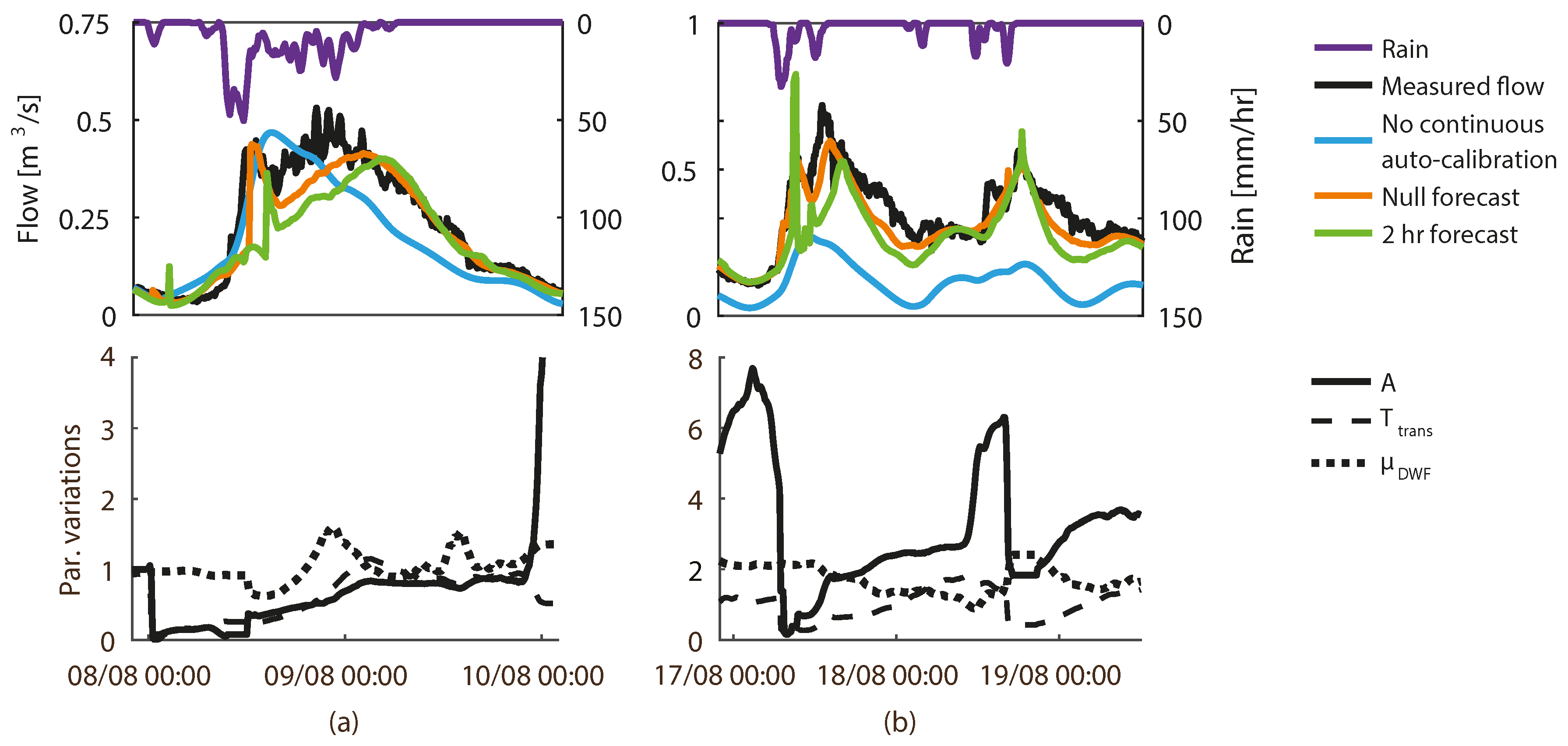
4.3. Visual Representation of Forecast Abilities and Parameter Variations

In this section, 2 h flow forecasts are given for two selected events in order to visualise how auto-calibration with MAP produces flow forecasts through continuous changes in the underlying model parameters. The provided examples are from the ${\mathsf{\sigma }}_{0.5\cdot Extreme}$-scenario with an auto-calibration period of 12 h, which produced the best 2 h forecasts as seen in Figure 8. In the Figure, the “Null forecast” denotes the modelled flow that is produced by the calibrated parameter set at each time step. “No continuous auto-calibration” represents the modelled flow that is produced by keeping the parameters constant at their respective mean values.

A rain event in early August 2010 is shown in Figure 8a. Dry weather conditions were present prior to the considered event, which is why both of the wet weather parameters, A and T_trans, start at their mean values. In the beginning of the event, a small amount of rain is observed without a corresponding increase in runoff. Therefore, the auto-calibration reduces A and T_trans to near-zero in order to prevent that the first small amounts of rain affect the modelled flow. This results in an underestimation of the entire rising limb of the subsequent hydrograph as the low A and T_trans values cause a delay in the forecasted response. The error is not corrected before increasing flow observations are assimilated into the model, leading to an increase in A. The model does not forecast the measured flow well until the end of the rain event where a steady increase in A and T_trans magnifies both the storage and detention of water in the system, thus capturing the long tail of the hydrograph. In comparison, the model without data assimilation cannot capture the tail of the hydrograph, but it is worth noting that the constant parameters produce a better fit in the beginning of the event. This shows that excessive parameter variations in this case reduce the method’s forecast-ability. Figure 8b illustrates a rain event later in August 2010. This event follows several days of rain, which leads to a value of A about seven times higher than the expected mean value at the beginning of the event. The large A results in an overestimation in the forecasted flow at first, which is corrected by a sudden decrease in A. This decrease to near-zero, and a similar decrease of T_trans, afterwards leads to the same kind of delay in the response and underestimation that was seen in Figure 8a. The hydrograph’s tail is also underestimated, despite the increase in A and T_trans. This underestimation, which is also seen on the tail of the second peak in Figure 8b, is most likely due to either heavy soil saturation in the catchment produced by consecutive days of rain and/or dynamics of a storage reservoir in the drainage system. Neither of these aspects are described explicitly in the simple model structure. The model without data assimilation underestimates the flow significantly throughout this event primarily because it is unable to increase the μ_DWF in the same way that the auto-calibrated model is.

4.4. Benefits and Challenges When Using MAP for Auto-Calibration

Comparing the parameter variations in Figure 8 reveals that the parameters, especially A, can vary a lot in order to make the simple model fit the complex reality. The variations span from near-zero to several times the expected mean value. These low and high values have low probability in the prior PDFs but are still chosen in the MAP estimation. This could be because short auto-calibration periods can lead to unstable parameters. On the other hand, increasing the length of the auto-calibration period will lead to more stable parameter estimates but also diminishes the desired effect of including prior parameter distributions.

Breinholt et al. [37] examined parameter variations in a similar, yet slightly more complex, linear reservoir model used for simulation of flow in the same case study area. They found that it is very difficult to estimate prior distributions related to wet weather parameters (which in this study are A and T_trans). Many different parameter sets performed well, which indicated a problem with model equifinality and potential insensitivity to model performance or mutual correlation of the various parameters. The linear reservoir model applied in this study is a very simple conceptualization of reality and, hence, many complex features of urban hydrology are lumped into the three parameters. A discrepancy between the model and measurements can arise from issues with the model structure, poor model states, errors in the rainfall forcing data etc. All of these aspects will be compensated for through direct updates to the model parameters in this type of scheme. This also makes it difficult to determine the three parameters’ “true” distributions. Normal a priori distributions were assumed for the three parameters for the sake of simplicity and the standard deviations were used to investigate the influence of a priori parameter variability on the forecasting ability of this simple yet practical method. In the future, a broader evaluation on the type of probability distribution in relation to each parameter could be interesting.

Formal statistical approaches to data assimilation based on Bayesian theory, such as MAP estimation, rely on assumptions related to the model residuals. Examples of these assumptions relate to auto-correlation and the specific probability distribution of the residuals, and these assumptions are often hard to justify theoretically in hydrological modelling applications (we refer to [43] for a detailed discussion on the relationship between explanatory depth and power, as well as the usefulness of predictive models with limited realism). An assumption of the presented MAP estimation is that consecutive deviations between observed and modelled values are independent. This is clearly not true for this case and the estimation approach, described by Figure 3 and Figure 4, essentially corresponds to a least squares based output error method. We have not considered schemes that account for the correlation between model residuals because the focus of this work is on the effect of parameter updating on forecast performance for a method that is currently used in practice. In addition, Breinholt et al. [16] have demonstrated in the same catchment that the output error method yields models with strong simulation performance. Furthermore, the residuals from the auto-calibration period at each time step were assumed to be normally distributed during the parameter estimation. These residuals are not expected to actually be normally distributed due to the simple model structure, but the normal assumption was here used for practical reasons.

It should also be noted that the method is affected by the quality of the rain input where a time displacement, e.g., caused by the use of rain gauges, can result in the same type of erratic parameter variability seen in the examples. If rain is observed without an equivalent increase in observed runoff, this technique will decrease the parameters related to the amount of water that is in the model, which might later lead to a delayed response in the forecast. If an increase in runoff is observed without an equivalent increase in observed rainfall then this technique will increase the parameters related to the amount of water that is in the model, which might later lead to an overestimation in the forecasts. The basic issue with a MAP scheme of this type is thus that the parameters are varied only after the errors have occurred. Time displacements in the model input will, however, also negatively affect other data assimilation methods that update model states as documented in [44]. Observed rainfall is used to generate the ex-post flow forecasts in this study, which excludes the uncertainty related to actual rainfall forecasting. Errors in the rainfall forecasts will translate into the flow forecasts and could potentially reduce the positive effects of the corrections made during the auto-calibration procedure. Examining the effect of using actual radar rainfall forecasts in ex-ante flow forecasting with MAP is considered beyond the scope of this paper as the result is bound to be highly dependent on the specific rainfall forecasting technique. It is, however, an important factor during operational use and would be an interesting topic for future studies.

The necessary simple model structures for real-time operations will also affect the parameter variability. In the examined case, the large variations in A and T_trans between individual rain events suggest that incorporating slow and fast runoff as two separate regimes could improve results. This has previously been shown to be the case for simulation models and stochastic grey-box models for the same case study area [16,37]. A somewhat more complex model structure would of course increase the predictive performance but not eliminate the necessity of updating the model entirely. It would be interesting to compare the performance of the presented MAP data assimilation techniques with other techniques based e.g., on state updating. By updating the states of the model, the short term forecast would surely be better, since the state variable in the most downstream reservoir in this case would be adjusted much more directly to the observed flow. It is, however, rarely the very short term forecasts that are the most important for forecasting and control purposes, and since state updating in itself will not adjust the model parameters to changing conditions, the longer forecasts might be deteriorated compared to the proposed method. The outcome of such a comparison is bound to be case-dependent since both the quality of the model and rain data, as well as the extent of shifts and trends in the hydrological system that is modelled will play a role.

4.5. Guidance for Practical Implementation

Experiences from practical operation of this scheme with radar-based rainfall forecasts as input [26] have shown that it is important not to underestimate the combined time needed for initialisation and auto-calibration. Underestimating this time can lead to a deficit in the amount of surface runoff in the model compared to what is being measured, which will be the case if the precipitation that causes runoff occurred before the considered period. The combined time that the initialisation period and auto-calibration period cover should therefore be at least as long as the longest observable response times in the system. If the system contains storage basins, the combined time should be longer than the time it takes to empty the largest basin. Failing to do so can cause unstable parameter variations and potentially unwanted changes to the dry weather flow component as compensation.

Setting standard deviations for each parameter is a case dependent matter. Operational experiences have shown that 10% of the calibrated mean parameter values is a good starting point. From here, manual evaluation can improve the performance further. For case areas where large parameter variation is a recurring issue, it has in practice been useful to set hard limits on the variability.

The primary use of this method, as it is currently being operated at various locations in Denmark, is for switching of wastewater treatment plants into wet weather operation mode before large amounts of runoff enter the plants. Thus, avoidance of underestimating flow for small to medium size rain events is of higher concern than overestimation of flow for large rain storms. It can also be advantageous to discriminate between dry weather and wet weather situations in the way the approach is set up. This has especially been useful when detention basins in the system are emptied during dry weather situations. Here, such discrimination allows for keeping the effective area and transport time parameters constant, which mitigates any unwanted adjustments before the next rain event occurs. Finally, flow prediction with the considered flow forecasting approach has generally been more successful for frontal precipitation systems than sudden convective storms. During these storms, it may be worth considering the use of constant wet weather parameters.

5. Conclusions

In the current study, the use of Maximum a Posteriori (MAP) based auto-calibration as a data assimilation tool for urban rainfall runoff models was described in theory and illustrated in a case study. The benefit of using MAP based auto-calibration is that prior knowledge about model parameters is continuously weighed against the model fit to incoming flow observations in real time. The main purpose was to document, evaluate and discuss a methodology already used in practice from both a practical and theoretical viewpoint.

Selecting an appropriate length of the auto-calibration period is a very important part of the MAP auto-calibration method presented here. There is a risk of not accounting for relevant rain inputs if the period is too short. Furthermore, a short length can lead to the model being over-fitted to present conditions. On the other hand, the effect of the prior distributions of the parameters diminishes as the auto-calibration period is increased. For very long auto-calibration periods, stable parameter estimates would be obtained as the method converges to a least squares estimation. However, the model would no longer update to new observations.

By selecting different combinations of prior distributions and auto-calibration periods, it was for the studied catchment noted that the least constrained parameter scenario (${\mathsf{\sigma }}_{1\cdot Extreme}$) was over-tuned to present conditions. An auto-calibration period of 12 h gave better 1–3 h forecasts while the shorter period of 8 h was more adequate for the shorter forecasts. However, the best performing combinations of prior distribution width and auto-calibration period changed from one event to another. The method is thus not straightforward and requires manual tuning when used by practitioners.

Two forecast examples were given in order to visually evaluate the method. Updating of the mean dry weather flow seemed to adapt the model to slow changing flow components in a stable manner, which generally increases the forecast performance. Updating the area and travel time parameters however often leads to erratic parameter changes and time-delayed forecasts. This illustrates a conceptual problem of the method as forecast errors need to be observed before parameters can be updated.

There are some notable benefits to the method that can make it relevant for future implementation. It is easy to implement and understand for anyone who has worked with auto-calibration methods and it is computationally efficient. It generally improves the forecast performance compared with a simulation model without data assimilation, and the time series of parameter variations also provide valuable information about how the system behaviour changes over time.

This study was performed on a two month period and a longer time period could be used for additional evaluation of the MAP approach. Further improvements of the approach may include automatically tuning the auto-calibration setup by estimating the prior standard deviations and auto-calibration period in such a way that the forecast error is minimised. Another approach would be to update the prior distributions continuously instead of keeping them constant as in this study.

References

1. Grum, M.; Thornberg, D.; Christensen, M.L.; Shididi, S.A.; Thirsing, C. Full-scale real time control demonstration project in Copenhagen’s largest urban drainage catchments. In Proceedings of the 12th International Conference on Urban Drainage, Porto Alegre, Brazil, 11–16 September 2011.
2. Fradet, O.; Pleau, M.; Marcoux, C. Reducing CSOs and giving the river back to the public: Innovative combined sewer overflow control and riverbanks restoration of the St. Charles River in Quebec City. Water Sci. Technol. 2011, 63, 331–338. [Google Scholar] [CrossRef] [PubMed]
3. Pabst, M.; Alex, J.; Beier, M.; Niclas, C.; Ogurek, M.; Peikert, D.; Schütze, M. ADESBA—A new general global control system applied to the Hildesheim sewage system. In Proceedings of the 12th International Conference on Urban Drainage, Porto Alegre, Brazil, 11–16 September 2011.
4. Puig, V.; Cembrano, G.; Romera, J.; Quevedo, J.; Aznar, B.; Ramón, G.; Cabot, J. Predictive optimal control of sewer networks using CORAL tool: Application to Riera Blanca catchment in Barcelona. Water Sci. Technol. 2009, 60, 869–878. [Google Scholar] [CrossRef] [PubMed]
5. Seggelke, K.; Löwe, R.; Beeneken, T.; Fuchs, L. Implementation of an integrated real-time control system of sewer system and waste water treatment plant in the city of Wilhelmshaven. Urban Water J. 2013, 10, 330–341. [Google Scholar] [CrossRef]
6. Harremoës, P.; Madsen, H. Fiction and reality in the modelling world-Balance between simplicity and complexity, calibration and identifiability, verification and falsification. Water Sci. Technol. 1999, 39, 1–8. [Google Scholar] [CrossRef]
7. Schilling, W.; Fuchs, L. Errors in stormwater modeling—A quantitative assessment. J. Hydraul. Eng. 1986, 112, 111–123. [Google Scholar] [CrossRef]
8. Schellart, A.N.A.; Liguori, S.; Krämer, S.; Saul, A.J.; Rico-Ramirez, M.A. Comparing quantitative precipitation forecast methods for prediction of sewer flows in a small urban area. Hydrol. Sci. J. 2014, 59, 1418–1436. [Google Scholar] [CrossRef]
9. Liguori, S.; Rico-Ramirez, M.A.; Schellart, A.N.A.; Saul, A.J. Using probabilistic radar rainfall nowcasts and NWP forecasts for flow prediction in urban catchments. Atmos. Res. 2012, 103, 80–95. [Google Scholar] [CrossRef]
10. Rico-Ramirez, M.A.; Liguori, S.; Schellart, A.N.A. Quantifying radar rainfall uncertainties in urban drainage flow modelling. J. Hydrol. 2015, 528, 17–28. [Google Scholar] [CrossRef]
11. Hutton, C.J.; Vamvakeridou-Lyroudia, L.S.; Kapelan, Z.; Savic, D.A. Real-Time Modelling and Data Assimilation Techniques for Improving the Accuracy of Model Predictions: Scientific Report. Available online: https://emps.exeter.ac.uk/media/universityofexeter/emps/research/cws/downloads/PREPARED_Deliverable_3_6_2_Final.pdf (accessed on 30 August 2016).
12. Hutton, C.J.; Kapelan, Z.; Vamvakeridou-Lyroudia, L.S.; Savic, D.A. Real-time data assimilation in urban rainfall-runoff models. Procedia Eng. 2014, 70, 843–852. [Google Scholar] [CrossRef] [Green Version]
13. Liu, Y.; Weerts, A.; Clark, M.P.; Hendricks Franssen, H.J.; Kumar, S.; Moradkhani, H.; Seo, D.J.; Schwanenberg, D.; Smith, P.J.; Van Dijk, A.I.J.M.; et al. Advancing data assimilation in operational hydrologic forecasting: Progresses, challenges, and emerging opportunities. Hydrol. Earth Syst. Sci. 2012, 16, 3863–3887. [Google Scholar] [CrossRef]
14. Hansen, L.S.; Borup, M.; Møller, A.; Mikkelsen, P.S. Flow forecasting using deterministic updating of water levels in distributed hydrodynamic urban drainage models. Water 2014, 6, 2195–2211. [Google Scholar] [CrossRef] [Green Version]
15. Ho, J.Y.; Lee, K.T. Grey forecast rainfall with flow updating algorithm for real-time flood forecasting. Water 2015, 7, 1840–1865. [Google Scholar] [CrossRef]
16. Breinholt, A.; Møller, J.K.; Madsen, H.; Mikkelsen, P.S. A formal statistical approach to representing uncertainty in rainfall-runoff modelling with focus on residual analysis and probabilistic output evaluation—Distinguishing simulation and prediction. J. Hydrol. 2012, 472–473, 36–52. [Google Scholar] [CrossRef]
17. Borup, M.; Grum, M.; Madsen, H.; Mikkelsen, P.S. A Partial Ensemble Kalman Filtering approach to enable use of range limited observations. Stoch. Environ. Res. Risk Assess. 2015, 29, 119–129. [Google Scholar] [CrossRef] [Green Version]
18. Vrugt, J.A.; Gupta, H.V.; Nualláin, B.; Bouten, W. Real-Time Data Assimilation for Operational Ensemble Streamflow Forecasting. J. HydRometeorol. 2006, 7, 548–565. [Google Scholar] [CrossRef]
19. Madsen, H.; Skotner, C. Adaptive state updating in real-time river flow forecasting—A combined filtering and error forecasting procedure. J. Hydrol. 2005, 308, 302–312. [Google Scholar] [CrossRef]
20. Shamseldin, A.Y.; O’Connor, K.M. A non-linear neural network technique for updating of river flow forecasts. Hydrol. Earth Syst. Sci. 2001, 5, 577–598. [Google Scholar] [CrossRef]
21. Moradkhani, H.; Sorooshian, S.; Gupta, H.V.; Houser, P.R. Dual state-parameter estimation of hydrological models using ensemble Kalman filter. Adv. Water Resour. 2005, 28, 135–147. [Google Scholar] [CrossRef]
22. Dumedah, G.; Coulibaly, P. Evaluating forecasting performance for data assimilation methods: The ensemble Kalman filter, the particle filter, and the evolutionary-based assimilation. Adv. Water Resour. 2013, 60, 47–63. [Google Scholar] [CrossRef]
23. Todini, E. Rainfall-Runoff Models for Real-Time Forecasting. In Encyclopedia of Hydrological Sciences; John Wiley & Sons, Inc.: New York, NY, USA, 2005; pp. 1869–1896. [Google Scholar]
24. Kowalsky, M.B.; Finsterle, S.; Rubin, Y. Estimating flow parameter distributions using ground-penetrating radar and hydrological measurements during transient flow in the vadose zone. Adv. Water Resour. 2004, 27, 583–599. [Google Scholar] [CrossRef]
25. Hsu, K.L.; Moradkhani, H.; Sorooshian, S. A sequential Bayesian approach for hydrologic model selection and prediction. Water Resour. Res. 2009, 45. [Google Scholar] [CrossRef]
26. Thorndahl, S.; Poulsen, T.S.; Bøvith, T.; Borup, M.; Ahm, M.; Nielsen, J.E.; Grum, M.; Rasmussen, M.R.; Gill, R.; Mikkelsen, P.S. Comparison of short-term rainfall forecasts for model based flow prediction in urban drainage systems. Water Sci. Technol. 2013, 68, 472–478. [Google Scholar] [CrossRef] [PubMed]
27. Thorndahl, S.; Rasmussen, M.R. Short-term forecasting of urban storm water runoff in real-time using extrapolated radar rainfall data. J. Hydroinform. 2013, 15, 897–912. [Google Scholar] [CrossRef]
28. Lund, N.S.V.; Pedersen, J.W.; Borup, M.; Grum, M.; Mikkelsen, P.S. Auto-calibration for data assimilation in linear reservoir models used in flow forecasting of urban runoff. In Proceedings of the 13th International Conference on Urban Drainage, Kuching, Sarawak, Malaysia, 7–12 September 2014.
29. Beven, K.; Young, P. A guide to good practice in modeling semantics for authors and referees. Water Resour. Res. 2013, 49, 5092–5098. [Google Scholar] [CrossRef] [Green Version]
30. Bernardo, J.M.; Smith, A.F.M. Bayesian Theory; John Wiley & Sons, Inc.: New York, NY, USA, 2008. [Google Scholar]
31. Grum, M.; Longin, E.; Linde, J.J. A flexible and extensible open source tool for urban drainage modelling: www.WaterAspects.org. In Proceedings of the 6th International Conference on Urban Drainage Modelling, Dresden, Germany, 15–17 September 2004.
32. Fletcher, R. Practical Methods of Optimization, 2nd ed.; John Wiley & Sons, Inc.: New York, NY, USA, 1987. [Google Scholar]
33. Chow, V.T.; Maidment, D.R.; Mays, L.W. Applied Hydrology; McGraw-Hill, Inc.: New York, NY, USA, 1988. [Google Scholar]
34. Butler, D.; Davies, J.W. Urban Drainage, 3rd ed.; Spon Press: London, UK, 2011; pp. 215–218. [Google Scholar]
35. Velickov, S. Nonlinear Dynamics and Chaos with Applications to Hydrodynamics and Hydrological Modelling; CRC Press: Leiden, The Netherlands, 2004. [Google Scholar]
36. Borup, M.; Grum, M.; Mikkelsen, P.S. Real time adjustment of slow changing flow components in distributed urban runoff models. In Proceedings of the 12th International Conference on Urban Drainage, Porte Allegre, Brazil, 11–16 September 2011.
37. Breinholt, A.; Grum, M.; Madsen, H.; Thordarson, F.Ö.; Mikkelsen, P.S. Informal uncertainty analysis (GLUE) of continuous flow simulation in a hybrid sewer system with infiltration inflow—Consistency of containment ratios in calibration and validation? Hydrol. Earth Syst. Sci. 2013, 17, 4159–4176. [Google Scholar] [CrossRef]
38. Löwe, R.; Thorndahl, S.; Mikkelsen, P.S.; Rasmussen, M.R.; Madsen, H. Probabilistic online runoff forecasting for urban catchments using inputs from rain gauges as well as statically and dynamically adjusted weather radar. J. Hydrol. 2014, 512, 397–407. [Google Scholar] [CrossRef]
39. Löwe, R.; Mikkelsen, P.S.; Madsen, H. Stochastic rainfall-runoff forecasting: Parameter estimation, multi-step prediction, and evaluation of overflow risk. Stoch. Environ. Res. Risk Assess. 2014, 28, 505–516. [Google Scholar] [CrossRef] [Green Version]
40. Del Giudice, D.; Löwe, R.; Madsen, H.; Mikkelsen, P.S.; Rieckermann, J. Comparing two stochastic techniques for reliable urban runoff predictions by modeling systematic errors. Water Resour. Res. 2015, 51, 5004–5022. [Google Scholar] [CrossRef]
41. Jørgensen, H.K.; Rosenørn, S.; Madsen, H.; Mikkelsen, P.S. Quality control of rain data used for urban runoff systems. Water Sci. Technol. 1998, 37, 113–120. [Google Scholar] [CrossRef]
42. Thorndahl, S.; Rasmussen, M.R.; Neve, S.; Poulsen, T.S.; Grum, M. Vejrradarbaseret Styring af Spildevandsanlæg; DCE Technical Report 95; Aalborg University: Aalborg, Denmark, 2010. [Google Scholar]
43. Beven, K. A philosophical diversion. In Environmental Modelling: An Uncertain Future? An Introduction to Techniques for Uncertainty Estimation in Environmental Prediction; Routledge: London, UK, 2009; pp. 31–48. [Google Scholar]
44. Borup, M.; Grum, M.; Mikkelsen, P.S. Comparing the impact of time displaced and biased precipitation estimates for on-line updated urban runoff models. Water Sci. Technol. 2012, 68, 109–116. [Google Scholar] [CrossRef] [PubMed]
Figure 1. Illustration of the three steps that constitute the applied flow forecasting procedure; modelled flow is shown for the initialisation, the auto-calibration and the forecasting steps.
Water 08 00381 g001
Figure 2. Depiction of Maximum a Posteriori estimation; (a) How likely the observations are to be an outcome of the model, p ( x | θ ) ; (b) Total a priori parameter probability, p ( θ ) , for a model with three parameters.
Water 08 00381 g002
Figure 3. The setup of the cascading linear reservoir model with Ttrans = 3/k, which also takes DWF into account. Here, S refers to the reservoir storage, P to precipitation intensity, Qout to simulated flow at the outlet and Δt to the time step in the model.
Water 08 00381 g003
Figure 4. Visualisation of the connection between extreme parameter values and applied standard deviations.
Water 08 00381 g004
Figure 5. Ballerup catchment (Edited from [37]).
Water 08 00381 g005
Figure 6. Observed flow for an example event compared to simulations performed with four different model calibrations: three single event calibrations and a calibration using the entire data period.
Water 08 00381 g006
Figure 7. Forecast performance for different σ-scenarios with a fixed length of the auto-calibration period; (a) 8 h; (b) 12 h; (c) 16 h.
Water 08 00381 g007
Figure 8. Example of two rain events modelled with the σ 0.5 E x t r e m e -scenario and an auto-calibration period of 12 h. (Upper) Measured flow together with the null forecast and the 2 h forecast. (Lower) Variations of parameters relative to their estimated mean values (cf. Table 1). (a) Rain event from 8 to 10 August (b) Rain event from 17 to 19 August.
Water 08 00381 g008