Socio-Ecological Regionalization of the Urban Sub-Basins in Mexico

Abstract

Mexico is a diverse country in terms of culture and natural environments. For this reason, the delimitation of homogeneous basins with similar environmental, social, and economic attributes is important in order to facilitate the elaboration of high-impact regional development strategies. However, this represents an ongoing challenge due to the complexity of the interactions that occur within socio-ecological systems at a regional scale. In the present study, the main objective was to identify the interrelationships among different aspects of the socio-ecological system located within basins, with the goal of utilizing this information to promote the region-specific sustainable development of an Integrated Water Resources Management (IWRM). Therefore, in this study, environmental, social, economic, and institutional variables, relevant to water management and with the capacity to be expressed spatially, were utilized to identify regions with similar characteristics and to regionalize the urban sub-basins of Mexico based on a principal component analysis (PCA) and the k-medoids clustering algorithm. The identification of the most adequate number of regions at the national level was determined by the silhouette method. As a result, five distinct regions for Mexico were generated, which forms the first step in the design of integrated water resources management strategies for these regions.

1. Introduction

The development of water management strategies at regional, national, and local levels is key for guiding the adequate use of water resources [1]. Integrated Water Resources Management (IWRM) is a paradigm for governing water management and is part of a multidimensional systematic process, where the sustainable development and use of water resources is achieved through the integration of the involved environmental, economic, social, and institutional subsystems. This process recognizes the interactions among sectors that ultimately lead to the adequate use or abuse of water resources and thus seeks to address fundamental environmental concerns [2]. In addition, this focus has far-reaching implications, as key information from each of the analyzed subsystems is taken into consideration in addition to system-wide interrelationships.

The sectors that influence water resources management may be conceptualized as forming part of a dynamic system (socio-ecological) of response and feedback loops, where social and ecological processes are linked [3]. For example, an ecosystem may be modified due to the use of its water resources by the surrounding human population, and subsequently, the dependent population provides feedback in light of changes to the water provision capacity of the ecosystem [4]. However, in order to understand water management in Mexico, it is important to recognize that it has been historically based on two counter-opposing models. The traditional model is informed by a centralized and generalized management of resources on behalf of the federal administration of the country. The second model corresponds to a more integrated concept of management, defined by growing means of decentralized management in which official institutions are challenged or backed by groups from civil society that demand an increased public participation in decision making; however, a national database of such social participation does not exist. Although the latter model is the most inclusive and egalitarian, federal organisms such as the National Water Commission (CONAGUA, for its acronym in Spanish) have voluntarily and involuntarily resisted the development and implementation of such measures [4]. Therefore, in Mexico, water management is still largely centralized in regional CONAGUA offices that coordinate and administrate water resources by means of 13 regional Basin Committees (BCs).

Since the beginning of the 21st century, about 80% of the countries on the planet have made changes to their water policies, water laws, and water plans. Of the 27 developed countries, 16 have already fully or partially implemented the IWRM approach. While 38% of 77 developing countries, such as Mexico, have included it in their plans, the level of implementation varies widely [5].

Articles 4 and 27 of the Constitution of the United Mexican States define that “the State shall guarantee the right to access and enjoy water, in which the law must establish the bases and the participation of the three orders of government and the citizenry.” In recent years, regulations, strategies, and activities have been increasingly generated and updated to formulate a national water policy that tackles the country’s various water problems. These new efforts are informed by the IWRM framework and its adoption in Mexico.

The National Water Law (NWL) dictates that each BC address the problems of a defined hydrological administrative region (HAR), formed by a group of basins and sub-basins considered to be the basic units of IWRM. Although in theory this respects some aspects of an IWRM, this delimitation is performed according to political boundaries rather than other defining characteristics in order to facilitate the administration and integration of relevant socioeconomic data also collected within political boundaries [6]. While BCs are indeed supported by local committees and basin councils, including Groundwater Technical Committees (Comités Técnicos de Aguas Subterráneas, COTAS) that are composed of public servants and may include members from independent organizations or civil society, these members do not have a vote in decision making [7].

However, in Mexico, the IWRM model has not yet been fully consolidated in practice [8], although it is formally the guiding axis of water policy. Therefore, this paradigm has already been adopted but is still in the process of being implemented. In this sense, IWRM is experiencing a process of convergence, in which, as Bennet [9] points out, the development of public policies involves at least five aspects: (1) definition of goals; (2) definition of formal content; (3) construction of instruments for the management and assignment of executors; (4) definition of results indicators and consequences of their implementation; and (5) orientation in the formulation of the policy itself (style of politics). To these aspects, Dolowitz and Marsh [10] pointed out that the convergence of ideologies, ideas, attitudes, and concepts should be added.

Thus, the convergence of national water policies based on IWRM represents part of a gradual and incremental process that follows the general ideology of the model. This is evidenced mainly in the 2004 reform of the National Water Law, although this process began much earlier with the decentralization of agricultural irrigation waters. This model was further consolidated with the adoption of management principles at the watershed level and the search (at least written) of greater social participation in decision making regarding water resources [11].

Furthermore, the demand for water in Mexican cities is mainly determined by rapid population growth, water shortages, and increased drought [12]. Thus, managing water resources in urban basins with high population densities and distinct socio-ecological systems represents a challenge. In this scenario, an urban basin may be defined as a basin that partially or completely contains an urban zone [13]. In addition, IWRM recognizes the close and interdependent relationships between urban zones and hydrological basins and aims to identify their characteristics.

Accordingly, this study proposes a socio-ecological regionalization of the urban sub-basins of Mexico, based on variables that were rated by experts as being influential in the sustainability of water resources. The identification of sub-basins with similar characteristics allows for the establishment of water resources planning and management strategies that are responsive to the specific needs of an area.

Regionalization Algorithms

The management of water resources must take into consideration the spatial array of the multidimensional characteristics of a region, as well as their interactions, in order to identify hydrological sub-basins with similar attributes [14]. For these purposes, regionalization techniques function by grouping homogeneous entities, which may provide valuable information to decision makers in numerous disciplines. In this case, multivariate statistical techniques were used to identify regions with similar bioclimatic characteristics [15] in terms of humidity, aridity, and precipitation.

Several of the following techniques form part of the most commonly utilized methods for the regionalization of areas based on their attributes: principal component analysis (PCA), cluster algorithms (fuzzy c-means, k-means, k-medoids, and hierarchical, among others), classification and regression trees (CART) [16,17], or several of these in combination [18,19,20]. Of these, one of the most frequently utilized clustering algorithms is the k-means [21], which sequentially calculates the k centroid of each of the clusters and then assigns each object to the closest centroid. However, this algorithm is sensitive to atypical data among the variables [22]. On the other hand, the k-medoid algorithm uses medoids instead of centroids and has been shown to be more efficient [23], where the medoid is the object of a data set with minimal dissimilarity to all other objects, which determines the cluster. This technique is less vulnerable to atypical data in comparison with the k-means method [24]. Among the k-medoid algorithms, the partitioning around medoids (PAM) method is the most powerful [25,26]. Finally, one of the greatest challenges of regionalization is the determination of the optimal number of regions. For this, different validation methods have been developed, including both external and relative methods. External methods compare output data with a known data structure, while relative methods compare different data inputs and calculate the distance between data objects, simplifying the result in an index (e.g., Davies-Boulding and Silhoutte, among others) [27].

Although there are different methods for regionalization, there are relatively few studies that aim to define entities by using variables of a distinct nature geared toward measuring not only environmental but also socioeconomic or agricultural factors [28]. Consequently, in Mexico, multidimensional regionalization studies that include basin characteristics unrelated to water behavior are scarce, although Monroy-Ortiz [29] notably made an effort to identify urban basins and their main hydrological characteristics. However, it is still necessary to relate regionalization techniques with diverse variables based on economic, environmental, social, and institutional aspects that would allow for sub-basins with similar characteristics located at distinct regions of the country to be determined, thus offering support for more focused and efficient regional planning and decision making within an IWRM framework.

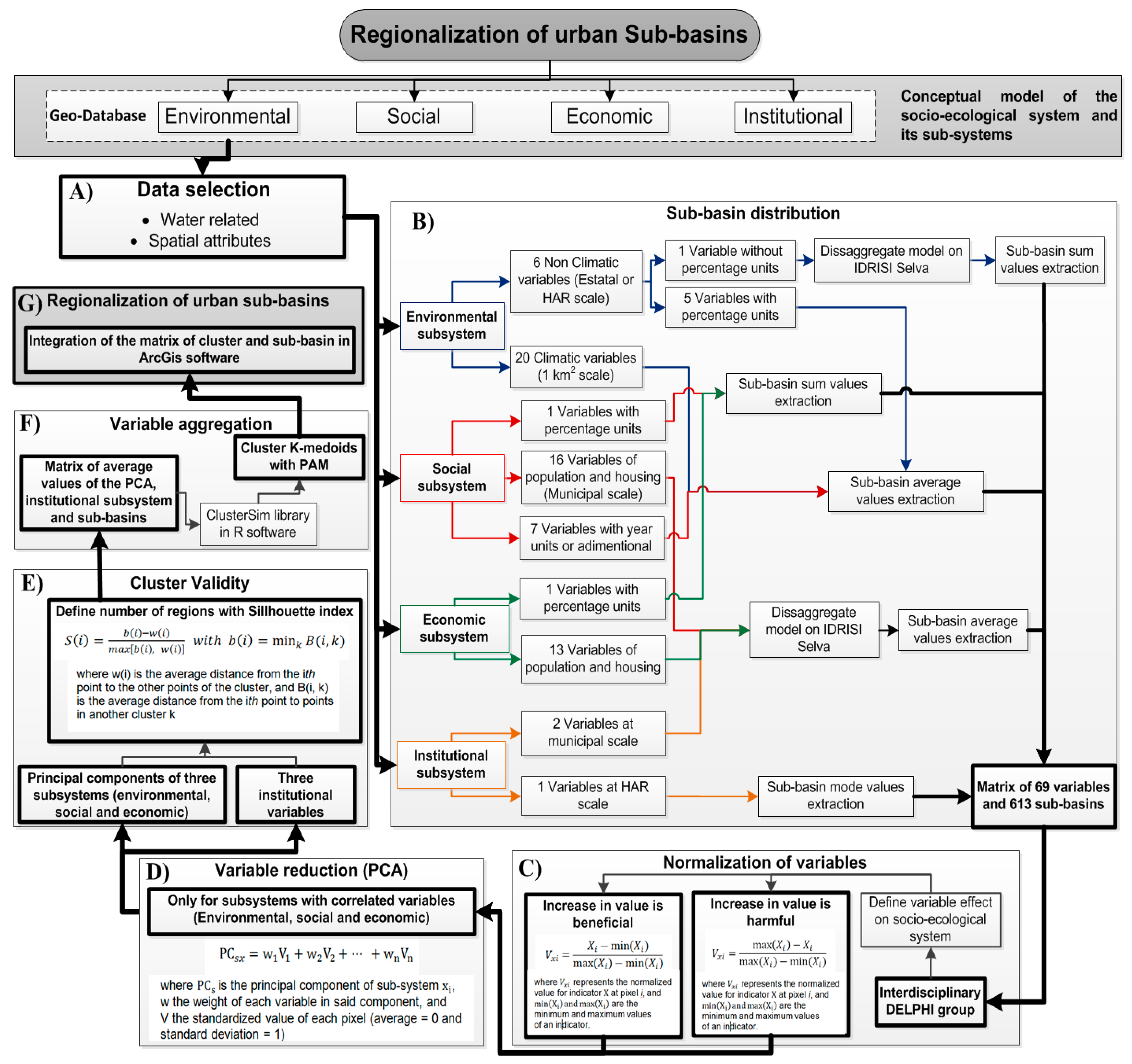
2. Materials and Methods

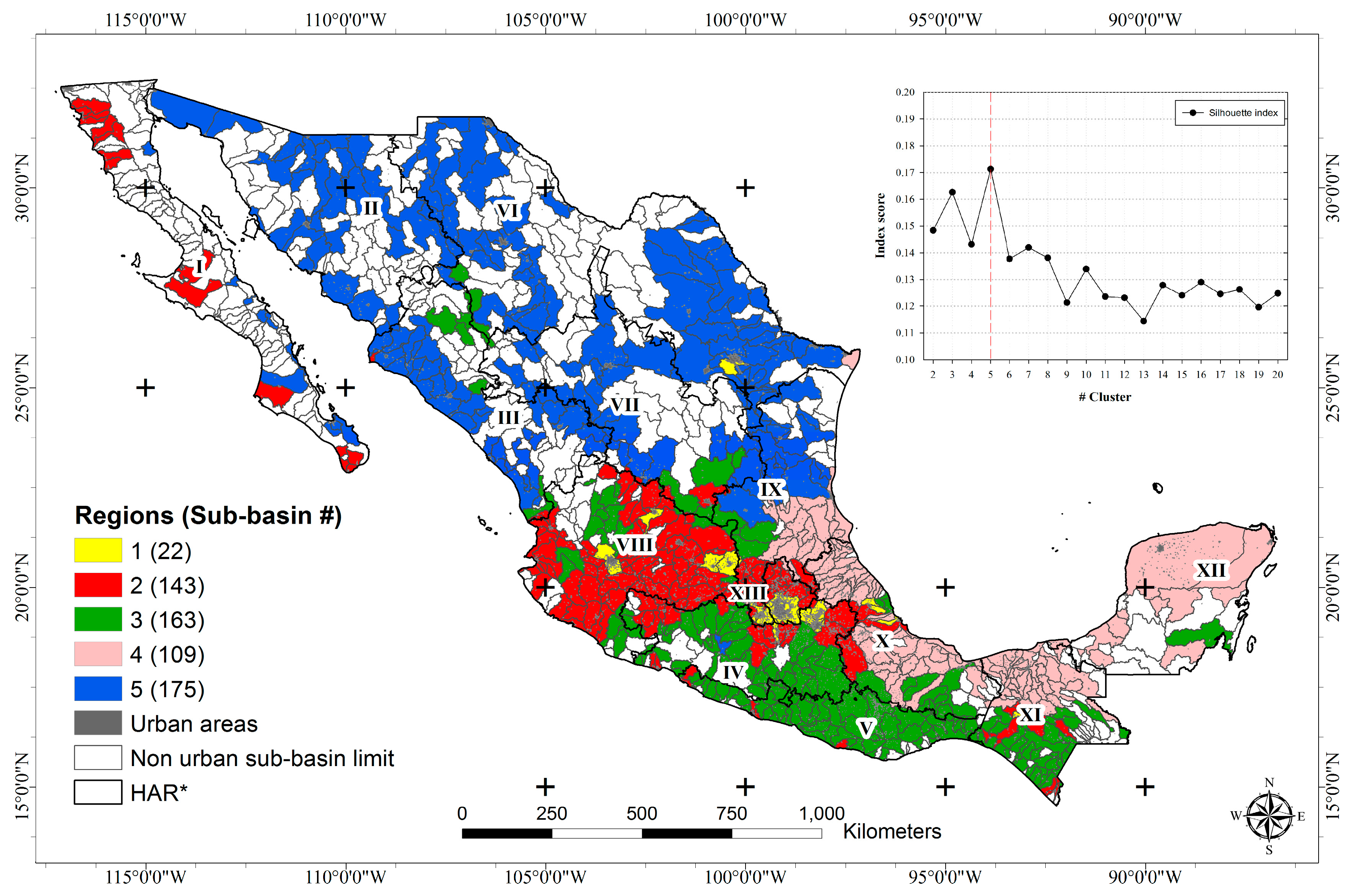
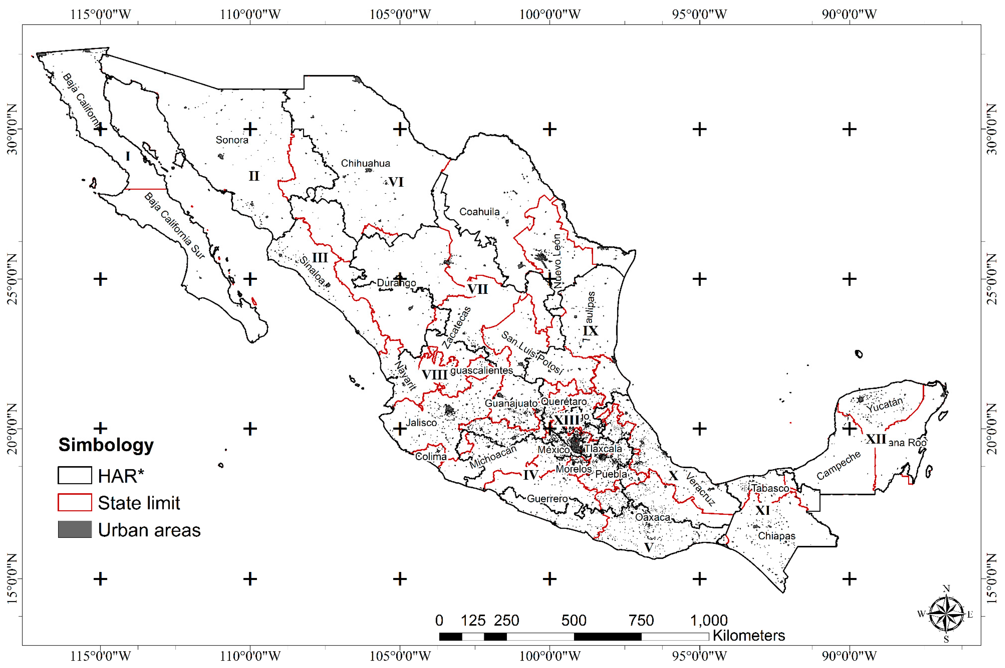
2.1. Study Area

As the Tropic of Cancer passes through the midsection of Mexico, the geographic position of the country enables the presence of both temperate and tropical zones. The country also has extensive coastlines and is surrounded by the Pacific Ocean, the Gulf of California, the Gulf of Mexico, and the Caribbean Sea. Moreover, its diverse topography is the product of a turbulent geological history, and mountain ranges extend from the North to the South and from the East to the West along the Trans-Mexican Volcanic Belt [30]. Such characteristics enable Mexico to have nearly all of the world’s existing climate types, except extreme cold [31], along with their corresponding ecosystems and biological species, including many species that are endemic to Mexico [32]. Thus, Mexico may be considered a megadiverse country.

The northern region of the country is largely arid or semi-arid, representing 56% of the land area and characterized by an annual rainfall level of less than 500 mm. Meanwhile, the climate of the southeast portion of the country is humid and has an annual rainfall level of greater than 2000 mm [33]. Accordingly, the country has a wide variety of geological and physiographic characteristics and both endorheic and exorheic basins, resulting in diverse conditions that are relevant for the IWRM. Due to its geographic location, Mexico is regularly exposed to severe hydrometeorological events such as hurricanes and intense rainfall that, while increasing the availability of surface water and the natural recharge of aquifers, also cause damage to the population, infrastructure, services, and productive systems [34].

In order to administrate and regulate the use of surface and ground waters in Mexico, the country was divided into 13 HARs, each with a regional center managed by CONAGUA, the federal organism recognized by the NWL as holding jurisdiction in hydrological management [35]. Within the HARs, 731 hydrological basins and 974 sub-basins are contained.

Politically, the country is composed of 31 sovereign states subdivided in municipalities, including a federal district subdivided in delegations that is the seat of the federal powers of the nation [36]. Together, these areas span a continental surface area of 1.9 million km² (Figure 1). Following the criteria of National Institute of Geography and Statistics (INEGI, for its acronym in Spanish), areas designated as urban have a population of greater than 2500 inhabitants, while areas with fewer inhabitants are considered rural. In this context, 78% of the total population of 112,336,538 inhabitants lives in urban centers [37].

As Mexico in this sense is largely an urban country, urban areas are currently considered to be the most active territorial component and likewise a motor of economic growth and social development. The tendency toward the concentration of the population and economic activities in cities is due to the greater opportunities for wealth creation, investment, employment, and creation of products and services with added value, which are factors that translate to economic and social well-being [38]. One example of the advances in infrastructure and social well-being is that in Mexico, in comparison with other countries of Latin America, there is an extensive network of water infrastructure and high coverage of services, running water, and wastewater treatment. In addition, CONAGUA subsidizes up to 70% of the cost of modernizing public works projects for public drainage systems in cities of more than 50,000 inhabitants [39].

Economic planning is centralized in the metropolitan area of Mexico City (MAMC), which is considered to be the epicenter of the national economy, as it generates around 32% of the gross domestic product (GDP). Correspondingly, cities close to the MAMC, such as Queretaro, Toluca, Puebla, Guadalajara, and Aguascalientes, have also experienced a large economic and industrial impulse [40]. However, these centers of economic and population growth are also located in areas with a relatively dry climate, in contrast with the southeastern region of the country that contains 72% of water runoff but only economically contributes 16% of the national GDP [39]. Meanwhile, in the northern part of the country, the increase in economic agreements with the United States has led to a rapid growth in population and economic activity (GDP: 33.3%), leading to increased urbanization and investments in infrastructure for the treatment and provision of water [41].

In Mexico, the area supplied by surface water corresponds to 38% of the continental surface, which means that more than 60% of the territory needs groundwater supply systems. In addition, as a result of problems related to water management deficiencies and the unsustainable management of water resources, 104 of the 731 hydrological basins present problems of water availability [34]. The supply of sufficient amounts and quality of water for human consumption is one of the basic demands of the population, as it has a direct impact on their health and overall well-being. This is also recognized by the guiding instruments of national planning: the National Development Plan 2013–2018 [42] and the National Water Program 2014–2018 [34].

The largest volume of water concessions for consumptive uses, are provided for the agricultural sector, mainly for irrigation (76.6%), and for the urban public supply (14.2%). These two water uses are supplied with an approximate volume of 30,000 Hm³ of groundwater and 47,000 Hm³ of surface water [43]. CONAGUA considers 95.5% of urban areas and 80.3% of rural areas to be covered by the public water supply or to be able to obtain water from a nearby dwelling [43]. Furthermore, 96.5% of urban areas and 70.1% of rural areas are connected with wastewater infrastructure, including connections to the sewer network, a septic tank, a drain, canyon, lake, or the sea [44].

The evaluation of surface water quality in Mexico is carried out using three indicators: biochemical oxygen demand (BOD₅), chemical oxygen demand (COD), and total suspended solids (TSS). Sites with continuous water quality monitoring are located in areas with high anthropogenic influence. According to these three indicators (BOD₅, COD, and TSS), the water was determined to be highly contaminated at 187 sites out of 5000 in the country, in at least two of or all of the indicators [43]. Sampling sites classified as contaminated have increased in number since 2012 in terms of COD parameters (26.2% of sampled sites) and TSS (4.7% of sampled sites) compared with data sampled in 2015 (COD 40.2% and TSS 4.9%) [44].

Furthermore, overexploitation of aquifers and surface water in Mexico is more alarming every year: 32 aquifers were overexploited in 1975 and 106 in 2013. Alongside the exhaustive use of water, in many places additional problems such as deforestation have contributed to decreasing aquifer recharge. In cities, green areas have been increasingly replaced by paved areas that prevent adequate infiltration, among other problems [34].

2.2. Selection of Variables

Integrated Water Resources Management should have management strategies that adapt to areas with similar characteristics in order to maximize invested resources; this strategy is even more critical considering the heterogeneous conditions of the territory. To identify homogeneous basins within the socio-ecological system, databases from environmental, social, economic, and institutional subsystems were selected. From these, key variables considered to influence water resources management within urban sub-basins that had the capacity to be expressed spatially were selected (Figure 2A), from the reference year of 2010 or in its absence, from 2005. Data for climatic variables [45] were represented as the average values for each selected variable over the 1950–2000 period. The data was expressed spatially per km², and average values were extracted for each urban sub-basin of the country. The treatment, management, and territorial interpretation of the data extracted from the databases was carried out in the Idrisi Selva (Clark Labs, Worcester, MA, USA) [46] and ArcMap 10.2 (ESRI, Redlands, CA, USA) [47] geographic information systems.

As the spatial data and scales (municipal, state, HAR) for some of the variables were distinct or presented in vector format, for these cases, the average values per urban sub-basin were also extracted. Variables expressed at the municipal level were transformed to density per km² and distributed at the sub-basin level. This re-distribution was constructed using the disaggregate model in the Idrisi Selva software (Clark Labs) [48], which uses municipal densities and statistically distributes them by taking into consideration the distance between the sub-basin limits and the centroids of an urban area (Figure 2B).

2.3. Normalization of Variables

The Delphi group analysis technique is a multidisciplinary participation technique useful for IWRM and is based on expert opinions. It allows for a structured and interactive communication between groups of people, permitting knowledge to be shared across sectors in order to resolve a complex problem [49]. Based on this technique, several expert reunions were carried out at the Interamerican Center of Water Resources (Centro Interamericano de Recursos de Agua, CIRA) in order to arrive at a consensus on the effect of different socio-ecological variables and whether their increase or decrease was beneficial or harmful for water resources management, or, in other words, to verify if positive values resulted in a beneficial effect on water resources, or, complementarily, if an increase in a variable’s value has a harmful effect, using the equations in Tan et al. [50] (Figure 2C).

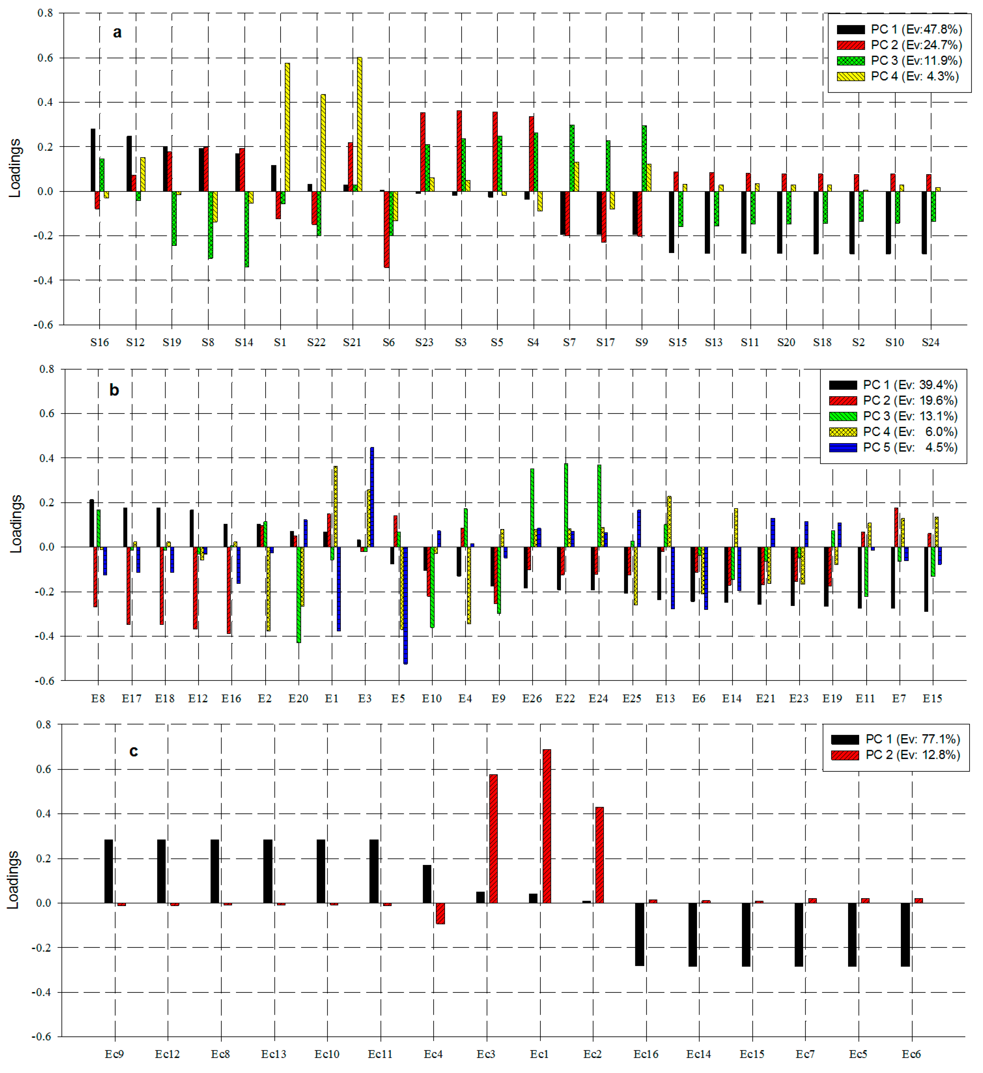
2.4. Reduction of Variables

With the objective of reducing the dataset to represent only the most relevant information for the spatial analysis, a PCA of the normalized variables of each subsystem was carried out in order to remove the highly correlated variables and thus reduce the number of explanatory variables. The PCAs were calculated in the Statgraphics Centurion V 15.2 software (Statpoint Technologies, Warrenton, VA, USA) [51] for the environmental, social, and economic subsystems. For the institutional subsystem, this technique was not performed due to the nature of its variables (this subsystem only has three), which were unable to be correlated. Principal components with eigenvalues equal to or greater than one were selected [52]. This was carried out with the goal of reducing the group of correlated variables and expressing them along the most simplified dimension [53] (Figure 2D).

2.5. Regionalization and Validation of the Cluster Analysis

With the principal components obtained for the environmental, social, and economic subsystems and the three variables of the institutional component, the k-medoids cluster method was applied using the PAM (partitioning around medoids) algorithm. The number of regions was not subjective but rather defined by the silhouette (S) index, which was used to measure and validate the consistency of the regionalization and to determine the number of adequate regions given the utilized variables [27]. According to Rosseeuw [54], S measures the relationship between clusters based on the distance between them and the average value of the distances, where coefficient values closer to 1 indicate more differentiated clusters [55] (Figure 2E).

The integration of S with the k-medoids analysis was carried out in the R statistical software v.3.1.0 [56], using the ClusterSim library. The process was performed using the matrix of average values of the principal components per sub-basin, where two groups were selected as a minimum and 20 as a maximum (Figure 2F). Finally, the matrix of sub-basins groups was integrated to a spatial map using ArcMap 10.2 [47] geographic information system (Figure 2G).

3. Results and Discussion

The urban sub-basins of Mexico covered 62.9% of the national territory (613 sub-basins). The remaining percentage was composed of non-urban sub-basins with population centers of less than 2500 inhabitants. The latter are mainly found in the northern region of the country, which is characterized by conditions of aridity and, in general, extreme climates [31]. It is likely that these conditions inhibit the establishment and development of large urban centers.

Eight databases were considered (

Table A1. Geo-databases used for variable selection.

Database	Sustainability Subsystem	Spatial Resolution	Variables Selected
National Institute of Statistics and Geography (Instituto Nacional de Estadística y Geografía [INEGI]) [37]	Social	1 km	1
National System of Municipal Information (Sistema Nacional de Información Municipal [SNIM]) [62]	Social, Economic	Municipal	21, 16
Average disability-adjusted life years (DALYs) due to intestinal disease (DALYs) and mean natural water availability [63]	Social	1 km	2
National Water Commission (Comisión Nacional del Agua (CONAGUA) [6]	Institutional	HAR *	1
Mexican Business Information System (Sistema de Información Empresarial Mexicano [SIEM]) [64]	Institutional	Municipal	1
National Association of Universities and Higher Education Institutions in Mexico (Asociación Nacional de Universidades e Instituciones de Educación Superior en México [ANUIES]) [65]	Institutional	Municipal	1
Worldclim [45]	Environmental	1 km	20
Secretariat of the Environment and Natural Resources, National System of Environmental Indicators (Secretaría de Medio Ambiente y Recursos Naturales, Sistema Nacional de Indicadores Ambientales [SNIA-SEMARNAT]) [66]	Environmental	State, HAR *	6
* Hydrological-Administrative Region	Total		69

, Appendix A), from which a matrix of 613 urban sub-basins was constructed with 69 descriptive variables related to the use and management of water. The matrix contained 26 variables in the environmental subsystem, 24 in the social, 16 in the economic, and three in the institutional (Table A1, Appendix A). In

Table B1. Variables used for regionalization of urban sub-basins. Beneficial (+) or harmful (−) effect on water resources management.

Subsystem	Source	ID	Variable	Units/km2 of Sub-Basin	Range of Values		Effect	Description
					Min	Max
Environmental	SNIA-SEMARNAT	E1	Soil degradation	%	4.3	73.2	−	Soil degradation caused by humans
		E2	Wastewater treatment plant efficiency	%	29.4	98.3	+	Ratio between treatment capacity of treatment plant and actual volume of treated wastewater
		E3	Disinfected water supply	L/inhab/day	0.0	235.3	+	Volume of disinfected water supply
		E4	Biochemical Oxygen Demand (indicator of contamination)	%	0.0	23.9	−	Average annual BOD values range from 30 to 120 mg/L
		E5	Biochemical Oxygen Demand (indicator of high levels of contamination)	%	0.0	51.9	−	Average annual BOD values higher than 120 mg/L
		E6	Intensity of groundwater use	%	1.3	133.9	−	Ratio between extraction volume and natural recharge of aquifer
	WORLDCLIM	E7	Average annual minimum temperature (Tmin)	°C	2.4	22.9	+	Period average, 1950–2000
		E8	Average annual maximum temperature (Tmax)	°C	18.4	36.0	−	Period average, 1950–2000
		E9	Temperature seasonality	%	6.3	76.6	−	Standard deviation of temperature
		E10	Isothermality	%	33.2	81.2	+	Ratio of mean diurnal range to annual range
		E11	Mean temperature of the coldest month	°C	4.3	27.6	+	Period average, 1950–2000
		E12	Mean temperature of the warmest month	°C	13.2	31.3	−	Period average, 1950–2000
		E13	Mean diurnal range in temperature	°C	5.9	19.8	−	Monthly average multiplied by the difference between monthly Tmax and Tmin
		E14	Annual range in temperature	°C	11.4	38.6	−	Difference between Tmax of warmest month and Tmin of coldest month
		E15	Tmin of the coldest month	°C	0.0	20.5	+	Period average, 1950–2000
		E16	Tmax of the warmest month	°C	21.0	39.9	−	Period average, 1950–2000
		E17	Mean temperature of the wettest quarter	°C	9.2	31.3	−	Average of three wettest months of the year
		E18	Mean temperature of the driest quarter	°C	9.2	31.3	−	Average of three driest months of the year
		E19	Average annual precipitation	mm	52.2	3681.5	+	Period average, 1950–2000
		E20	Precipitation seasonality	%	44.4	125.8	+	Precipitation coefficient of variation
		E21	Precipitation level of the wettest quarter	mm	39.4	1663.7	+	Average of three wettest months of the year
		E22	Precipitation level of the driest quarter	mm	0.9	394.2	+	Average of three driest months of the year
		E23	Precipitation level of the wettest month	mm	16.4	610.5	+	Period average, 1950–2000
		E24	Precipitation level of the driest month	mm	0.0	118.6	+	Period average, 1950–2000
		E25	Precipitation level of the warmest quarter	mm	14.8	1044.5	+	Average of three warmest months of the year
		E26	Precipitation level of the coldest quarter	mm	5.9	730.4	+	Average of three coldest months of the year
Social	INEGI	S1	Proportion of urban land use per sub-basin	%	0.1	57.3	−	Percentage of sub-basin occupied by urban areas (more than 2500 inhabitants)
	SNIM	S2	Population attending school	Inhabitant	0.3	997.9	+	Population older than 3 years attending school
		S3	Education level of female population	Year	3.3	10.8	−	Average years of schooling of female population
		S4	Education level of male population	Year	3.9	10.9	+	Average years of schooling of male population
		S5	Overall education level	Year	3.7	10.8	+	Average years of schooling of population
		S6	Population density	Inhabitant	0.3	3633.4	−	Number of inhabitants per km2
		S7	Human Development Index (HDI)	Range 0–1	0.3	0.8	+	Human Development Index
		S8	Marginalization index	Range 0–100	7.4	60.9	−	Marginalization index
		S9	Population that speaks an indigenous language	Inhabitant	0.0	90.2	+	Number of inhabitants (≥3 years) that speak an indigenous language
		S10	Male population that speaks an indigenous language	Inhabitant	0.0	44.6	+	Number of male inhabitants (≥3 years) that speak an indigenous language
		S11	Female population that speaks an indigenous language	Inhabitant	0.0	45.7	+	Number of female inhabitants (≥3 years) that speak an indigenous language
		S12	Density of inhabited houses	House	0.3	972.0	−	Total number of inhabited houses
		S13	Houses with running water	House	0.3	923.0	+	Number of inhabited houses with running water
		S14	Houses without running water	House	0.0	34.2	−	Number of inhabited houses without running water
		S15	Houses with drainage service	House	0.1	937.4	+	Total number of inhabited houses connected to the drainage network or a septic tank
		S16	Houses without drainage service	House	0.0	32.2	−	Total number of inhabited houses without drainage
		S17	Houses with water, drainage, and electricity	House	0.1	906.1	+	Number of inhabited houses with running water, drainage, and electricity
		S18	Houses with basic goods	House	0.0	968.6	+	Number of inhabited houses with television, radio, refrigerator, washer, automobile, phone, cell phone, computer, and internet
		S19	Houses without basic goods	House	0.0	9.0	−	Number of inhabited houses without television, radio, refrigerator, washer, automobile, phone, cell phone, computer, and internet
		S20	Houses with electricity	House	0.3	944.6	+	Number of inhabited houses with electricity
		S21	Houses without electricity	House	0.0	3.3	−	Number of inhabited houses without electricity
		S22	Houses with sanitary facilities	House	0.3	939.7	+	Number of inhabited houses with toilet or sanitary facilities
	GOMEZ-ALBORES (2012) [63]	S23	Average disability-adjusted life years (DALYs) due to intestinal disease	Rate/10,000 inhab	0.1	77.4	−	Life years lost due to intestinal diseases
		S24	Average natural water availability	m3/year	0.0	2,541,539.7	+	Mean natural water availability per capita
Economic	SNIM	Ec1	Overall economic participation rate	%	31.8	63.3	+	Ratio of working population to overall population with capacity to work (≥15 years)
		Ec2	Male economic participation rate	%	45.4	82.8	+	Ratio of male working population to overall population with capacity to work (≥15 years)
		Ec3	Female economic participation rate	%	6.6	45.2	+	Ratio of female working population to overall population with capacity to work (≥15 years)
		Ec4	Gross domestic product (GDP)	$	0.0	514,410.2	+	Gross domestic product per capita at the municipal level
		Ec5	Overall economically inactive population	Inhabitant	0.1	1248.1	−	Population that is pensioned or retired, including students, homemakers, and those that have a permanent physical or mental impairment that prevents them from working (≥12 years)
		Ec6	Economically inactive male population	Inhabitant	0.0	362.9	−	Economically inactive male population
		Ec7	Economically inactive female population	Inhabitant	0.1	885.2	−	Economically inactive female population
		Ec8	Overall economically active population	Inhabitant	0.1	1588.0	+	Population with a job, or looked for a job in the reference week (≥12 years)
		Ec9	Economically active male population	Inhabitant	0.1	983.1	+	Economically active male population
		Ec10	Economically active female population	Inhabitant	0.0	605.0	+	Economically active female population
		Ec11	Overall economically active and with a job	Inhabitant	0.3	1518.9	+	Population that had a job in the reference week (≥12 years)
		Ec12	Economically active male population with a job	Inhabitant	0.1	927.8	+	Economically active male population with a job
		Ec13	Economically active female population with a job	Inhabitant	0.0	582.4	+	Economically active female population with a job
		Ec14	Overall economically active population without a job	Inhabitant	0.0	77.9	−	Number of inhabitants who did not work or hold a job but looked for work in the previous week (≥12 years)
		Ec15	Economically active male population without a job	Inhabitant	0.0	55.3	−	Male population economically active without a job
		Ec16	Economically active female population without a job	Inhabitant	0.0	22.6	−	Female population economically active without a job
Institutional	ANUIES	I1	Higher education institutions	Institution	0.0	0.2	+	Number of higher education institutions registered in ANUIES
	SIEM	I2	Business density	Businesses	0.0	32.9	−	Number of businesses registered in the Mexican Business Information System
	CONAGUA	I3	Total water management organizations	Committees	2.0	18.0	+	Number of councils, commissions, basin committees, and groundwater committees per HAR

(Appendix B), the positive or negative effects for the IWRM of urban sub-basins are listed, as determined by the interdisciplinary group of experts and the Delphi group analysis technique.

For the environmental, social, and economic subsystems, the corresponding variables were correlated and reduced to principal components (PCs) with the objective of eliminating the variables correlated among them and decreasing the number of explanatory variables. For the institutional subsystem, a PCA was not performed, as two of the three variables were not correlated (p < 0.05). Thus, the PCs were linearly composed of the variables and their resulting weights, where the weights of the variables reflected their contribution to the analysis (Figure 3).

In the social subsystem, the PCs explained 88.7% of the variance (Figure 3a). The first PC was positively explained by the density of inhabited private houses (IPH) without drainage (S16) and negatively correlated with average natural water availability per capita (S24). The second PC was positively related to overall education level (S5) and negatively to population density (S6). The third PC was positively explained by the Human Development Index (S7) and was negatively correlated with the number of IPH without running water (S14). Finally, the fourth PC was positively explained by the density of IPH without electricity (S21) and the percentage of urbanized area within the sub-basin (S1), in addition to being negatively correlated with the marginalization index (S8).

In the environmental subsystem, 26 variables were analyzed and summarized in five principal components that explained 82.6% of variance (Figure 3b). The variable with the highest positive weight in PC 1 was the average annual maximum temperature (E8), and the most negative was the minimum temperature of the coldest month of the year (E15). Along PC 2, the average annual minimum temperature (E7) had the highest positive weight, and the most negative was the maximum temperature of the warmest month (E16). The third PC was positively explained by precipitation levels during the driest quarter of the year (E22) and negatively by the seasonality in precipitation (E20). The fourth and fifth PC contributed 10.2% of the variance and were positively explained by the proportion of soil degradation (E1) and the disinfected water supply per inhabitant (E3) and negatively by wastewater treatment plant efficiency (E2) and the BOD (E5), which is an indicator of contamination.

In the economic subsystem, 16 variables were included in the analysis and grouped into two PCs that explained 89.9% of the variance (Figure 3c). In this subsystem, the variables were aggregated in a more uniform manner in comparison to the other subsystems. PC 1 contained variables related to the state of the work force (Ec8 to Ec13), including the economically active sectors of the population (Ec8 to Ec13), as well as those that are economically inactive (negative signs, Ec5 to Ec7, Ec14 to Ec16). Meanwhile, PC 2 was negatively explained by GDP (Ec4) and positively by the overall rate of economic participation (Ec1).

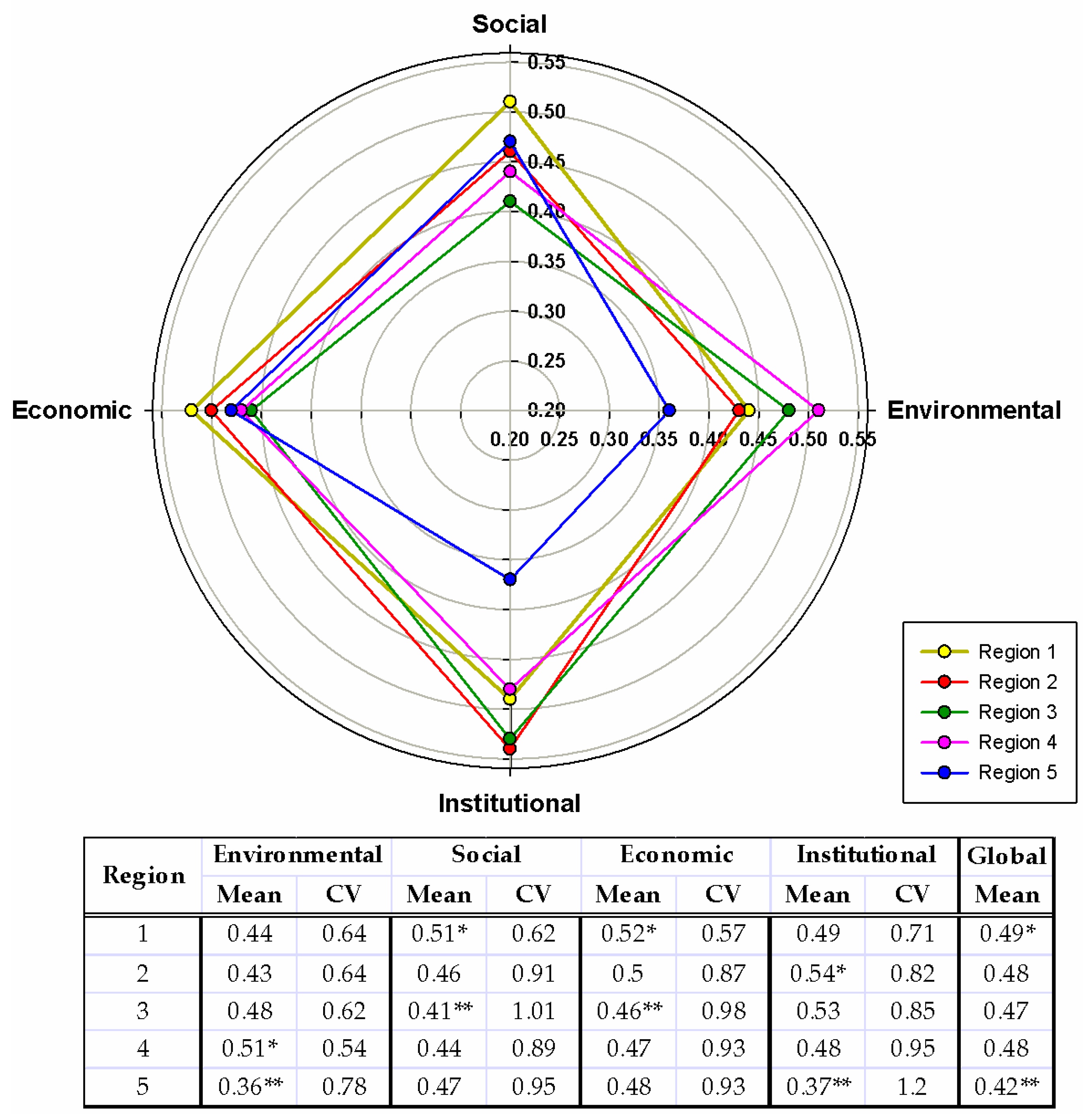
3.1. Identification of Similar Groups

The k-medoids analysis was performed from 14 input variables, including four PCs from the social subsystem, two PCs from the economic, five PCs from the environmental, and three variables from the institutional. The Silhouette consistency index determined the adequate number of similar regions to be five given the characteristics of the analyzed urban sub-basins (Figure 4).

The conditions of the regions are described by the averages of the normalized variables from each subsystem (Figure 5). These values created distinct regions. High values indicate that a region has better conditions for IWRM, and, correspondingly, more of its descriptive variables have values closer to one. In this sense, region 1 has, on average, the best conditions given the global mean of the four evaluated subsystems (0.49), and region 5 has the worst conditions (0.42). However, these averages do not reflect specific characteristics within each region. Therefore, more detailed descriptions were outlined considering only the real values of the most representative variables, as several of the considered variables had similar behavior (Figure 6, Figure 7, Figure 8 and Figure 9).

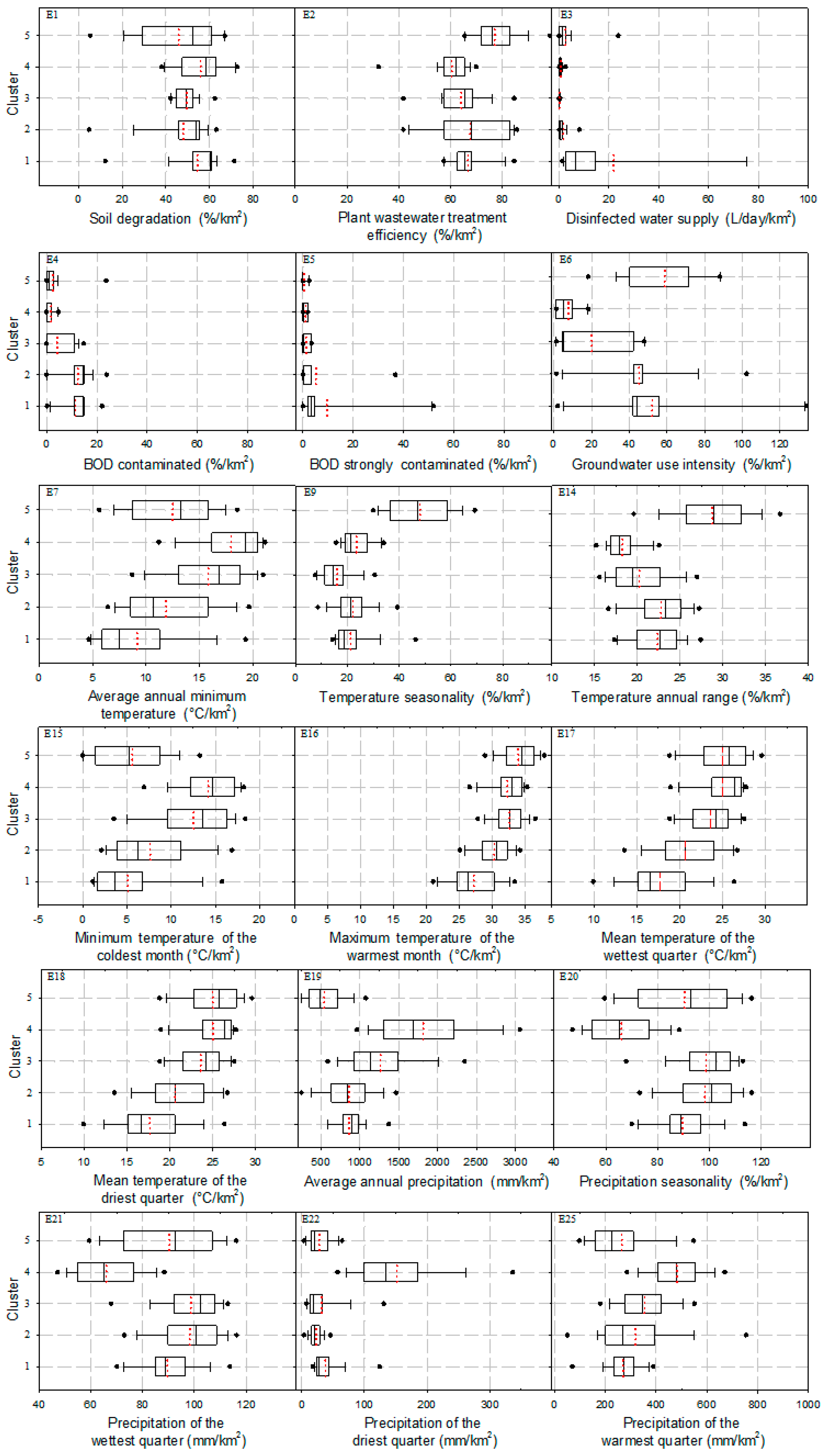
3.1.1. Environmental Subsystem

The Gulf of Mexico and the Yucatan Peninsula form part of region 4 that is characterized by having the best environmental conditions (0.51) (Figure 5). This region has the highest average annual minimum temperature (E7) in the country at 18 °C and an average annual maximum temperature (E8) of 29 °C. This is also the most humid region, with an average annual precipitation level (E19) of 1819 mm. However, there is large variability in the seasonality of precipitation (E20: 66%), as the rainy and dry seasons are not well-defined. Even in the driest quarter of the year, there is a considerable level of precipitation (E22: 152 mm). The excess of water in this region has allowed for the groundwater to be less intensively exploited (E6: 7.8%). However, vegetation loss in addition to the combined effect of high precipitation causes this region of the country to have the highest rate of soil degradation (E1: 56%).

In contrast, region 5 covers a large part of the northern region and is characterized by having the worst environmental conditions (0.36) for IWRM. Although the average annual minimum temperature is not the lowest (E7: 12.5 °C) and the average annual maximum temperature is not the highest (E8: 28 °C), the seasonality in temperature shows the largest variability (E9: 48%). The annual range in temperature (E14) reflects the existence of a 29 °C difference in temperature between the mean temperature of the coldest month (E11) and the maximum temperature of the hottest month (E12), making region 5 the most extreme in the country in terms of temperature. Poor temperature conditions may be exacerbated by low annual levels of precipitation (E19: 542 mm) and an overall water deficit since precipitation across all quarters and in both wet and dry seasons is the lowest in the country (E21: 325 mm, E22: 28 mm). The water deficit is evident in examining the additional precipitation variables, E23 to E26 (Figure 6), according to data reported by CONAGUA [33]. Furthermore, low levels of precipitation correspond with low rates of water erosion (E1: 46%). In this context and in other aspects, the resulting panorama positively affects factors that impact wastewater treatment and water quality since the efficiency of wastewater treatment plants (E2: 77%) and the percentage of BOD in water (E5: 0.4%) reflect the best conditions for these variables in comparison with other regions.

Region 3 has favorable environmental conditions (0.48). The climate is largely warm, with maximum temperatures of up to 36 °C and minimum temperatures as low as 3.6 °C. Seasonal variance in temperature (E9) is 16%, which indicates that this region does not have a large amplitude in temperature variability but rather has high temperatures throughout most of the year (Figure 6, parameters E15, E16, E17, and E18). Although this is not the most humid region, there is a high average annual precipitation (E19: 1266 mm/year), in addition to high levels of precipitation during the wettest quarter (E21: 721 mm/year) and the precipitation level of the wettest month (E23: 286 mm/month). The favorable climatic conditions are reflected in the region’s high water quality (E4 and E5), with values that do not surpass 4.5% BOD. Similarly, the intensity of groundwater use (E6) is low (20%), and the soil degradation by water erosion (E1) is moderate at 50% (Figure 6).

Regions 1 and 2 have nearly similar environmental conditions. Region 1 does not present favorable environmental conditions for IWRM (0.44) and is the coldest of the five regions (E7: 9.2 °C). In addition, the minimum temperature of the coldest month is the lowest (E15: 5.1 °C), and soil degradation (E1) and the intensity of groundwater use (E6) are also unfavorable (54.4% and 52.1%, respectively).

Meanwhile, the climate of region 2 can be categorized as temperate according to the National Institute of Ecology (INE, for its initials in Spanish) [57] and encompasses a large extension of the Trans-Mexican Volcanic Belt. This region covers nearly the entire Lerma-Chapala-Santiago river basin (LCS) with the exception of the metropolitan zones of Toluca, Queretaro, Guanajuato, and Jalisco. The LCS system may be classified as one of the most significant regions of the country in terms of its recent economic and demographic growth and the corresponding hydrological consequences that have occurred at the expense of the environment. Therefore, environmental services have been lost, and the vulnerability of basins has increased [57] resulting in a serious environmental liability for this region.

In region 2, the average annual minimum temperature (E7) is 11.9 °C, while the average annual maximum temperature (E8) is 26.8 °C. The annual range in temperature (E14) is 23 °C, measured from the minimum temperature of the coldest month (E15: 7.6 °C) to the maximum temperature of the hottest month (E16: 30.3 °C). Average annual precipitation (E19) is 862 mm, very similar to that of region 1. Precipitation of the driest month of the year (E24) is 5.4 mm, while that of the coldest quarter of the year (E26) is 47 mm, representing among the lowest values for the country (Figure 6). In region 2, the average wastewater treatment plant efficiency (E2) is high in comparison to other regions (67.5%). However, the treatment of wastewater is not reflected in water quality, as measured by the percentage of BOD (E4) since this region has the highest rate of contamination (12%). This is potentially the result of the indirect impact of metropolitan areas (outside of this region), which affect the natural resources of surrounding sub-basins.

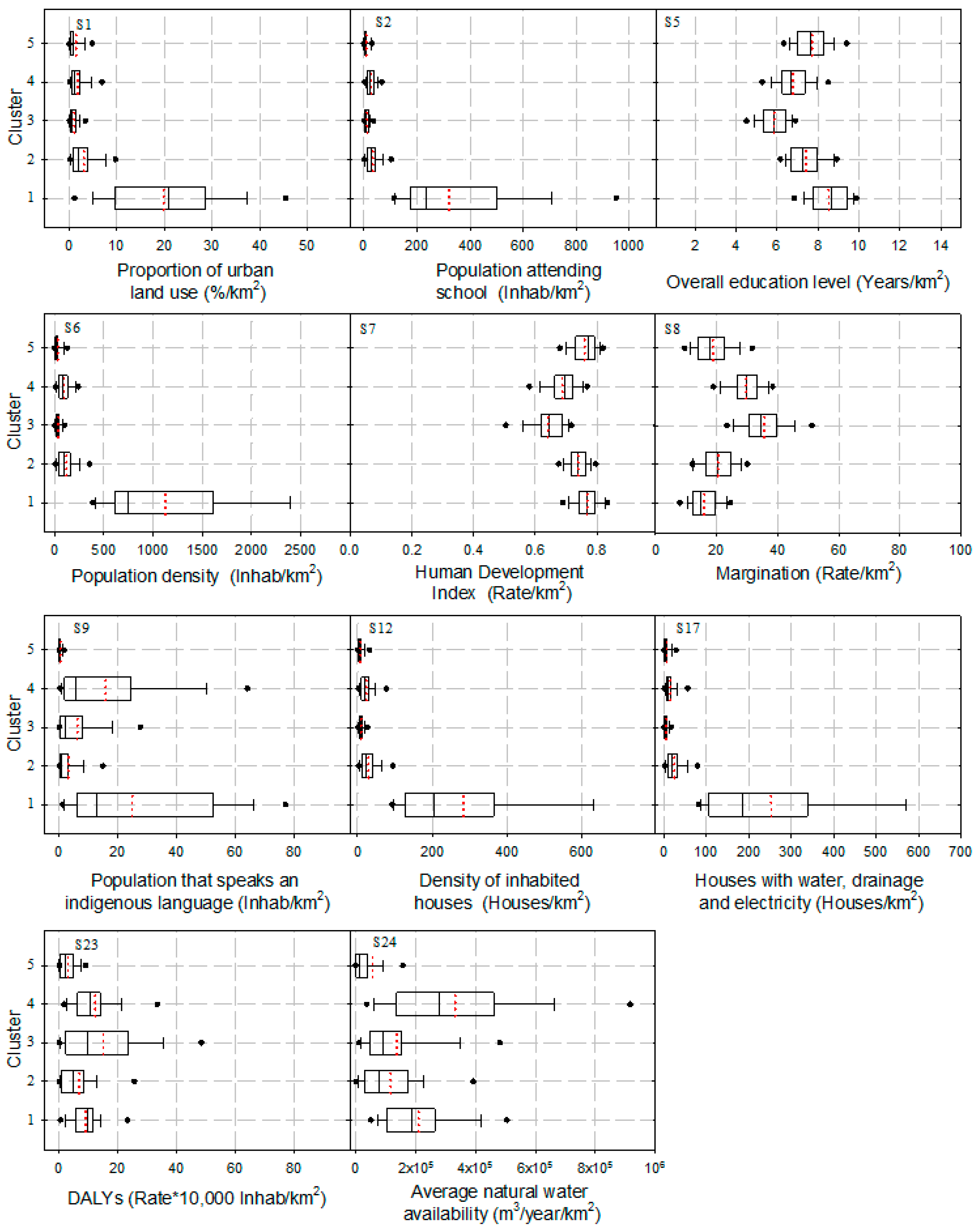
3.1.2. Social Subsystem

Within the classification, region 1 is the smallest and includes only 22 sub-basins that share mainly economic and social attributes. This region includes a large concentration of sub-basins that totally or partially encompass large urban areas (metropolitan areas), such as the Metropolitan Area of the Valley of Mexico (MAVM), Monterrey, Puebla, Guadalajara, and Toluca, among others. As a consequence, region 1 offers a promising panorama in terms of the provision of basic services and of a wide range of opportunities, as reflected by the average values of the social variables (0.51) (Figure 5).

This region also includes sub-basins with high population densities that speak indigenous languages (S9), such as the Miguel Ávila Camacho sub-basin (S6: 79 inhab/km²) in Puebla, and Río Otzolotepec sub-basin (S6: 69 inhab/km²) in the State of Mexico. However, it also encompasses sub-basins with low population densities (S6: 1 inhab/km²), for which the variability in this sense is significant (Figure 7). As with many urban centers, a large percentage of the population has a high education level (S5: 8.5 years) and attends school (S2: 322 inhab/km²). There are also high levels of access to basic services (water, electricity, wastewater infrastructure) (S17: 252 houses/km²) and a low level of marginalization (S8: 16/km²).

The average natural water availability (S24) ranges from 124 to 302 m³/inhab/year, which is on the low side of the spectrum in comparison to Monroy-Ortiz [29], who reported values from 168 to 5155 m³/inhab/year. The differences possibly reside in the fact that the region reported upon by the aforementioned author includes a larger number of basins, or all sub-basins that contain metropolitan areas.

A special case found in region 1 is that of the sub-basin that includes part of the MAVM (HAR XIII), which represents a large population center that places a huge pressure on water resources. Additionally, this region also generates the largest portion of the GDP (Ec4: 95,176 pesos/km²), has the highest concentration of population (S6: 1124 inhab/km²), and, in general, has a high standard of living in terms of the provision of basic services and housing (Figure 9). However, this has created a high demand for water, where, for example, the Lerma and Cutzamala regions must export around 30% of the water that is consumed in the MAVM [58]. This is a common problem in the large metropolitan areas of Mexico and a definitive and fundamental indicator of the state of water resources in urban sub-basins. The disadvantage is that national databases do not consider this indicator, and there are only several specific datasets at the national level that provide information on water deficits.

Regions 2 and 5 have similar averages for the social variables, overall (0.46 and 0.47, respectively). For region 2, the data demonstrates that social conditions are also favorable. After region 1, the percentage of urban areas (S1) within this region is the largest (3.2%). This is surely a consequence of the large economic and social expansion of the LCS system and its outlying growth contained in this area. Within the economic context, region 2 also has the best conditions after region 1 (Figure 5). Although population density (S6) is 128 inhab/km², only 28% of the population attends school (S2: 36 inhab/km²). The average education level (S5) is 7.4 years. Similarly, this region has the second highest values in terms of density of inhabited private houses (S12: 32 houses/km²) and houses with running water, drainage, and electricity (S17: 26 houses/km²) (Figure 7).

In comparison to region 2, region 5 has slightly superior social conditions (0.47), although this is also due to the fact that the population density (S6) is the lowest in the country (34 inhab/km²). Therefore, the density of inhabited private houses (S12: 8 houses/km²) and those with basic services (S17: 6.5 houses/km²) also have lower values in comparison with other regions. This is the least marginalized region of the country (S8: 19) with a Human Development Index (HDI) equal to region 1 (S7: 0.8), an average education level (S5) of 7.7 years, and 20% of the population attending school (S2). However, the social disadvantage of this region is associated with the low natural water availability, which is the lowest of the entire country (S24: 55,765 m³/ km²/year).

Region 3 covers the states of Michoacán, Guerrero, Oaxaca, and a large part of Chiapas, encompassing HARs IV, V, and XI (Figure 3). These states have the highest percentage of their population living in poverty [59]. Thus, region 3 is largely characterized by its deplorable social and economic situation. Urban land use (S1) barely arrives at 1.5% of the total area, and the education level is the lowest for all regions (S5: 6 years). Similarly, the HDI (S7) is low at 0.6/km², marginalization (S8) at 38/km², and the density of houses with basic services (S17) is 5.5 houses/km² (Figure 7). The high number of deaths due to intestinal disorders (S23: 15/10,000 inhab/km²) is likely related to the presence of waterborne diseases and the fact that medical services are located near or in larger cities despite the majority of the population living in rural areas. However, one positive characteristic for IWRM in this region is the high average natural availability of water (S24: between 334 and 52,649 m³/inhab/year).

Finally, 1.8% of region 4 is composed of urban land uses (S1), and the remaining portion is rural, containing a large portion of communities that speak indigenous languages (S9: 16 inhab/km²). This region also contains the highest average natural water availability in the country (S24: 331, 890 m³/km²/year). In social terms, rates of marginalization are high (S8: 29/km²), and the DALY due to intestinal disorders (S23) is also high at 12 per every 10,000 people. The average education level (S5) is 6.8 years, and the density of people attending school (S2) is 28/km² (Figure 7)

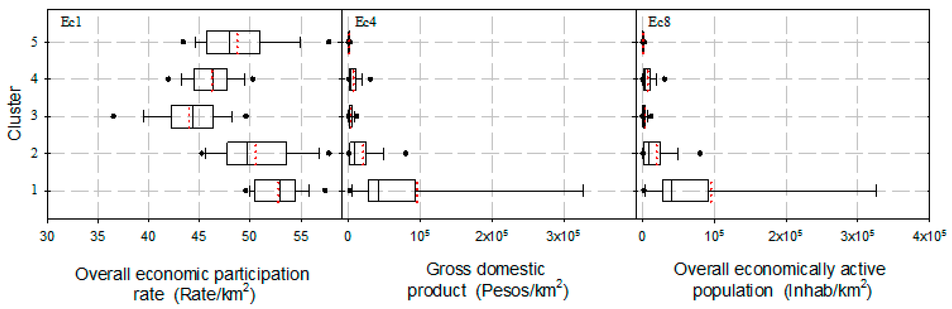
3.1.3. Economic Subsystem

As was expected, the best economic conditions were found in region 1 (0.52) (Figure 5). The GDP (Ec4) is the highest (95,175 pesos/km²), and this region also has the largest economically active population (Ec8: 472 inhab/km²) and the highest rate of economic participation (Ec1: 52.7%). In comparison, a large difference is observed with respect to region 5 that has low values for these indicators (Ec4: 614 pesos/km²; Ec8: 14 inhab/km²) (Figure 8). Undoubtedly, this aligns with the findings of Monroy-Ortíz [29], where it was found that 90% of the GDP is produced in the central region of the country, corresponding with the location of the largest metropolitan areas.

Interestingly, in region 3, the rate of economic participation (Ec1) is the lowest of the country (44%). The GDP (Ec4: 3032 pesos/km²) is not the lowest but is nonetheless considered low. Accordingly, the density of the economically active population is also very low (Ec8: 13 inhab/km²), reflecting the poverty of this region.

Meanwhile, as region 2 contains the largest number of urban centers following region 1, the economic conditions are also second to region 1 (Figure 5). The rate of economic participation (Ec1) is 51%, and the GDP (Ec4) is 20,252 pesos/km². The economically active population (Ec8) is 50 inhab/km² (Figure 8).

Region 5 has the highest GDP (Ec4: 612 pesos/km²), and the economically active population and the rate of economic participation are greater than in the poorest region of the country (Ec8: 14 inhab/km² and Ec1: 49%). However, in region 5 the provision of disinfected water (E3) and the average natural water availability (S24) represent several limits to an effective IWRM. Villanueva-Diaz et al. [60] mentions that the tendency in this region, the northern part of the country, is to extract water from aquifers at depths of up to 500 m, which is reflected in the high intensity of groundwater use (E6: 59%) and the construction of dams around superficial waterways to support the water demand from agricultural, public, urban, and industrial sectors. However, these actions are strategies that also require a large economic investment and put long-term water sustainability at risk.

Lastly, in region 4, the economic participation (Ec1) is 46%, and the GDP (Ec4) is 6931 pesos/km². The economically active population (Ec8) is 35 inhab/km². Thus, this region performs moderately well in terms of economic conditions in comparison to the other regions.

In agreement with Nieto [38], cities are the population centers where opportunities are concentrated, which translates to economic and social well-being. However, in the context of delimiting urban sub-basins, this data undoubtedly highlights the regional economic and social gaps in Mexico. This is an issue of concern for IWRM, and it is evident that these were decisive factors in separating the regions.

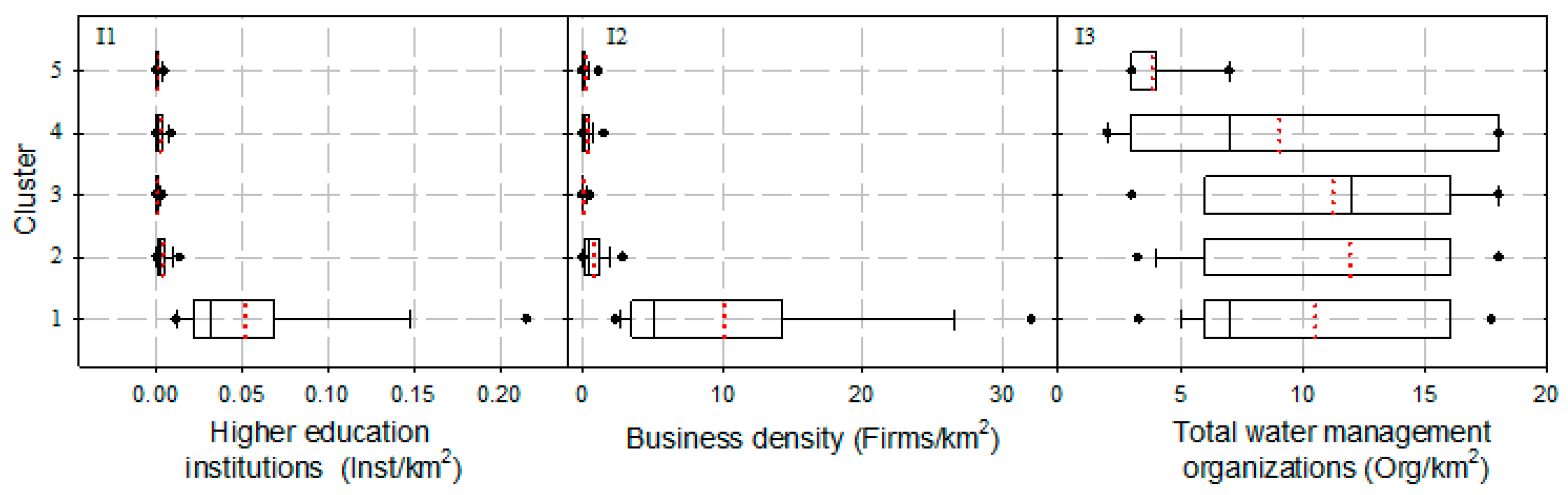
3.1.4. Institutional Subsystem

The density of superior education institutions (I1) and businesses (I2) per km² are the greatest in region 1 (I1: 0.1, I2: 10) (Figure 9). In the rest of the country, the density of superior education institutions (I1) is less than 0.1. This is due to the tendency toward centralization in the administration of resources, where economic resources are largely destined for the most urbanized areas [40]. In spite of this, region 1 does not have the most favorable institutional conditions (Figure 5).

The best conditions for the institutional subsystem were found in region 2 (0.54), although it has a lower density of superior education institutions (I1: 0.02 institutions/km²) than region 1. The density of businesses is also lower (I2: 1 business/km²), yet the number of water management organizations is higher (I3: 12 committee/km²) (Figure 9). Due to the large presence of these organizations (I3) and the lower density of businesses (I2), region 2 has the highest average for institutional well-being in the context of IWRM.

Meanwhile, region 3 has the lowest density of businesses (I2: 0.1 businesses/km²) but also has a high number of water management organizations (I3: 11 committee/km²). Region 4 has a moderate density of businesses (I2) at 0.4 per km², including nine water organizations per km². In this scenario, the region with the worst institutional conditions was region 5 (0.37), which has both a low density of businesses (I2: 0.2 businesses/km²) in addition to few water management organizations (I3: 4 committee/km²).

Although it is evident that the availability of digital and spatial information for the variables of this subsystem was insufficient, this is largely due to the lack of spatial data provided by water utilities departments. This study offers an initial approach with key variables in order to begin to characterize Mexico’s institutional subsystem.

4. Conclusions

This paper aims to contribute to several aspects of water policy convergence, which according to the characteristics mentioned by Bennet [9] as well as Dolowitz and Marsh [10], first involves the definition of planning goals and then the delineation of policies oriented toward improving specific conditions present in the sub-basins. While it is true that policies must be generic for the whole country, they should be nuanced in their application and based on the characteristics of each region and particular sub-basin. For this reason, the present paper proposes the delimitation of regions with similar environmental, social, and economic attributes in order to facilitate the elaboration of high-impact sustainable development strategies.

The current study has allowed for the identification of five regions based on the similarity of prevailing conditions in each one of the four subsystems considered in the systemic conceptual model, as relevant to the management of urban sub-basins and their corresponding basins in Mexico. The regionalization clusters and map here obtained demonstrate an overall panorama of the state of water resources in the urban sub-basins of the country. Since previous local studies have largely focused on environmental variables, such as precipitation, temperature [15], and hydrogeographic parameters [14], it is difficult to compare these results with those of the present due to the distinct parameters and goals of these investigations. However, due to the breadth of variables used in the current analysis, it was possible to adequately describe the five resulting regions (Figure 5, Figure 6, Figure 7 and Figure 8).

The economic and social subsystems have separated regions 1 and 2 as having the best conditions under these parameters, and these are the regions that also have the highest percentage of urbanization. To the contrary, region 3 has the worst conditions, as indicated by the economic and social variables, and it is subsequently the poorest region, coinciding with the states that are lagging behind in overall development indicators. Meanwhile, the environmental subsystem highlighted region 4 as having the best conditions and region 5 as having the worst, due to its extreme temperatures and low precipitation, as well as the large variability in both of these variables. Finally, the institutional subsystem underscores region 2 as having the best conditions, as it has the largest quantity of water management institutions. Region 5 was identified as the least favorable in this sense.

Likewise, this study integrated diverse subsystems that are influential in determining IWRM strategies for Mexico. It is notable that for the institutional subsystem, there was a lack of relevant information for the analysis (only three variables were found at a national level), which reflects the weaknesses and lack of transparency in interactions between institutions and civil society. Specifically, since IWRM implies an efficient and continual communication within institutions as well as among distinct institutions, the number of operating utilities or government dependencies does not necessarily accurately reflect the efficiency of water management in Mexico. Similarly, IWRM emphasizes public participation in the design of public policy, thereby establishing good governance through these interactions and promoting the creation of regulations and effective institutional procedures that would guide decision making and reinforce more egalitarian and sustainable processes. Yet these aspects were not sufficiently addressed in this study due to lack of information with the capacity to be spatially displayed at the national level. It would be interesting for future studies to integrate these additional aspects of an institutional analysis, including the number of local water committees or other nonprofits organizations related to water management. Although the latter are not official organisms (making their census difficult), they constitute an alternative means of water management in Mexico.

Finally, the environmental, social, economic, and cultural heterogeneity of Mexico requires a regional focus in order to propose improved solutions and strategies for water management, as current public policy does not efficiently address multidimensional problems but rather singularly focuses on specific problems and offers one-dimensional solutions [61]. Accordingly, uniform resolutions are extended across heterogeneous and unique regions. Such a standpoint leads to the creation of national paradigms that are impossible to implement locally, putting into place systematic behaviors that favor the lack of integrity in water management. Therefore, this justifies and explains the necessity to elaborate strategic IWRM plans with characteristics that are region-specific. Similarly, the notable differences between regions makes generalized plans inoperable for the entire country.

Future research should take into consideration the characterization of socio-ecological systems and their categorization into different regions, with the goal of identifying characteristics specific to each region that could guide strategic and regional management plans.

References

1. United Nations. United Nations Millennium Declaration; United Nations: New York, NY, USA, 2000. [Google Scholar]
2. Global Water Partnership (GWP). A Handbook for Integrated Water Resources Management in Basins; Elanders: Mölnlycke, Sweden, 2009. [Google Scholar]
3. Berkes, F.; Folke, C.; Colding, J. Linking Social and Ecological Systems: Management Practices and Social Mechanisms for Building Resilience; Cambridge University Press: Cambridge, UK, 2000. [Google Scholar]
4. Scott, C.A.; Banister, J.M. The dilemma of water management “regionalization” in Mexico under centralized resource allocation. Water Resour. Dev. 2008, 24, 61–74. [Google Scholar] [CrossRef]
5. Water, U. Status Report on the Application of Integrated Approaches to Water Resources Management; United Nations Environment Programme: Nairobi, Kenya, 2012. [Google Scholar]
6. Comisión Nacional del Agua (CONAGUA). Atlas Digital del Agua en México. Available online: http://www.CONAGUA.gob.mx/atlas/ (accessed on 25 April 2015).
7. Gobierno de la República. Ley de Aguas Nacionales; Diario Oficial de la Federación: México D.F., Mexico, 2013. [Google Scholar]
8. Perevochtchikova, M.; Arellano-Monterrosas, J.L. Gestión de cuencas hidrográficas: Experiencias y desafíos en México y Rusia. Rev. Latinoam. Recur. Nat. 2008, 4, 313–325. [Google Scholar]
9. Bennett, C.J. What is policy convergence and what causes it? Br. J. Political Sci. 1991, 21, 215–233. [Google Scholar] [CrossRef]
10. Dolowitz, D.; Marsh, D. Who learns what from whom: A review of the policy transfer literature. Political Stud. 1996, 44, 343–357. [Google Scholar] [CrossRef]
11. Ortega, R.R. Convergencia de política hacía la gestión integral de recursos hídricos en México. Rev. Mex. Análisis Político Adm. Pública 2015, 4, 67–88. [Google Scholar]
12. Salazar Adams, A.; Pineda Pablos, N. Factores que afectan la demanda de agua para uso doméstico en México. Reg. Soc. 2010, 22, 3–16. [Google Scholar]
13. Platt, R.H. Urban watershed management: Sustainability, one stream at a time. Environ. Sci. Policy Sustain. Dev. 2006, 48, 26–42. [Google Scholar] [CrossRef]
14. Allende, C.T.; Mendoza, M.E.; López Granados, E.M.; Morales Manilla, L.M. Hydrogeographical Regionalisation: An Approach for Evaluating the Effects of Land Cover Change in Watersheds. A Case Study in the Cuitzeo Lake Watershed, Central Mexico. Water Resour. Manag. 2009, 23, 2587–2603. [Google Scholar] [CrossRef]
15. Pineda-Martínez, L.F.; Carbajal, N.; Medina-Roldan, E. Regionalization and classification of bioclimatic zones in the central-northeastern region of México using principal component analysis (PCA). Atmósfera 2007, 20, 133–145. [Google Scholar]
16. Laaha, G.; Blöschl, G. A comparison of low flow regionalisation methods—Catchment grouping. J. Hydrol. 2006, 323, 193–214. [Google Scholar] [CrossRef]
17. Mertens, M.; Nestler, I.; Huwe, B. GIS-based regionalization of soil profiles with Classification and Regression Trees (CART). J. Plant Nutr. Soil Sci. 2002, 165, 39–43. [Google Scholar] [CrossRef]
18. Zhang, Q.; Wu, F.; Wang, L.; Yuan, L.; Zhao, L. Application of PCA integrated with CA and GIS in eco-economic regionalization of Chinese Loess Plateau. Ecol. Econ. 2011, 70, 1051–1056. [Google Scholar] [CrossRef]
19. Darand, M.; Daneshvar, M.M.R. Regionalization of Precipitation Regimes in Iran Using Principal Component Analysis and Hierarchical Clustering Analysis. Environ. Process. 2014, 1, 517–532. [Google Scholar] [CrossRef]
20. Shamshirband, S.; Gocić, M.; Petković, D.; Javidnia, H.; Ab Hamid, S.H.; Mansor, Z.; Qasem, S.N. Clustering project management for drought regions determination: A case study in Serbia. Agric. For. Meteorol. 2015, 200, 57–65. [Google Scholar] [CrossRef]
21. MacQueen, J. Some methods for classification and analysis of multivariate observations. In Proceedings of the 5-th Berkeley Symposium on Mathematical Statistics and Probability, Oakland, CA, USA, 21 June–18 July 1967; Volume 1, pp. 281–297.
22. Velmurugan, T.; Santhanam, T. Computational Complexity between K-Means and K-Medoids Clustering Algorithms for Normal and Uniform Distributions of Data Points. J. Comput. Sci. 2010, 3, 363–368. [Google Scholar] [CrossRef]
23. Di Giuseppe, E.; Jona Lasinio, G.; Esposito, S.; Pasqui, M. Functional clustering for Italian climate zones identification. Theor. Appl. Climatol. 2013, 114, 39–54. [Google Scholar] [CrossRef]
24. Park, H.-S.; Jun, C.-H. A simple and fast algorithm for K-medoids clustering. Expert Syst. Appl. 2009, 36, 3336–3341. [Google Scholar] [CrossRef]
25. Kaufman, L.; Rousseeuw, P.J. Partitioning around medoids (program pam). In Finding Groups in Data: An Introduction to Cluster Analysis; John Wiley & Sons, Inc.: Hoboken, NJ, USA, 1990; pp. 68–125. [Google Scholar]
26. Ng, R.T.; Han, J. CLARANS: A method for clustering objects for spatial data mining. IEEE Trans. Knowl. Data Eng. 2002, 14, 1003–1016. [Google Scholar] [CrossRef]
27. Baarsch, J.; Celebi, M.E. Investigation of internal validity measures for K-means clustering. In Proceedings of the International MultiConference of Engineers and Computer Scientists, Hong Kong, China, 12–16 March 2012; Volume 1, pp. 14–16.
28. Ahmed, R.; Mahmood, K.; Kausar, A. Socio-Agricultural Correlation and Regionalization: A Case of the Districts of Pakistan. J. Basic Appl. Sci. 2014, 10, 7–19. [Google Scholar] [CrossRef]
29. Monroy-Ortiz, R. Los sistemas urbanos de cuenca en México: Transitando a estrategias integrales de gestión hídrica. Econ. Soc. Territ. 2013, 13, 151–179. [Google Scholar] [CrossRef]
30. Carabias, J.; Landa, R. Agua, Medio Ambiente y Sociedad. Hacia la Gestión Integral de los Recursos Hídricos en México; UNAM: México D.F., Mexico, 2005. [Google Scholar]
31. García, E. Clasificación de Köppen, Modificado por García, E.; CONABIO: México D.F., Mexico, 1998. [Google Scholar]
32. Ceballos, G.; Valenzuela, D.; Ceballos, G.; Martínez, L.; García, A.; Espinoza, E.; Bezaury, J.J.; Dirzo, R. Diversidad, Amenazas y Áreas Prioritarias para la Conservación de las Selvas Secas del Pacífico de México; Fondo de Cultura Económica, CONABIO and CONANP: México D.F., Mexico, 2010. [Google Scholar]
33. Comisión Nacional del Agua (CONAGUA). Atlas del Agua en México 2012; Secretaría de Medio Ambiente y Recursos Naturales: México D.F., Mexico, 2012. [Google Scholar]
34. Gobierno de la República. Programa Nacional Hídrico 2014–2018; Diario Oficial de la Federación: México D.F., Mexico, 2014. [Google Scholar]
35. Fondo para la Comunicación y la Educación Ambiental (FCEA), Centro Mexicano de Derecho Ambiental (CEMDA), Presencia Mexicana Ciudadana Mexicana (P.M.C.M.). Agua en México: Lo que Todos y Todas Debemos Saber; Fondo Educación Ambiental: México D.F., Mexico, 2006. [Google Scholar]
36. Instituto Nacional de Estadística y Geografía (INEGI). Referencias Geográficas y Extensión Territorial de México; INEGI: México D.F., Mexico, 2010. [Google Scholar]
37. Instituto Nacional de Estadística y Geografía (INEGI). Censo de Población y Vivienda. 2010. Available online: http://www.inegi.org.mx/est/contenidos/proyectos/ccpv/cpv2010/Default.aspx (accessed on 13 August 2015).
38. Nieto, A.T. Las economías de las zonas metropolitanas de México en los albores del siglo XXI. Estud. Demogr. Urbanos 2013, 28, 545–591. [Google Scholar]
39. Hearne, R.R. Evolving water management institutions in Mexico. Water Resour. Res. 2004, 40, W12S04. [Google Scholar] [CrossRef]
40. Parnreiter, C. Ciudad de México: El camino hacia una ciudad global. EURE Santiago 2002, 28, 89–119. [Google Scholar] [CrossRef]
41. Instituto Nacional de Estadística y Geografía (INEGI). Economía, Cuadro Resumen. Available online: http://www3.inegi.org.mx/sistemas/temas/default.aspx?s =est&c=23824 (accessed on 15 October 2015).
42. Gobierno de la República. Plan Nacional de Desarrollo 2013–2018; Diario Oficial de la Federación: México D.F., Mexico, 2013. [Google Scholar]
43. Comisión Nacional del Agua (CONAGUA). Estadísticas del Agua en México; Secretaría de Medio Ambiente y Recursos Naturales: México D.F., Mexico, 2015. [Google Scholar]
44. Comisión Nacional del Agua (CONAGUA). Estadísticas del Agua en México; Secretaría de Medio Ambiente y Recursos Naturales: México D.F., Mexico, 2013. [Google Scholar]
45. Hijmans, R.J.; Cameron, S.E.; Parra, J.L.; Jones, P.G.; Jarvis, A. Very high resolution interpolated climate surfaces for global land areas. Int. J. Climatol. 2005, 25, 1965–1978. [Google Scholar] [CrossRef]
46. Eastman, J.R. IDRISI Selva; Clark University: Worcester, MA, USA, 2012. [Google Scholar]
47. Environmental Systems Research Institute (ESRI). ArcGIS Desktop: Release 10; ESRI: Redlands, CA, USA, 2011. [Google Scholar]
48. Eastman, J.R. Guide to GIS and Image Processing; Clark University: Worcester, MA, USA, 2012. [Google Scholar]
49. Landeta, J. Current validity of the Delphi method in social sciences. Technol. Forecast. Soc. Chang. 2006, 73, 467–482. [Google Scholar] [CrossRef]
50. Tan, L.; Liu, H.; Ma, Y.; Wu, L.; Min, Q.; Gao, S.; Liu, J. Quantification of spatial difference of sustainability in the Taihang Mountain area of Hebei Province, China, with its information platform and GIS. J. Food Agric. Environ. 2011, 9, 740–747. [Google Scholar]
51. Statgraphics Centurion V15.2; Statpoint Technologies: Warrenton, VA, USA, 2009.
52. Kaiser, H.F. The application of electronic computers to factor analysis. Educ. Psychol. Meas. 1960, 20, 141–151. [Google Scholar] [CrossRef]
53. Shlens, J. A Tutorial on Principal Component Analysis: Derivation, Discussion and Singular Value Decomposition. 2003. Available online: https://www.cs.princeton.edu/picasso/mats/PCA-Tutorial-Intuition_jp.pdf (accessed on 28 December 2016).
54. Rousseeuw, P.J. Silhouettes: A graphical aid to the interpretation and validation of cluster analysis. J. Comput. Appl. Math. 1987, 20, 53–65. [Google Scholar] [CrossRef]
55. Lletí, R.; Ortiz, M.C.; Sarabia, L.A.; Sánchez, M.S. Selecting variables for k-means cluster analysis by using a genetic algorithm that optimises the silhouettes. Anal. Chim. Acta 2004, 515, 87–100. [Google Scholar] [CrossRef]
56. R Development Core Team. R: A Language and Environment for Statistical Computing; R Foundation for Statistical Computing: Vienna, Austria, 2009; Available online: https://www.r-project.org (accessed on 15 October 2015).
57. Instituto Nacional de Estadística (INE). Atlas de la Cuenca Lerma-Chapala: Construyendo una Visión Conjunta; Cotler Avalos, H., Mazari Hiriart, M., de Anda Sánchez, J., Eds.; INE: México D.F., Mexico, 2006. [Google Scholar]
58. Legorreta, J. El Agua y la Ciudad de México de Tenochtitlán a la Megalópolis del Siglo XXI; Universidad Autónoma Metropolitana: México D.F., Mexico, 2006. [Google Scholar]
59. Consejo Nacional de Evaluación de la Política de Desarrollo Social (CONEVAL). Evolución de la Pobreza en México. Medición de la Pobreza. 2014. Available online: http://www.coneval.gob.mx/Medicion/MP/Paginas/Pobreza_2014.aspx (accessed on 14 October 2015).
60. Villanueva-Diaz, J.; Stahle, D.W.; Luckman, B.H.; Cerano-Paredes, J.; Therrell, M.D.; Cleaveland, M.K.; Cornejo-Oviedo, E. Winter-spring precipitation reconstructions from tree rings for northeast Mexico. Clim. Chang. 2007, 83, 117–131. [Google Scholar] [CrossRef]
61. Huang, B.; Fan, T.; Li, Y.; Wang, Y. Division scheme for environmental management regionalization in China. Environ. Manag. 2013, 52, 289–307. [Google Scholar] [CrossRef] [PubMed]
62. Instituto Nacional para el Federalismo y el Desarrollo Municipal. Sistema Nacional de Información Municipal (SNIM). Available online: http://www.snim.rami.gob.mx/ (accessed on 14 October 2015).
63. Gómez-Albores, M.A. Modelación Geomática de Medidas de Frecuencia y de Asociación, Aplicada a Enfermedades Vinculadas con el Agua. Ph.D. Thesis, Universidad Autónoma del Estado de México, Facultad de Ingeniería, Centro Interamericano de Recursos del Agua (CIRA), Toluca de Lerdo, Mexico, 2012. [Google Scholar]
64. Secretaría de Economía. Sistema de Información Empresarial Mexicano. Available online: http://www.siem.gob.mx/siem/portal/consultas/ligas.asp?Tem=1 (accessed on 14 October 2015).
65. Asociación Nacional de Universidades e Instituciones de Educación Superior en México (ANUIES). Información Estadística de Educación Superior. Available online: http://www.anuies.mx/informacion-y-servicios/informacion-estadistica-de-educacion-superior (accessed on 14 October 2015).
66. Secretaría del Medio Ambiente y Recursos Naturales (SEMARNAT). Sistema Nacional de Indicadores Ambientales. Available online: http://apps1.semarnat.gob.mx/dgeia/indicadores14/conjuntob/00_conjunto/temas.html?De=SNIA (accessed on 14 October 2015).
Figure 1. Political and hydrological limits of Mexico. * Hydrological Administrative Region (HAR).
Water 09 00014 g001
Figure 2. Regionalization methodology for delimiting urban sub-basins based on socio-ecological variables (See Appendix B for description of variables). HAR: Hydrological Administrative Region, PCA: Principal Component Analysis, PAM: Partitioning Around Medoids.
Water 09 00014 g002
Figure 3. Principal component weights. Subsystem: (a) social; (b) environmental; (c) economic. Ev: explained variance.
Water 09 00014 g003
Figure 4. Regionalization of the urban sub-basins. * Hydrological-Administrative Region (Roman numerals). The upper right graph show Silhouette index values from 2 to 20 division groups, dashed red line is the best cluster division for data.
Water 09 00014 g004
Figure 5. Average and variation coefficient of normalized values by subsystem and region. CV: Coefficient of variation. * Best region, ** Worst region.
Water 09 00014 g005
Figure 6. Regional environmental characteristics with real values. Average value is the dotted red line.
Water 09 00014 g006
Figure 7. Regional social characteristics with real values. Average value is the dotted red line.
Water 09 00014 g007
Figure 8. Regional economic characteristics with real values. Average value is the dotted red line.
Water 09 00014 g008
Figure 9. Regional institutional characteristics with real values. Average value is the dotted red line.
Water 09 00014 g009