Article

Comparing Sprinkler and Surface Irrigation for Wheat Using Multi-Criteria Analysis: Water Saving vs. Economic Returns

Linking Landscape, Environment, Agriculture and Food (LEAF), Instituto Superior de Agronomia, University of Lisbon, Tapada da Ajuda, 1349-017 Lisboa, Portugal
*
Author to whom correspondence should be addressed.
Water 2017, 9(1), 50; https://doi.org/10.3390/w9010050
Submission received: 28 October 2016 / Revised: 5 January 2017 / Accepted: 9 January 2017 / Published: 13 January 2017

Abstract

:
Coping with water scarcity using supplemental irrigation of wheat (Triticum aestivum L.) in the semi-arid northeast Syria is a great challenge for sustainable water use in agriculture. Graded borders and set sprinkler systems were compared using multi-criteria analysis. Alternative solutions for surface irrigation and for sprinkler systems were developed with the SADREG and the PROASPER design models, respectively. For each alternative, two deficit irrigation strategies were considered, which were characterized using indicators relative to irrigation water use, yields and water productivity, including farm economic returns. Alternatives were ranked considering two contrasting priorities: economic returns and water saving. A first step in ranking led to a selection of graded borders with and without precise land levelling and of solid set and semi-permanent sprinkler systems. Precise-levelled borders were better for water saving, while non-precise ones ranked higher for economic returns. Semi-permanent set systems have been shown to be better in economic terms and similar to solid set systems when water saving is prioritized. Semi-permanent sprinkler systems rank first when comparing all type of systems together regardless of the considered deficit irrigation strategy. Likely, border irrigation is appropriate when wheat is in rotation with cotton if the latter is surface irrigated. When peace becomes effective, appropriate economic incentives and training for farmers are required to implement innovative approaches.

1. Introduction

The main cultivated crops in northeast Syria are wheat and cotton. Wheat (Triticum durum and T. aestivum L.) was originated in the Fertile Crescent region, which comprises northeast Syria, around 10,000 years B.C. [1]. The largest wheat cultivated area, representing 39% of the total country production (45% irrigated and 55% rainfed), was the Al-Hassakeh Governorate, in the Al-Khabour basin, northeastern Syria [2]. However, water scarcity has gradually increased in the last few years due to excessive overdraft of the groundwater in both Syria and Turkey [3,4,5,6,7], as well as due to climate change [8]. To face the related problems, a national irrigation modernization project has been implemented [9,10,11]. Although all efforts were destroyed by the on-going war, preparing for peace is paramount.
The need for supplemental irrigation of winter wheat in Syria has been well identified in several studies, including advocating the adoption of deficit irrigation to cope with water scarcity [12,13,14,15,16,17]. Other studies conducted in the Near East and North Africa region confirm results obtained in Syria, e.g., [18,19]; including the search for quality and to cope with drought stress [20]. The need for supplemental irrigation of wheat was also reported when considering adaptation to climate change [21].
The traditional surface irrigation systems generally have low irrigation performance due to several problems, including non-levelled land and poor irrigation management. However, surface irrigation performance could be improved when adopting well-designed and managed systems and appropriate irrigation scheduling [22,23]. Using multi-criteria analysis (MCA) for selecting and ranking alternative surface and drip irrigation systems for cotton, it could be concluded that improved furrow irrigation may lead to higher farm economic returns than drip irrigation, but low cost drip systems may be feasible and lead to appreciable water saving [24]. A similar MCA study aimed at comparing set sprinkler and modernized border irrigation for winter wheat could be considered, i.e., for assessing the feasibility of changes in irrigation technologies as a means to better valuing water in wheat production. Yigezu et al. [10] reported that improving the irrigation schedule jointly with adopting sprinkler technologies may lead to water saving with increased water productivity and farmer profits. However, as analyzed by Lecina et al. [25], replacing surface irrigation by sprinkling may not lead to water savings because improved irrigation and cultivation conditions may lead to an increased demand for production factors, including water.
Multi-criteria analysis was selected because it combines various criteria, often contradictory, of an economic, environmental and technical nature, as well as relative to water saving. Furthermore, it admits various schemes for prioritizing and ranking the technical solutions being compared [26,27,28]. MCA adapts well to selecting fertilizing and irrigation options [29,30], to supporting improvements in irrigation management and water saving [28,31,32] or to comparing and selecting irrigation methods [24,33]. As an alternative to MCA, various methods are available to select irrigation systems through considering costs, production parameters, yields and water use [34,35,36,37]. However, the interdependency among factors and criteria is better considered using MCA, as for the examples above, or with the analytical hierarchy process used by Montazar and Behbahani [38] for irrigation system selection.
This study, based on field data of supplemental irrigated winter wheat in the Ras-El-Ain area (northeast Syria), aims at comparing set sprinkler and borders irrigation using MCA taking into account the performance of both methods in terms of water saving and economic returns when considering mild and moderate-deficit irrigation. The adoption of MCA is justified because there is the need to make compatible two central, but contradictory issues: water saving and farm economic returns.

2. Materials and Methods

2.1. Experimental Site

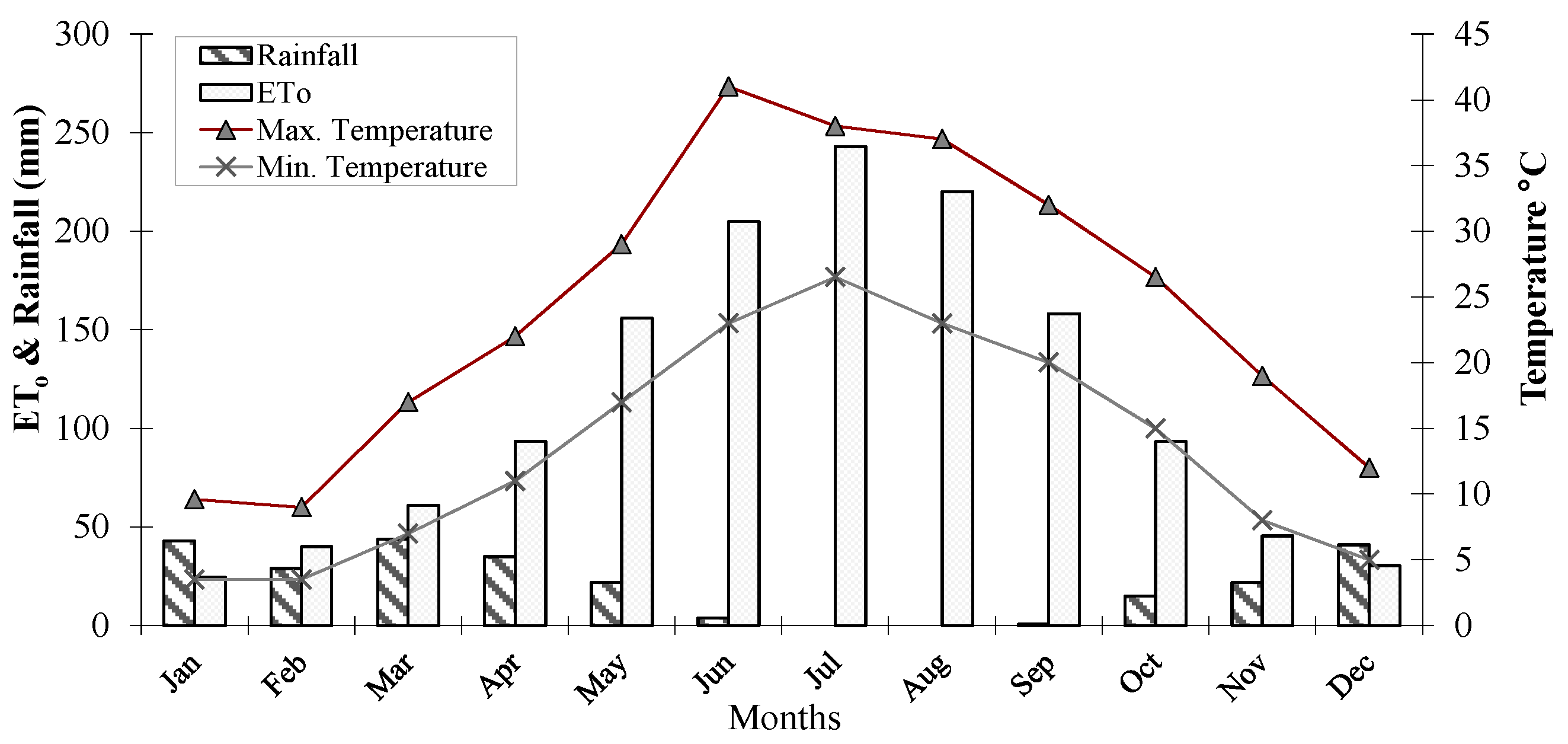
The study area was located at Ras-El-Ain (latitude 36°50’ N, longitude 40°4’ E) in the Al-Khabour basin, Al-Hassakeh region, northeast Syria. The area has a semi-arid climate, as shown in Figure 1, with low rainfall. Reference evapotranspiration (ETo), computed for a 10-year period (1993–2002) with the FAO-Penman Monteith method [39], exceeds precipitation for most of the months. The topography is slightly undulated with land elevations ranging from 165 to 325 m.
Soils are predominantly clay loams, with an average textural composition of 30% sand, 31% silt and 39% clay. Soil water content at 30 kPa (field capacity) is 0.37 cm3·cm−3 and at 1550 kPa (permanent wilting point) is 0.23 cm3·cm−3, resulting in a total available water of 140 mm. The soil infiltration characteristics were analyzed in a previous study [23], and the resulting Kostiakov infiltration curve is:
Z = 0.0118 τ 0.3227 + 0.000167 τ
where Z is the cumulative infiltration per unit width of the borders (m3·m−1) and τ is the infiltration opportunity time (min). The observed soil basic infiltration rate is 4.1 mm·h−1 [23].
The wheat crop is commonly sown by December or early January and is harvested by mid-June. Supplemental irrigation is often applied, generally using traditional graded borders. The actual surface irrigation performances and respective potential improvements have been recently analyzed [23]. For the present study, a wheat season of 165 days was considered, the sowing date being 1 January. The average observed yield varied from 5000 to 5250 kg·ha−1.
The field experiments were performed in a sprinkling field and in borders of 50, 100 and 200 m in length, a longitudinal slope of 0.8% and a null cross slope, which were divided into various widths depending on the available flow rate. Two independent wells with a discharge of 30 and 40 L·s−1 provided water for the supplemental irrigation. A topographic survey and a land smoothing operation were performed to provide for a uniform slope.

2.2. Modelling

Various sets of alternatives for both border and set sprinkler systems were developed using respectively the models SADREG [40] and PROASPER [41]. Each alternative was then characterized by appropriate performance indicators relative to water saving and economic results.
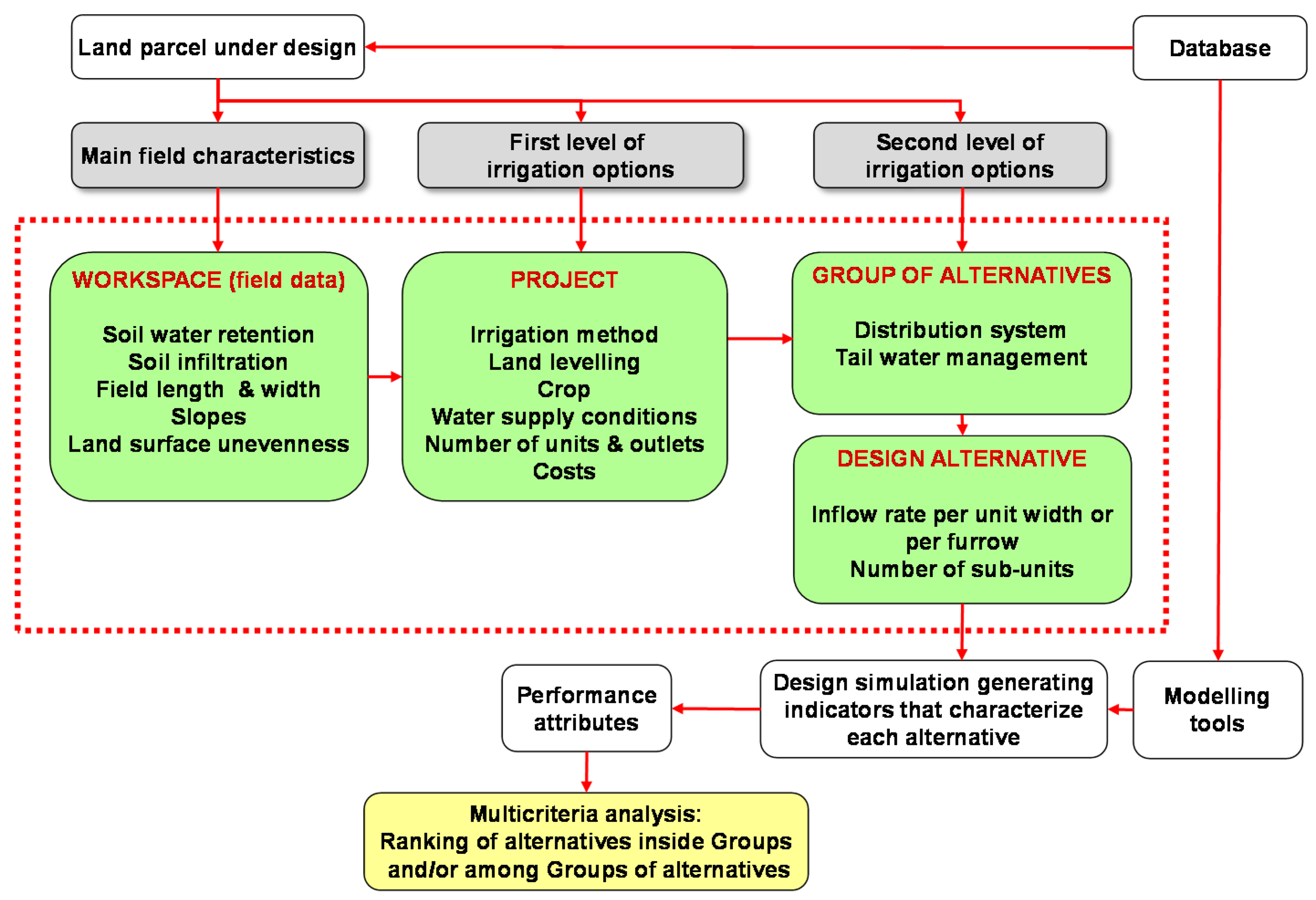
SADREG is a farm surface irrigation design model whose hydraulic simulations are performed interacting with the simulation model SIRMOD [42]. The procedure for creating the required design alternatives follow various steps, as depicted in Figure 2. The workspace deals with main field characteristics, including topography, and is common to all alternatives. The “project” groups all items required to design the alternatives, e.g., land levelling. The next level consists of grouping the alternatives in terms of water distribution to the borders and tail water management. Finally, the alternatives are designed, taking into consideration the inflow rates and related border width.
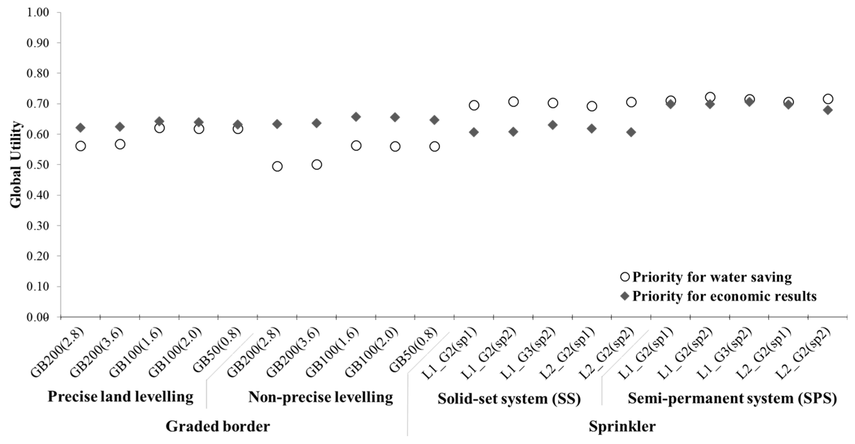
Considering results previously obtained [
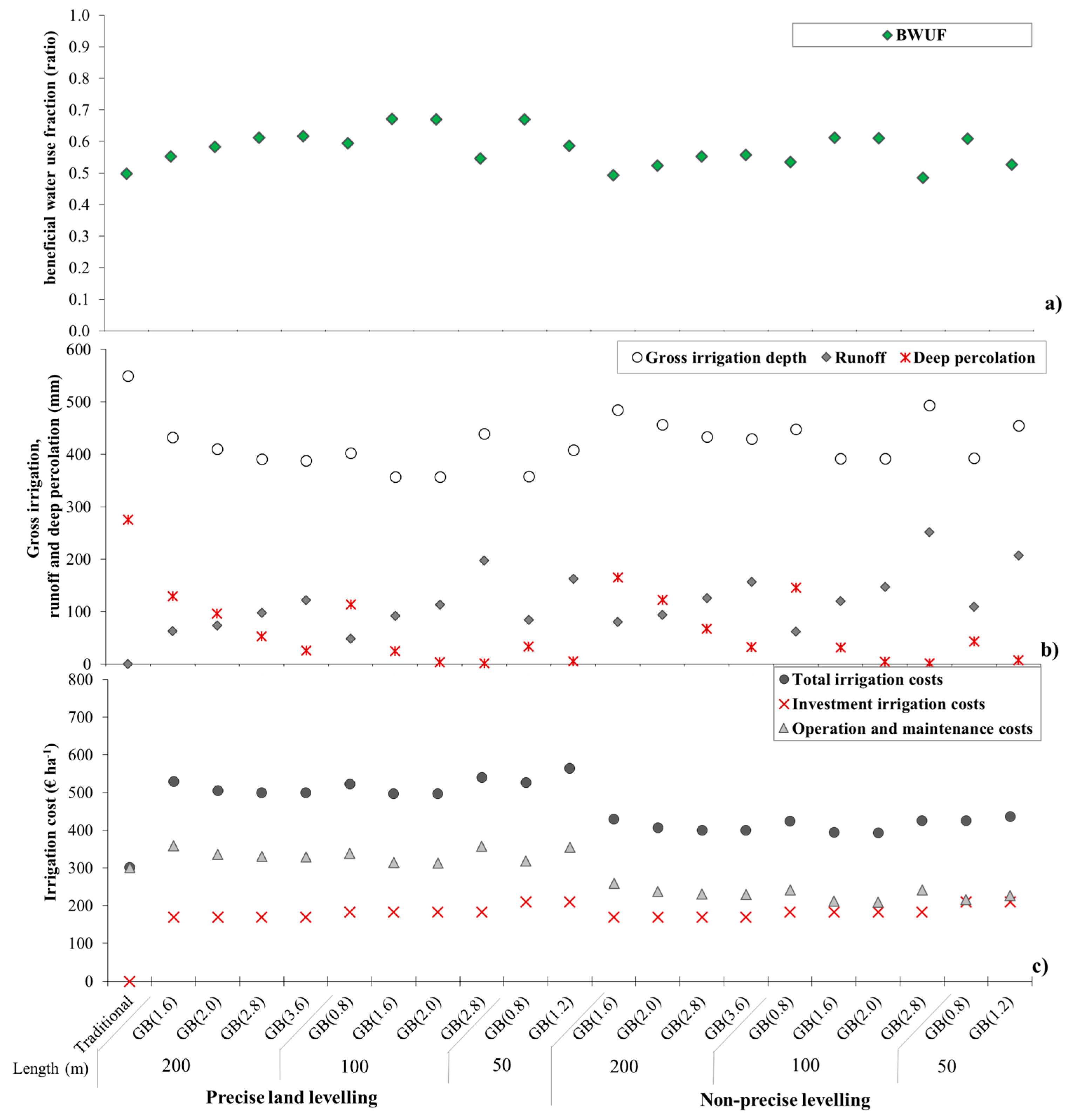
23], this application focused on graded border irrigation with and without precision land levelling, respectively GBPL and GBNPL. Contrary to GBPL, GBNPL has reduced investment, but does not allow achieving high distribution uniformity and good irrigation performances. Design options included flat soil surface, lay-flat gated tubing for in-field water distribution and open-tail end with reuse in lower downstream fields. The alternatives resulted from the combination of different field lengths (50 m, 100 m and 200 m) with various inflow rates per unit width (0.8, 1.2, 1.6, 2.0, 2.8 and 3.6 L·s−1·m−1). Hydraulic computations were performed using a Manning’s roughness coefficient of 0.16 s·m−1/3 as described by Darouich et al. [23].
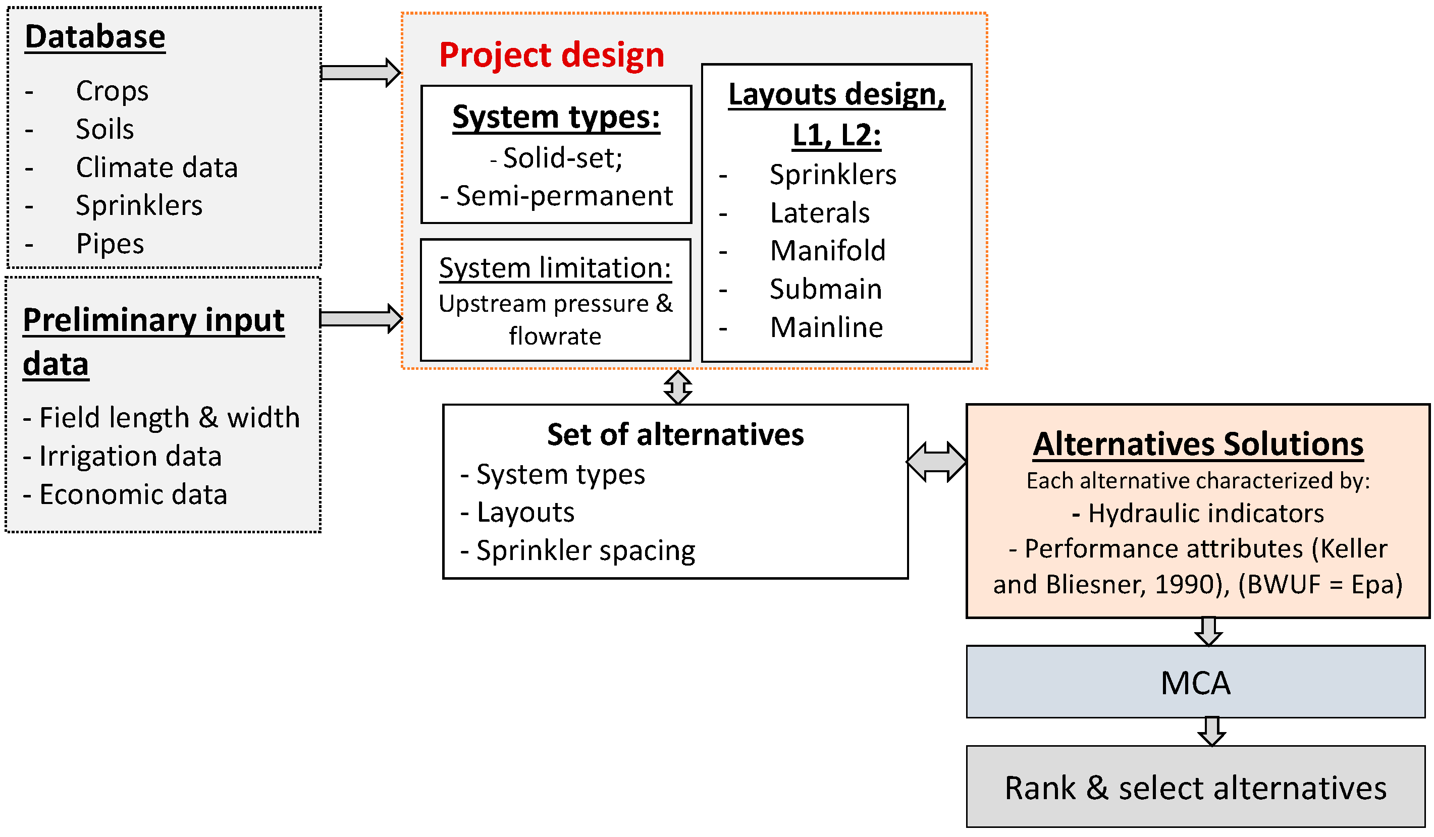
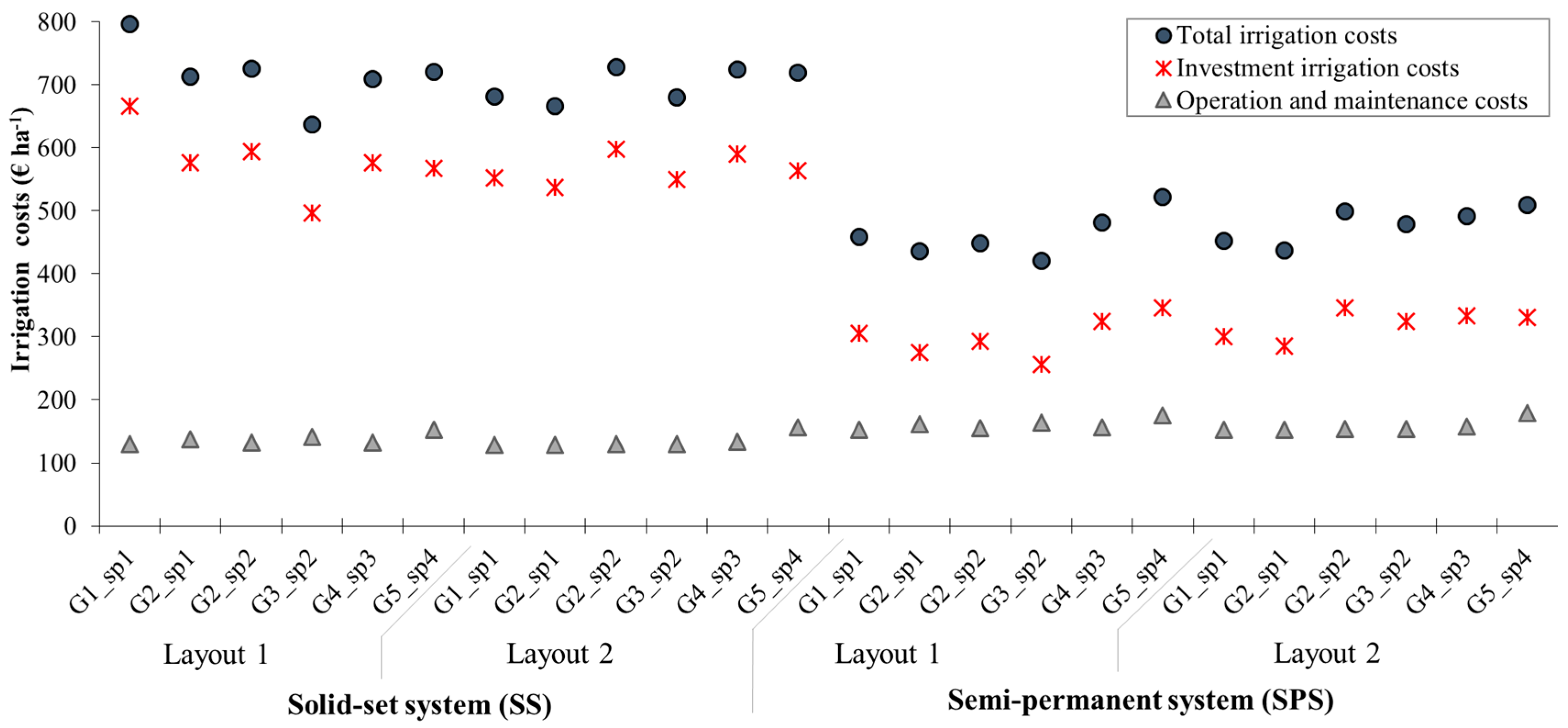
PROASPER is a design model for set sprinkler systems as represented in the flowchart of Figure 3. In the present work, solid set (SS) and semi-permanent gridded pipe systems (SPS) were considered. The design is performed through an iterative procedure, with automatic search in the database of the pipes and sprinklers whose characteristics meet the user’s choices in terms of pipe length, sprinkler spacing, application rates and hydraulic performance. The methodology for pipe sizing follows that proposed by Keller and Bliesner [43]. The pressure head variation among sprinklers operating simultaneously can be decided by the user, but should not exceed 20% of the design pressure, thus resulting in a sprinkler discharge variation smaller than 10%. The flow velocity in pipes was limited to 1.5 m·s−1. The application rate was limited to the soil infiltration rate (4.1 mm·h−1).
The design application efficiency Epa (%) referring to a selected percentage (pa) of the area adequately irrigated, herein considered pa = 75%, was computed as proposed by Keller and Bliesner [43]:
E pa = DE pa   R e   O e
where DEpa is the distribution efficiency for pa (%), Re is the effective portion of applied water (decimal) and Oe is the ratio of water effectively discharged through sprinkler nozzles to total system discharge (decimal), which was assumed equal to 0.99 for a new and well-maintained system. Results of the simulation were compared with field evaluation results.
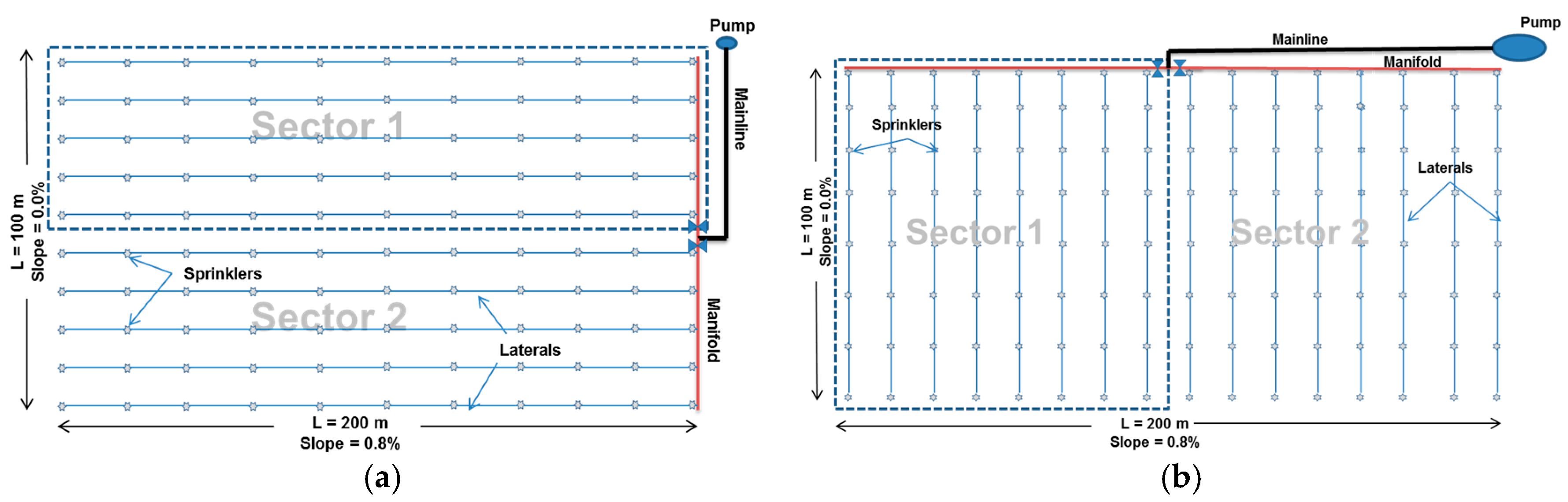
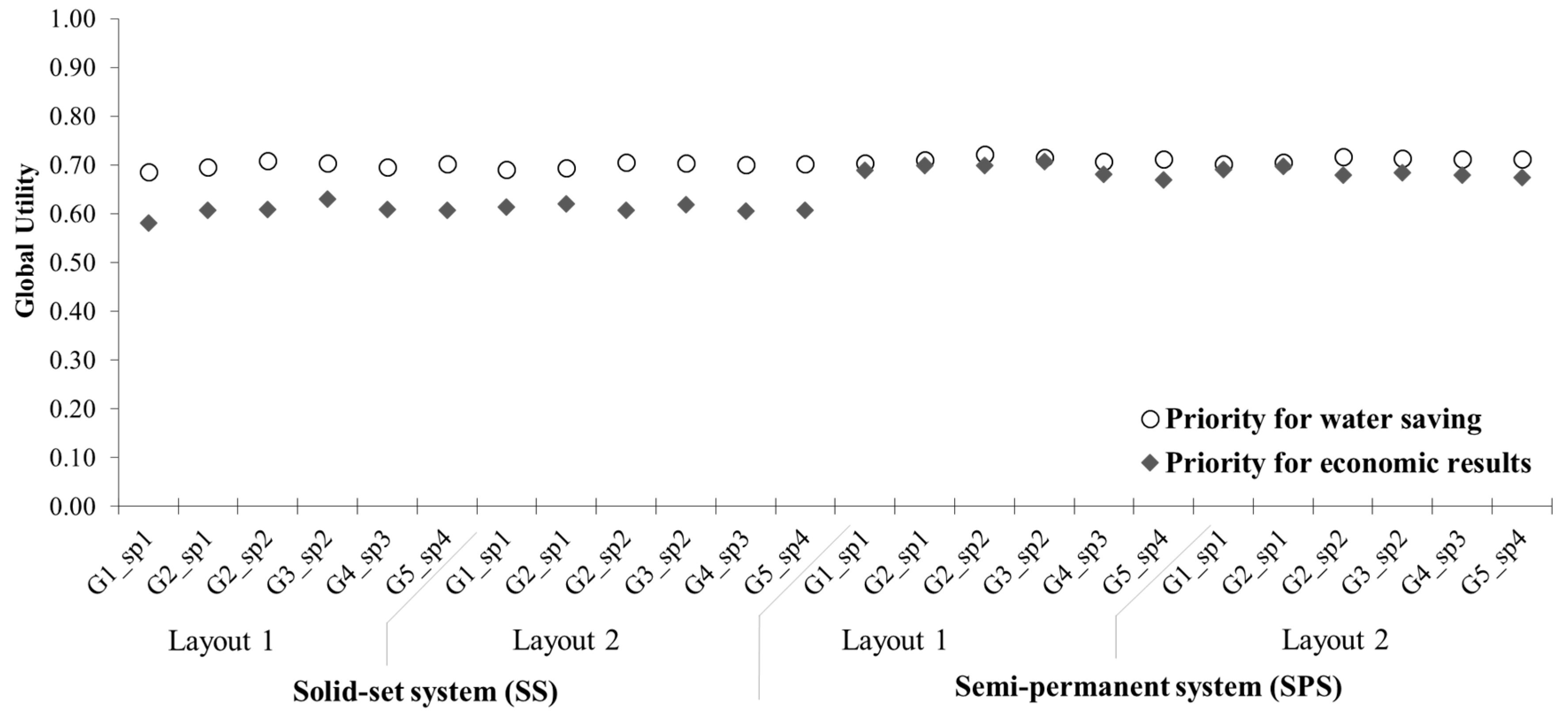
Sprinkler system alternatives were obtained by combining two pipe layouts (Figure 4), four types of sprinklers and five different spacings. The two layouts used, L1 and L2 (Figure 4), consisted of different positions of the laterals in relation to the manifolds, in both cases, dividing the field into two sectors. The sprinkler types (sp1, ..., sp4) and their characteristics, as well as the spacing tested (G1, …, G5) are reported in Table 1. The pipes adopted for the laterals and manifolds were of high-density polyethylene and for the main lines were PVC pipes. Pipe sizes were computed by the model when a target CU of 80% was given as the input. Model results include the mainline, submain, manifold and lateral pipe sizes, the pressure head and discharge of each sprinkler and their variation across the system.
The wheat irrigation schedules used as inputs in SADREG and PROASPER were obtained with the ISAREG model [44,45] previously validated for the region [13]. Two irrigation strategies were considered: (1) mild-deficit supplemental irrigation (MD), aiming at fulfilling the crop water requirements and ceasing irrigation 30 days before harvesting; and (2) moderate-deficit irrigation (MoD) assuming a management allowed depletion (MAD) larger than the depletion fraction for no stress (p), i.e., MAD = 1.30 p and ceasing irrigation 30 days before harvesting. 
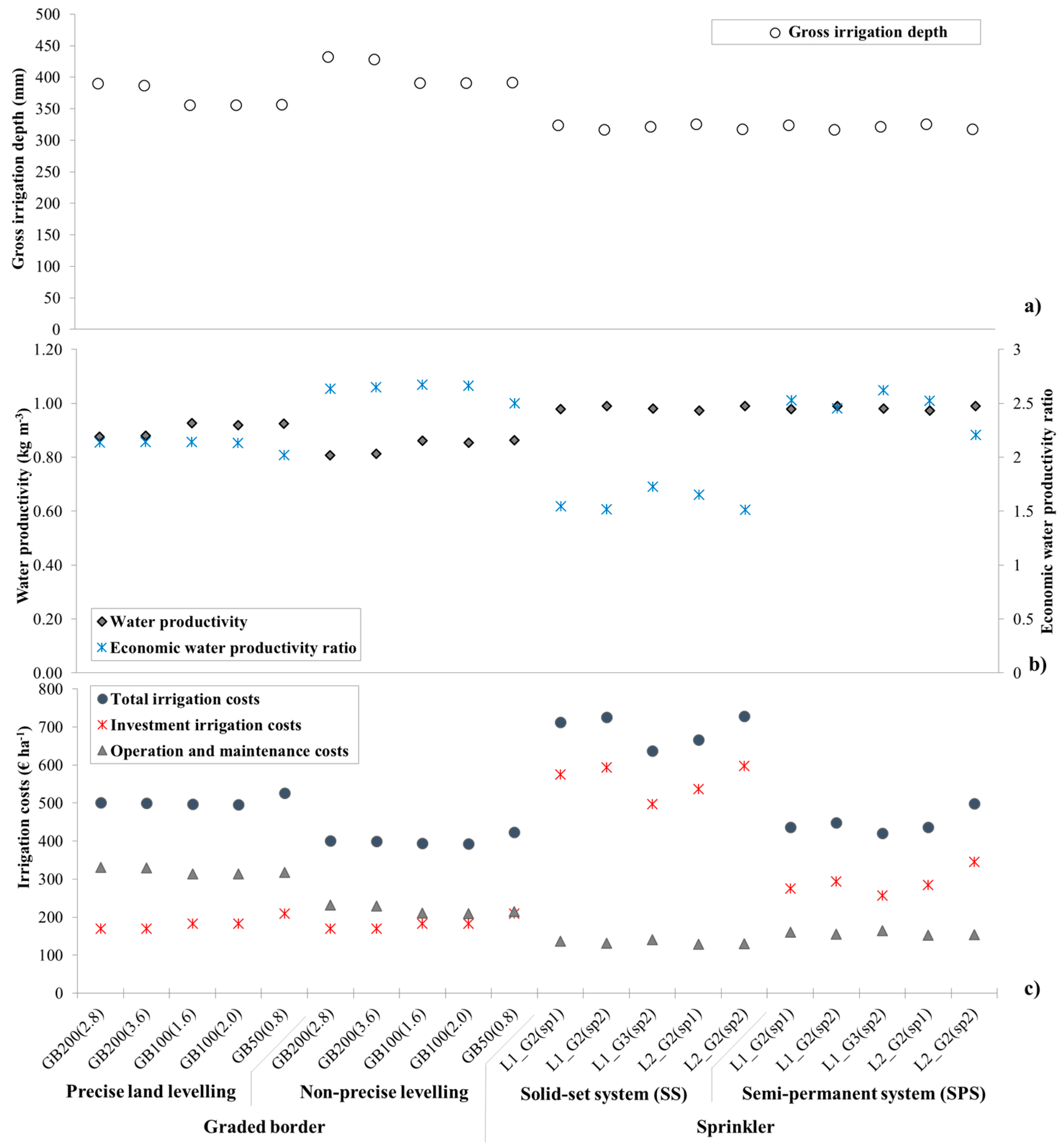
Table 2 shows the results for both strategies and irrigation methods computed for the average year precipitation of 290 mm during the wheat crop season. A leaching fraction of 6% to prevent salt accumulation in the soil profile was considered when calculating the gross irrigation.
To estimate the yield impacts of the various irrigation alternatives, the yield response curve proposed by Solomon [46] was adopted: Ya/Ymax = f(Wa/Wmax), where Ya and Ymax are the actual and the maximum yield (kg·ha−1), Wa is the actual water applied (mm) and Wmax is the water required to achieve Ymax. Related parameters for wheat based on regional data are presented in Table 3 following Kanshaw et al. [15].
Economic input data relative to surface and sprinkler irrigation systems are presented in Table 4. Information about water, labor and yield costs, were obtained from the Ministry of Agriculture and Agrarian Reforms [47].
Information regarding land levelling was provided by the local farmers. The cost for the irrigation equipment, namely the sprinklers and the pipes, were obtained from Senninger® (Claremont, FL, USA) and Maïs Irrigation Co. (Amman, Jordan). The operation and maintenance costs relative to energy, labor and water were updated considering a 4% rate during a 10-year period.

2.3. Application of Multi-Criteria Analysis for the Selection of Alternative Designs

The criteria adopted for ranking alternatives with MCA refer to the attributes presented in Table 5 that follow those previously used by Darouich et al. [23,24]. The indicators used to define the criteria referring to water saving [46] include total irrigation water use (IWU, mm), beneficial water use fraction (BWUF, non-dimensional), non-beneficial water use (NBWU, mm) and water productivity (WP, kg·m−3). IWU corresponds to the season gross irrigation depth (GID). BWUF corresponds to the application efficiency in the SIRMOD model [40] and to Epa (Equation (2)) in sprinkler irrigation. NBWU includes percolation through the bottom of the root zone, runoff and losses by evaporation and wind drift in sprinkling. WP was computed as the ratio between actual yield and total water use (TWU), where TWU is the sum of the infiltrated rainfall, the gross irrigation, thus including the leaching fraction and the seasonal variation of the soil water storage. In agreement with previous studies [48,49], WP is analyzed together with other performance indicators. Indicators relative to the economic criteria [24,49] consist of economic land productivity (ELP, €·ha−1), economic water productivity (EWP, €·m−3), irrigation investment costs per unit of land (IIC, €·ha−1), operation and maintenance costs per unit of land (OMC, €·ha−1) and economic water productivity ratio (EWPR, non-dimensional). ELP is the monetary yield value obtained per unit of land, and EWP is the monetary yield value per unit of water used. EWPR is the ratio of total yield value to the total irrigation cost [49]. As for previous studies (e.g., [23,24,33]), the overlapping or redundancy of criteria was checked and definitely avoided.
The utility functions that enable comparing attributes that have different units are also listed in Table 5. The utilities Uj relative to any criterion j were normalized into the [0–1] interval, with zero for the more adverse and 1 for the most advantageous result. Following previous studies [30,40] where composite programming and ELECTRE II (Elimination Et Choice Translating Reality) were used, considering the required easiness of discussing the results with the irrigation stakeholders, linear utility functions were adopted [23,24,31]:
U j ( x j ) = α   x j + β
where xj is the attribute value relative to criterion j, α is the slope, negative for costs and positive for benefits, and β is the utility value for a null value of the attribute.
The linear weighted sum method [27,50] was adopted to rank the various alternatives because it has been successful used in previous applications [23,24]. It is an aggregative and full compensatory method that leads to a unique global criterion. The high simplicity of this method is a major advantage. For each alternative, the method computes a global utility that represents its integrative score performance:
U = j = 1 Nc λ j U j
where U is the global utility; Nc is the number of criteria; λj is the weight assigned to the criterion j. λj represents the relative importance of a given criterion from the perspective of the decision maker. Criterion weights depend on several factors, including socio-cultural values and economic and/or environmental perspectives. 
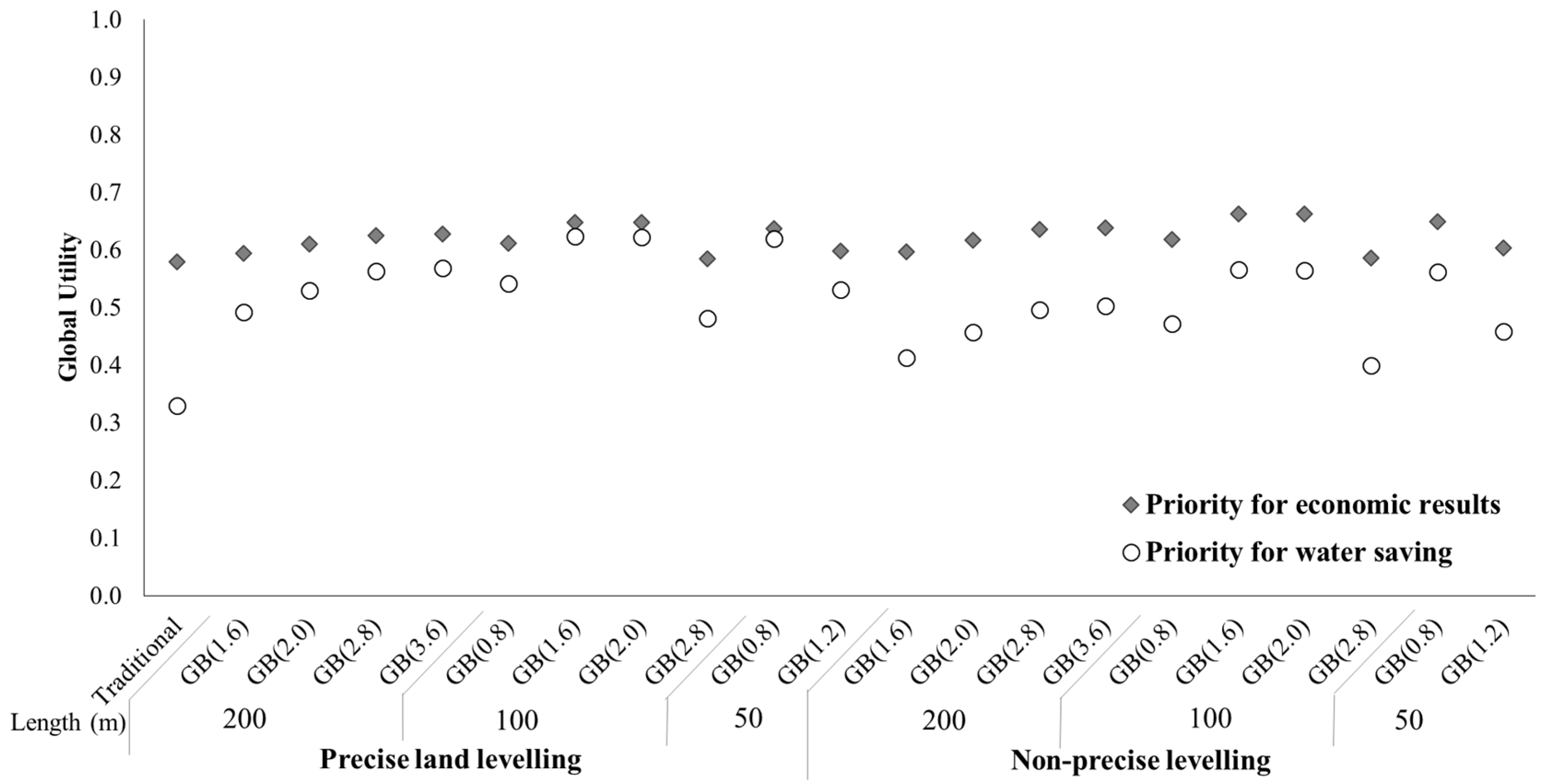
Table 5 presents the weights assigned to attributes for water saving and economic result priorities used to later compare global utilities and building the prioritization scenarios Sc1–Sc5. Several combinations of weights were then used to build those scenarios, starting when 90% of weights were assigned to farm economic results and 10% to water saving (Sc1) and ending with a scenario where 90% of weights were assigned to water saving and 10% to economic results (Sc5). The weights used for the criteria attributes when building the scenarios were proportional to those presented in Table 5. MCA was applied in two steps: first, surface and sprinkler irrigation alternatives were ranked independently; then, they were compared and ranked jointly. Rankings were analyzed for mild and moderate-deficit irrigation.

3. Results

3.1. Economic and Water Saving Performance of Surface Irrigation Alternatives for the Mild-Deficit Strategy

A set of 20 border alternatives was simulated considering various lengths and inflow discharges as described in Section 2.2 and options on land levelling, i.e., precise and non-precise land levelling (PL and NPL). Results in Figure 5 show that adopting PL and lay-flat tubing for water distribution to the borders leads to improving the water use performance relative to present traditional systems.
IWU or GID values obtained for the PL alternatives (Figure 5a) varied from 358 to 439 mm, about 10% less than for NPL alternatives, which ranged from 392 to 494 mm. IWU, as well as BWUF (Figure 5a) depend on the inflow rate together with the basin length (L, m). The best inflow rates are 0.8 L·s−1·m−1 for L = 50 m, 1.6–2.0 L·s−1·m−1 for L = 100 m and 2.8–3.6 L·s−1·m−1 for L = 200 m (Figure 5a,b). BWUF ranged from 0.49 to 0.61 for NPL alternatives and 0.55–0.67 in the case of precise levelling (Figure 5b), with lower values for long borders (L = 200 m) and higher values for L = 100 m. The BWUF values obtained are similar to those reported for cotton [23]. WP values ranged from 0.74 to 0.87 kg·m−3 for NPL and varied from 0.81 to 0.93 kg·m−3 for PL alternatives. These results are in line with other studies, e.g., Oweis and Hachum [17] and Karrou and Oweis [51] in the same region.
Economic results (Figure 5c) show that the investment cost, including relative to initial land levelling, varies with the borders’ length from 170 to 209 €·ha−1, with the smaller value for the 200 length. The annual cost of land levelling maintenance in case of PL alternatives is 122 €·ha−1. The labor and water costs for system operation range from 190 to 260 €·ha−1 with the highest cost for NPL alternatives since the latter require longer application time, thus more labor. Results are in agreement with those reported by Darouich et al. [23] and Rudrapur and Patil [52]. EWPR ranged from 2.3 to 2.7 for NPL and from 1.9 to 2.2 for PL alternatives. This difference is due to higher total irrigation costs associated with precise land levelling. Nevertheless, both alternatives are profitable since EWPR values are always larger than 1.0.
The global utilities (U) characterizing all alternatives when priorities are assigned to water saving or to farm economic returns are presented in Figure 6. Results show that when the priority is assigned to farm economics, the U values are always superior to the ones relative to water saving prioritization. Moreover, related U values for NPL alternatives are slightly larger than for precise levelling, while when water saving is considered as the priority, the U values for PL are superior. Utility values, when the priority, assigned to economic returns range from 0.58 to 0.66. As expected, traditional irrigation presents the lowest U value in terms of water saving, while for economics (U = 0.58), it is similar to those obtained for a 100-m graded border with a large flow rate of 2.8 L·s−1·m−1, for both NPL and PL.

3.2. Economic and Water Saving Performance of Sprinkler Irrigation Alternatives for the Mild-Deficit Strategy

A set of sprinkler alternatives was compared. GID vary little among these alternatives, from 319 to 327 mm, because the design constraints were similar. Computations with PROASPER (Equation (2)) produced DEpa values ranging from 84.1% to 87.8% when pa = 75%. CU ranged from 80.9% to 85.3%, and Re values varied from 0.92 to 0.93 when ET was 4.5 mm·day−1 and wind speed was 3.5 m·s−1. Computed values for Epa resulted in the range 77.0%–80.3%.
Figure 7 shows that differences between SS and SPS systems are mainly due to the investment irrigation costs (IIC). The investment cost required for SS (496–666 €·ha−1) is about double that for SPS (255–346 €·ha−1). The main factors affecting IIC for both types of systems refer to layouts and the number and type of sprinklers, including the nominal discharge (Table 1). Contrary to IIC, the operation and maintenance costs (OMC) were slightly higher for SPS (152–180 €·ha−1) than those for SS (124–151 €·ha−1) (Figure 7) due to higher labor requirements (Table 4). The variation of OMCs between layouts and sprinklers types mainly relate to the required head pressure.
The global utilities (U) relative to the sprinkler alternatives when priorities are assigned to water saving or economic returns are compared in Figure 8. Differences referring to water saving are very small, but when considering economic results, there is evidence of the better performance by the semi-permanent systems due to lower total costs (Figure 7). The best ranked alternative refers to a SPS system using layout L1 with sprinkler sp2 and a spacing of 15 m × 12 m.

3.3. Comparing Sprinkler and Surface Irrigation Alternatives

Results when mild-deficit irrigation is adopted show that sprinkler irrigation systems can lead to lower GID (Figure 9a), due to higher BWUF, resulting in water savings varying from 11% to 34% relative to surface irrigation; BWUF is nearly 0.80 for sprinkler systems and varies from 0.49 to 0.67 for GB. Since GID is smaller for sprinkler systems, assuming that yields are similar for both surface and sprinkler systems, it results in larger water productivity (WP of 0.97–0.99 kg·m−3) for the latter (Figure 9b). However, the EWPR for solid set systems are quite low (1.4–1.7) because those sprinkler systems require higher investment cost than surface irrigation. Border irrigation presents higher EWPR than SS despite having higher labor and water costs, as well as land levelling maintenance costs for the case of precise levelling (Figure 9c). Because high pressure sprinklers were rejected in the previous step of selecting alternatives, the energy cost for the sprinkler systems is relatively low, 18%–29% of the operational costs. However, the total irrigation costs for sprinkler systems resulted in being 8%–31% higher than for surface systems (Figure 9c).
Global utilities for the best alternatives of SS and SPS are compared with those for precise and non-precise levelled GB in Figure 10. Results show that when the priority is assigned to water saving, sprinkler systems perform better than surface irrigation. The worst results were obtained for the long borders (200 m) without precise levelling. In terms of economic returns, the best results are for sprinkler-SPS alternatives, while solid sets have worse results due to high investment costs. In economic terms, GB alternatives perform similarly to solid sets.
The ranking of the retained alternatives for both sprinkler and surface irrigation when mild-deficit strategy is adopted is presented in Table 6 for various prioritization scenarios (Sc) built with weights proportional to those in Table 5. Since priorities are assigned through selecting appropriate weights (λ, Equation (3)) several combinations were considered, Sc1–Sc5. As referred in Section 2.3, in Sc1, 90% of weights were assigned to economic results, while only 10% of weights were for water saving, while for Sc5, only 20% of weights were assigned to economic returns and 80% to water saving. Sc2, 3 and 4 are intermediate scenarios with weights for economic results decreasing (respectively 80%, 70%, 50%) and those for water saving increasing (respectively 20%, 30%, 50%).
Results in Table 6 clearly show that SPS are selected first for all scenarios. The best option for all scenarios is layout L1 (Figure 4) with sp2 (Table 1). Sprinkler spacing G3 (12 m × 15 m) is the best option for Scenarios 1–4. For Sc5, the best system is similar, but with a smaller spacing of 12 m × 12 m. Graded borders with a 100-m length rank better when the highest weights are assigned to economic return (Sc1, Sc2 and Sc3). Contrarily, they only show a ranking of 11 when at least 50% of weights are assigned to water saving (Sc4 and Sc5). These results indicate that border irrigation, in spite of presenting a good ranking when considering the economic returns, is not an easy to implement solution for wheat irrigation where land is sloping.
Comparing the alternatives in terms of water use and productivity indicators (Table 7) and taking into consideration the water-yield response curve of Table 3, it can be observed that: gross irrigation depth (GID) is higher for GB; the beneficial water use fraction (BWUF) is higher for sprinkler systems; while water productivity (WP), economic WP (EWP) and economic land productivity (ELP) are also higher for sprinkler systems. EWPR present better values for GB than for sprinkler systems. However, considering the results previously obtained for cotton in the same area [23], graded borders may be a solution when wheat is in rotation with cotton, since sprinkler irrigation may negatively impact cotton fiber quality.
Moderate-deficit irrigation resulted in a net irrigation depth reduced by 25% relative to mild-deficit irrigation (Table 2), thus in a reduction of the total water use and of GID (Table 7). Small reductions in ELP and EWPR were found due to the decreased yields.
Ranking the various alternatives regarding the irrigation strategies, it can be observed (Table 8) that mild-deficit irrigation ranks before moderate-deficit irrigation for Sc1 and Sc2, for which the weights assigned to economic returns are higher. For the remaining scenarios, MoD ranks first regardless of the irrigation system. Graded border alternatives regularly rank after the sprinkler SPS ones. It may be concluded that moderate-deficit irrigation produced satisfactory results in terms of WP, EWP and EWPR and consists of a convenient option for irrigation management in water-scarce environments, as for the present case study. Nevertheless, full economic analysis is required in future studies.

4. Conclusions

Multi-criteria analysis was applied to select alternative systems for supplemental irrigation of wheat in northeastern Syria. Graded borders, with and without precise land levelling, and solid-set and semi-permanent sprinkler systems were considered. The first were designed and selected with the SADREG model, and the latter were designed with the PROASPER model. Alternatives for both types of systems were compared and ranked using MCA for diverse scenarios of water saving and farm economic return prioritization. The use of MCA was revealed to be appropriate for both selecting design irrigation system alternatives and for selecting among all alternatives when both type of systems were considered.
Alternatives with precise land levelling resulted in being better when water saving was the aim due to a better controlled advance time and, thus, reduced percolation. Relative to sprinkler systems, the best results were for semi-permanent ones because investment costs were smaller than for solid set systems, and there were small differences in terms of water use and saving between both types of sprinkler systems. Comparing surface and sprinkler systems together, the global utility for the semi-permanent systems ranked better independent of the prioritization. These results were likely due to higher water use and costs of land levelling in the case of graded borders. When moderate-deficit irrigation was considered, ranking was only slightly modified. Graded borders ranked regularly after sprinkler systems likely because land in Ras-El-Ain is not flat, but gently undulated. However, surface irrigation is feasible for wheat when in rotation with cotton.
The outcomes of this study using MCA have two types of implications. The first refer to the need for appropriately carefully considering water use and saving, contrasting with economic results. Most studies comparing irrigation systems just focus on water use and saving or, less frequently, on economic results. This study, as previous ones [23,24], shows that using appropriate field data, modelling and MCA, it is possible to advance and innovate in the domain of selecting farm irrigation systems considering a wide range of water use performance and economic criteria. The second type of implications consists of developing the appropriate incentives and farmers’ training that may contribute to implementing innovations at the farm. This is particularly challenging for northeastern Syria after peace is achieved, as strongly desired by the population.
Meanwhile, further studies should focus on the effect of farm size and of the natural land gradient on selecting the farm irrigation systems since they influence investment costs in addition to the factors considered in the current study. Knowing the current war conditions in the area under study, a strong word of hope has to be clearly added to these conclusions.

Acknowledgments

The authors thank Centre International De Hautes Études Agronomiques Méditerranéennes/Institut Agronomique Méditerranéen (CIHEAM/IAM), Bari, Italy, and the Italian Cooperation Agency, Rome, for funding the field study. Modelling studies were partly funded by the project PTDC/AGR-AAM/105432/2008, Foundation for Science and Technology (FCT), Portugal. The first author has been recipient of a FCT fellowship SFRH/BD/60516/2009. The fourth author thanks the postdoctoral fellowship (SFRH/BPD/102478/2014) provided by FCT. The support of FCT through the research unit LEAF-Linking Landscape, Environment, Agriculture and Food (UID/AGR/04129/2013) is also acknowledged. Support by Gonçalo C. Rodrigues is also acknowledged.

Author Contributions

Hanaa Darouich and Luis S. Pereira conceived of and designed the experiments. The first author performed the field experiments under supervision of the fifth author. The first author together with Maria R. Cameira; José M. Gonçalves and Paula Paredes authors analyzed the data. The first author wrote the paper; and all of the other authors contributed to its revision.

Conflicts of Interest

The authors declare no conflict of interest.

Abbreviations

Symbols
BWUFbeneficial water use fraction (ratio)
CUcoefficient of uniformity (%)
DEpadistribution efficiency when the area adequately irrigated is pa (%)
ETc actactual evapotranspiration (mm)
ELPeconomic land productivity (€·ha−1)
Epadesign application efficiency when the area adequately irrigated is pa (%)
ETocrop reference evapotranspiration (mm)
EWPeconomic water productivity (€·m−3)
EWPReconomic water productivity ratio (ratio)
GIDgross irrigation depth (mm)
IICinvestment irrigation costs (€·ha−1)
IWUirrigation water use (m3·ha−1)
NBWUnon-beneficial water use (mm)
Oeeffective fraction of water discharged (decimal)
OMCoperation and maintenance cost (€·ha−1)
pdepletion fraction for no stress (dimensionless)
papercentage of area adequately irrigated (%)
Reeffective fraction of water applied (decimal)
TWUtotal water use (mm)
Uglobal utility (dimensionless)
Ujutility relative to criterion j (dimensionless)
Wanet applied water to achieve the actual yield Ya (mm)
Wmaxnet applied water to achieve the maximum yield Ymax (mm)
WPwater productivity (kg·m−3)
xiattributes of criteria i
Yaactual yield (kg·ha−1)
Ymaxmaximum (potential) yield (kg·ha−1)
Zcumulative infiltration (m3·m−1)
αparameter of the Ui equation (dimensionless)
βutility value for a null value of the attribute (dimensionless)
λjweight assigned to criterion i
τinfiltration opportunity time (min)
Abbreviations
G1, 2, … 5sprinkler spacing
GBgraded border
L1, L2layout’s type, 1 and 2
MADmanagement allowed depletion
MCAmulticriteria analysis
MDmild-deficit irrigation
MoDmoderate-deficit irrigation
Ncnumber of criteria
NPLnon-precise land levelling
PEpolyethylene
PLprecise land levelling
PVCpolyvinyl chloride
Sc1, 2, …, 5Scenarios 1, 2, …, 5
sp1, 2, …, 4Sprinkler Types 1, 2, …, 4
SPSsemi-permanent system (gridded-pipe)
SSsolid-set system

References

  1. Araus, J.L.; Ferrio, J.P.; Buxo, R.; Voltas, J. The historical perspective of dryland agriculture: Lessons learned from 10,000 years of wheat cultivation. J. Exp. Bot. 2007, 58, 131–145. [Google Scholar] [CrossRef] [PubMed]
  2. Sadiddin, A.; Atiya, B. Analysis of Agricultural Production for Selected Crops: Wheat, Cotton and Barley; Working Paper No. 44; National Agricultural Policy Centre (NAPC): Damascus, Syria, 2009; 50p. [Google Scholar]
  3. Beaumont, P. Agricultural and environmental changes in the upper Euphrates catchment of Turkey and Syria and their political and economic implications. Appl. Geogr. 1996, 16, 137–157. [Google Scholar] [CrossRef]
  4. Hole, F. Drivers of unsustainable land use in the semi-arid Khabur River Basin, Syria. Geogr. J. 2009, 47, 4–14. [Google Scholar] [CrossRef]
  5. Öztan, M.; Axelrod, M. Sustainable transboundary groundwater management under shifting political scenarios: The Ceylanpinar Aquifer and Turkey–Syria relations. Water Int. 2011, 36, 671–685. [Google Scholar] [CrossRef]
  6. Mourad, K.A.; Berndtsson, R. Water Status in the Syrian Water Basins. Open J. Mod. Hydrol. 2012, 2, 15–20. [Google Scholar] [CrossRef]
  7. Aw-Hassan, A.; Rida, F.; Telleria, R.; Bruggeman, A. The impact of food and agricultural policies on groundwater use in Syria. J. Hydrol. 2014, 513, 204–215. [Google Scholar] [CrossRef]
  8. Ibrahim, B. Climate change effects on agriculture and water resources availability in Syria. In Implementing Adaptation Strategies by Legal, Economic and Planning Instruments on Climate Change; Albrecht, E., Schmidt, M., Mißler-Behr, M., Spyra, S.P.N., Eds.; Springer: Berlin/Heidelberg, Germany, 2014; pp. 305–313. [Google Scholar]
  9. Yigezu, Y.A.; Ahmed, M.A.; Shideed, K.; Aw-Hassan, A.; El-Shater, T.; Al-Atwan, S. Implications of a shift in irrigation technology on resource use efficiency: A Syrian case. Agric. Syst. 2013, 118, 14–22. [Google Scholar] [CrossRef]
  10. Yigezu, Y.A.; Aw-Hassan, A.; Shideed, K.; Sommer, R.; El-Shater, T. A policy option for valuing irrigation water in the dry areas. Water Policy 2014, 16, 520–535. [Google Scholar] [CrossRef]
  11. Sadiddin, A. An assessment of policy impact on agricultural water use in the northeast of Syria. Environ. Manag. Sustain. Dev. 2013, 2, 74–105. [Google Scholar] [CrossRef]
  12. Zhang, H.; Oweis, T. Water–yield relations and optimal irrigation scheduling of wheat in the Mediterranean region. Agric. Water Manag. 1999, 38, 195–211. [Google Scholar] [CrossRef]
  13. Oweis, T.; Rodrigues, P.N.; Pereira, L.S. Simulation of supplemental irrigation strategies for wheat in Near East to cope with water scarcity. In Tools for Drought Mitigation in Mediterranean Regions; Rossi, G., Cancelliere, A., Pereira, L.S., Oweis, T., Shatanawi, M., Zairi, A., Eds.; Kluwer: Dordrecht, The Netherlands, 2003; pp. 259–272. [Google Scholar]
  14. Somme, G.; Oweis, T.Y.; El Omar, F.; Hachum, H.; Shayeb, R.; Jooni, N. Rainfed Wheat Productivity with Supplemental Irrigation in Al-Hasakeh, Northern Syria. On-Farm Water Husbandry in WANA; Research Report No 4; International Center for Agricultural Research in the Dry Areas (ICARDA): Aleppo, Syria, 2005. [Google Scholar]
  15. Kanshaw, I.; Kheeti, M.; Al-Shawwa, F. Impact of supplementary irrigation on production of durum wheat (Triticum durum L.) in Quneitra Governorate. J. Agric. Sci. 2007, 22, 353–378. (In Arabic) [Google Scholar]
  16. Oweis, T.; Hachum, A. Water harvesting and supplemental irrigation for improved water productivity of dry farming systems in West Asia and North Africa. Agric. Water Manag. 2006, 80, 57–73. [Google Scholar] [CrossRef]
  17. Oweis, T.; Hachum, A. Optimizing supplemental irrigation: Tradeoffs between profitability and sustainability. Agric. Water Manag. 2009, 96, 511–516. [Google Scholar] [CrossRef]
  18. Zairi, A.; El Amami, H.; Slatni, A.; Pereira, L.S.; Rodrigues, P.N.; Machado, T. Coping with drought: Deficit irrigation strategies for cereals and field horticultural crops in Central Tunisia. In Tools for Drought Mitigation in Mediterranean Regions; Rossi, G., Cancelliere, A., Pereira, L.S., Oweis, T., Shatanawi, M., Zairi, A., Eds.; Kluwer Academic Publishers: Dordrecht, The Netherlands, 2003; pp. 181–201. [Google Scholar]
  19. Karam, F.; Kabalan, R.; Breidi, J.; Rouphael, Y.; Oweis, T. Yield and water-production functions of two durum wheat cultivars grown under different irrigation and nitrogen regimes. Agric. Water Manag. 2009, 96, 603–615. [Google Scholar] [CrossRef]
  20. Bonfil, D.J.; Karnieli, A.; Raz, M.; Mufradi, I.; Asido, S.; Egozi, H.; Hoffman, A.; Schmilovitch, Z. Decision support system for improving wheat grain quality in the Mediterranean area of Israel. Field Crops Res. 2004, 89, 153–163. [Google Scholar] [CrossRef]
  21. Saadi, S.; Todorovic, M.; Tanasijevic, L.; Pereira, L.S.; Pizzigalli, C.; Lionello, P. Climate change and Mediterranean agriculture: Impacts on winter wheat and tomato crop evapotranspiration, irrigation requirements and yield. Agric. Water Manag. 2015, 147, 103–115. [Google Scholar] [CrossRef]
  22. Pereira, L.S.; Oweis, T.; Zairi, A. Irrigation management under water scarcity. Agric. Water Manag. 2002, 57, 175–206. [Google Scholar] [CrossRef]
  23. Darouich, H.; Gonçalves, J.M.; Muga, A.; Pereira, L.S. Water saving vs. farm economics in cotton surface irrigation: An application of multicriteria analysis. Agric. Water Manag. 2012, 115, 223–231. [Google Scholar] [CrossRef]
  24. Darouich, H.; Pedras, C.M.G.; Gonçalves, J.M.; Pereira, L.S. Drip vs. surface irrigation: A comparison focusing water saving and economic returns using multicriteria analysis applied to cotton. Biosyst. Eng. 2014, 122, 74–90. [Google Scholar] [CrossRef]
  25. Lecina, S.; Isidoro, D.; Playán, E.; Aragüés, R. Irrigation modernization and water conservation in Spain: The case of Riegos del Alto Aragón. Agric. Water Manag. 2010, 97, 1663–1675. [Google Scholar] [CrossRef]
  26. Pomerol, J.C.; Barba-Romero, S. Multicriterion Decision in Management: Principles and Practice; Series 25; Kluwer Acad. Publ.: Dordrecht, The Netherlands, 2000. [Google Scholar]
  27. Ishizaka, A.; Nemery, P. Multi-Criteria Decision Analysis: Methods and Software; John Wiley and Sons Inc.: Hoboken, NJ, USA, 2013; ISBN 978-1-1199-7407-9. [Google Scholar]
  28. Rinaldi, M.; He, Z. Decision support systems to manage irrigation in agriculture. Adv. Agron. 2014, 123, 229–279. [Google Scholar]
  29. Tuo, Y.; Chiogna, G.; Disse, M. A Multi-criteria model selection protocol for practical applications to nutrient transport at the catchment scale. Water 2015, 7, 2851–2880. [Google Scholar] [CrossRef]
  30. Pedras, C.M.G.; Pereira, L.S. Multicriteria analysis for design of microirrigation systems. Application and sensitivity analysis. Agric. Water Manag. 2009, 96, 702–710. [Google Scholar] [CrossRef]
  31. Gonçalves, J.M.; Muga, A.P.; Horst, M.G.; Pereira, L.S. Furrow irrigation design with multicriteria analysis. Biosyst. Eng. 2011, 109, 266–275. [Google Scholar] [CrossRef]
  32. Monaco, F.; Sali, G.; Ben Hassen, M.; Facchi, A.; Romani, M.; Valè, G. Water management options for rice cultivation in a temperate area: A multi-objective model to explore economic and water saving results. Water 2016, 8, 336. [Google Scholar] [CrossRef]
  33. Rodrigues, G.C.; Paredes, P.; Gonçalves, J.M.; Alves, I.; Pereira, L.S. Comparing sprinkler and drip irrigation systems for full and deficit irrigated maize using multicriteria analysis and simulation modelling: Ranking for water saving vs. farm economic returns. Agric. Water Manag. 2013, 126, 85–96. [Google Scholar] [CrossRef]
  34. Holzapfel, E.; Mariño, M.; Chavez-Morales, J. Procedure to select an optimum irrigation method. J. Irrig. Drain. Eng. 1985, 111, 319–329. [Google Scholar] [CrossRef]
  35. Trout, T.J.; Kincaid, D.C.; Westermann, D.T. Comparison of Russet Burbank yield and quality under furrow and sprinkler irrigation. Am. Potato J. 1994, 71, 15–28. [Google Scholar] [CrossRef]
  36. O’Neill, C.J.; Humphreys, E.; Louis, J.; Katupitiya, A. Maize productivity in southern New South Wales under furrow and pressurised irrigation. Anim. Prod. Sci. 2008, 48, 285–295. [Google Scholar] [CrossRef]
  37. Albaji, M.; Shahnazari, A.; Behzad, M.; Naseri, A.; BoroomandNasab, S.; Golabi, M. Comparison of different irrigation methods based on the parametric evaluation approach in Dosalegh plain: Iran. Agric. Water Manag. 2010, 97, 1093–1098. [Google Scholar] [CrossRef]
  38. Montazar, A.; Behbahani, S.M. Development of an optimised irrigation system selection model using analytical hierarchy process. Biosyst. Eng. 2007, 98, 155–165. [Google Scholar] [CrossRef]
  39. Allen, R.G.; Pereira, L.S.; Raes, D.; Smith, M. Crop Evapotranspiration. Guidelines for Computing Crop Water Requirements; FAO Irrigation and Drainage Paper 56; Food and Agriculture Organization: Rome, Italy, 1998; p. 300. [Google Scholar]
  40. Gonçalves, J.M.; Pereira, L.S. Decision support system for surface irrigation design. J. Irrig. Drain. Eng. 2009, 135, 343–356. [Google Scholar] [CrossRef]
  41. Rodrigues, G.C.; Sequeira, B.; Paredes, P.; Pereira, L.S. PROASPER, um SAD para projeto de sistemas de rega por aspersão. In Tecnologias para o Uso Sustentável da Água em Rega; Pereira, L.S., Victória, F.R.B., Paredes, P., Garcia, M., Palácios, E., Torrecillas, A., Eds.; Edições Colibri e CEER: Lisbon, Portugal, 2010; pp. 15–19. (In Portuguese) [Google Scholar]
  42. Walker, W.R. SIRMOD–Surface Irrigation Modeling Software; Utah State University: Logan, VT, USA, 1998. [Google Scholar]
  43. Keller, J.; Bliesner, R.D. Sprinkle and Trickle Irrigation; Van Nostrand Reinhold, Chapman and Hall: New York, NY, USA, 1990. [Google Scholar]
  44. Liu, Y.; Teixeira, J.L.; Zhang, H.J.; Pereira, L.S. Model validation and crop coefficients for irrigation scheduling in the North China Plain. Agric. Water Manag. 1998, 36, 233–246. [Google Scholar] [CrossRef]
  45. Pereira, L.S.; Teodoro, P.R.; Rodrigues, P.N.; Teixeira, J.L. Irrigation scheduling simulation: The model ISAREG. In Tools for Drought Mitigation in Mediterranean Regions; Rossi, G., Cancelliere, A., Pereira, L.S., Oweis, T., Shatanawi, M., Zairi, A., Eds.; Kluwer: Dordrecht, The Netherlands, 2003; pp. 161–180. [Google Scholar]
  46. Solomon, K.H. Yield related interpretations of irrigation uniformity and efficiency measures. Irrig. Sci. 1984, 5, 161–172. [Google Scholar] [CrossRef]
  47. Ministry of Agriculture and Agrarian Reform (MAAR). Land Use Balance; Department of Statistics and Planning, Ministry of Agriculture and Agrarian Reform: Damascus, Syria, 2011. (In Arabic)
  48. Wichelns, D. Do estimates of water productivity enhance understanding of farm-level water management? Water 2014, 6, 778–795. [Google Scholar] [CrossRef]
  49. Pereira, L.S.; Cordery, I.; Iacovides, I. Improved indicators of water use performance and productivity for sustainable water conservation and saving. Agric. Water Manag. 2012, 108, 39–51. [Google Scholar] [CrossRef]
  50. Stanimirovic, I.P.; Zlatanovic, M.L.; Petkovic, M.D. On the linear weighted sum method for multi-objective optimization. Facta Acta Univ. 2011, 26, 49–63. [Google Scholar]
  51. Karrou, M.; Oweis, T. Water and land productivities of wheat and food legumes with deficit supplemental irrigation in a Mediterranean environment. Agric. Water Manag. 2012, 107, 94–103. [Google Scholar] [CrossRef]
  52. Rudrapur, S.; Patil, B.L. Impact of border strip and flood method of irrigation on wheat cultivation in the Malaprabha Command Area of Karnataka. J. Agric. Stud. 2015, 3, 212–218. [Google Scholar] [CrossRef]
Figure 1. Average monthly rainfall, reference evapotranspiration (ETo) and maximum and minimum temperature at Ras-El-Ain (1993–2002).
Water 09 00050 g001
Figure 2. Schematic flow-chart of SADREG for multilevel approach for the design and application of multi-criteria ranking and selection [40].
Water 09 00050 g002
Figure 3. Functional diagram of the PROASPER model.
Water 09 00050 g003
Figure 4. Schematic drawing of two alternative pipe layouts. (a) Layout 1; (b) Layout 2.
Water 09 00050 g004
Figure 5. Comparing design alternatives for graded borders (GB) relative to: (a) beneficial water use fraction; (b) gross irrigation, runoff and deep percolation (mm); and (c) irrigation costs (€·ha−1). Values inside brackets refer to inflow rates (L·s−1·m−1).
Water 09 00050 g005
Figure 6. Global utility value for graded borders when the priority is assigned to economic results or to water saving. The value in brackets represents inflow rates (L·s−1 m−1).
Water 09 00050 g006
Figure 7. Comparing solid set and semi-permanent sprinkler system alternatives for total, investment and operation and maintenance irrigation costs (€·ha−1). Layouts are defined in Figure 4, while sprinkler spacing (G1, 2, …, 5) and sprinkler types (sp1, 2, …, 4) are identified in Table 1.
Water 09 00050 g007
Figure 8. Global utility values relative to solid set and semi-permanent sprinkler systems when the priority is assigned to water saving or to economic results. Layouts are defined in Figure 4, and sprinkler spacing (G1, 2, …, 5) and sprinkler types (sp1, 2, …, 4) are identified in Table 1.
Water 09 00050 g008
Figure 9. Comparing borders and sprinkler irrigation alternatives for: (a) gross irrigation depth, GID (mm); (b) water productivity, WP (kg·m−3) and economic water productivity ratio, EWPR; and (c) irrigation costs (€·ha−1). Border lengths are of 50, 100 and 200 m, and inflow rates (L·s−1·m−1) are in brackets. Sprinklers refer to layouts L1 and L2; spacings are G2 and G3; and sprinkler types are sp1 and sp2.
Water 09 00050 g009
Figure 10. Comparing global utilities for sprinkler solid-set and semi-permanent systems with those for precise and non-precise levelled graded borders when priority is assigned to water saving or to economic returns. Sprinkler systems refer to layouts L1 and L2, spacings G2 and G3 and sprinklers sp1 and sp2. Graded borders have 50-, 100- and 200-m lengths and inflow rates from 0.8 to 3.6 L·s−1·m−1.
Water 09 00050 g010
Table 1. Characteristics of sprinklers used for the various alternatives and respective application rate for various sprinkler spacing.
Sprinklerssp1sp2sp3sp4
Nozzle’s diameter (mm)2.383.183.973.97
Flow rate (m3·h−1)0.300.550.871.11
Pressure head (m)25272745
Jet throw (m)11.313.114.115.2
Price (€ per sprinkler)13131718
Life time (years)5555
Sprinkler spacing (m × m)9 × 12 (G1)12 × 12 (G2)12 × 12 (G2)12 × 15 (G3)15 × 15 (G4)15 × 18 (G5)
Application rate (mm·h−1)2.782.083.823.063.874.09
Table 2. Wheat irrigation scheduling for surface and sprinkler systems at Ras-El-Ain considering mild (MD) and moderate-deficit (MoD) irrigation.
Irrigation MethodIrrigation StrategyNumber of Irrigation EventsNet Irrigation Depth (mm)ETc act (mm)Effective Rainfall (mm)
Per EventPer Season
TraditionalTraditional365–87195–261413156
BorderMD460240439134
SprinklerMD830240450156
BorderMoD360180410164
SprinklerMoD630180409163
Table 3. Water-yield function parameters.
Wa/Wmax0.250.50.751.01.52.02.5
Ya/Ymax0.0640.360.651.010.950.8
Notes: Ya and Ymax are the actual and the maximum yields that correspond to the net applied water Wa and Wmax, respectively.
Table 4. Labor requirements and unit costs for surface and sprinkler irrigation.
Surface Irrigation
Initial land levellingHourly cost110 €
Operation time per area10.0 h
Precision land levellingHourly cost110 €
Operation time per area3.0 h
Frequency for graded borders3 years
Lay-flat gated pipeDiameters, 12.7, 22.9, 30.5 cm (1-year lifetime)0.15, 0.22, 0.30 € m−1
Lay-flat valve 0.23 € per valve
Labor requirementsEquipment operation (per event)40 min/100 m
Pipe installation60 min/100 m
Pipe removal40 min/100 m
Sprinkler Irrigation
Labor requirements for solid-set systemsSystem installation22 h·ha−1
System repair/replacement2 h·ha−1
System removal9 h·ha−1
System operation0.5 h·ha−1·event−1
Labor requirements for semi-permanent gridded pipe systemsSystem installation20 h·ha−1
System repair/replacement2 h·ha−1
System removal9 h·ha−1
System operation5 h·ha−1·event−1
PE pipes (6 bar and 5-year lifetime)Diameters 50, 63, 75 mm0.56, 0.83, 1.20 €·m−1
Diameters 90, 110, 125 mm1.73, 2.52, 3.24 €·m−1
PVC pipes (4 bar and 10-year lifetime)Diameters 75, 110, 125 mm0.82, 1.48, 1.89 €·m−1
Diameters 90, 110, 125 mm1.44, 2.11, 2.89 €·m−1
Financial Data and Prices (Common to both Systems)
Analysis period10 years
Annual interest rate4%
Water price0.022 €·m−3
Labor cost0.8 €·h−1
Yield price0.21 €·kg−1
Electric power0.08 €·kWh
Table 5. Criteria attributes, utility functions and weights used to compare global utilities and to build prioritization scenarios.
Criteria Attributes (x)SymbolUnitsUtility FunctionsWeights (λ, %) Assigned to Attributes When Prioritizing
Water SavingEconomic Results
Economic productivity and costs2080
Economic land productivityELP€·ha−1U(x) = 0.907 × 10−3x515
Economic water productivityEWP€·m−3U(x) = 4.0x415
Economic water productivity ratioEWPRratioU(x) = 0.1667x520
Irrigation investment costsIIC€·ha−1U(x) = 1 − 1.43 × 10−3x315
Operation and maintenance costsOMC€·ha−1U(x) = 1 − 1.43 × 10−3x315
Water saving and environment8020
Irrigation water useIWUmmU(x) = 1 − 1.8 × 10−3x205
Beneficial water use fractionBWUFratioU(x) = 1.0x205
Water productivityWPkg·m−3U(x) = 0.833x205
Non-beneficial water useNBWUmmU(x) = 1 − 3.57 × 10−2x205
Table 6. Ranking of best alternatives depending on the priorities assigned for various scenarios where weights for water saving change from Sc1 (higher weights for economic results) through Sc5 (higher weights to water savings) when mild-deficit irrigation is adopted for the sprinkler vs. graded border alternatives (shaded).
Sc1 (10–90)Sc2 (20–80) aSc3 (30–70)Sc4 (50–50)Sc5 (80–20) a
1SPS_L1_G3(sp2)SPS_L1_G3(sp2)SPS_L1_G3(sp2)SPS_L1_G3(sp2)SPS_L1_G2(sp2)
2SPS_L1_G2(sp1)SPS_L1_G2(sp1)SPS_L1_G2(sp1)SPS_L1_G2(sp2)SPS_L1_G3(sp2)
3SPS_L2_G2(sp1)SPS_L2_G2(sp1)SPS_L1_G2(sp2)SPS_L1_G2(sp1)SPS_L2_G2(sp2)
4SPS_L1_G2(sp2)SPS_L1_G2(sp2)SPS_L2_G2(sp1)SPS_L2_G2(sp1)SPS_L1_G2(sp1)
5GB100NPL(2.0)SPS_L2_G2(sp2)SPS_L2_G2(sp2)SPS_L2_G2(sp2)SS_L1_G2(sp2)
6GB100NPL(1.6)GB100NPL(2.0)GB100NPL(1.6)SS_L1_G3(sp2)SPS_L2_G2(sp1)
7SPS_L2_G2(sp2)GB100NPL(1.6)GB100NPL(2.0)SS_L1_G2(sp2)SS_L1_G3(sp2)
8GB50NPL(0.8)GB50NPL(0.8)GB50NPL(0.8)SS_L2_G2(sp1)SS_L2_G2(sp2)
9GB200NPL(3.6)GB200NPL(3.6)GB100PL(1.6)SS_L1_G2(sp1)SS_L1_G2(sp1)
10GB200NPL(2.8)GB200NPL(2.8)GB100PL(2.0)SS_L2_G2(sp2)SS_L2_G2(sp1)
11GB100PL(2.0)GB100PL(2.0)GB200NPL(3.6)GB100PL(1.6)GB100PL(1.6)
12GB100PL(1.6)GB100PL(1.6)GB50PL(0.8)GB100PL(2.0)GB100PL(2.0)
13GB50PL(0.8)GB50PL(0.8)GB200NPL(2.8)GB50PL(0.8)GB50PL(0.8)
14GB200PL(3.6)SS_L1_G3(sp2)SS_L1_G3(sp2)GB100NPL(1.6)GB100NPL(1.6)
15GB200PL(2.8)GB200PL(3.6)SS_L2_G2(sp1)GB100NPL(2.0)GB100NPL(2.0)
16SS_L1_G3(sp2)GB200PL(2.8)GB200PL(3.6)GB50NPL(0.8)GB200PL(3.6)
17SS_L2_G2(sp1)SS_L2_G2(sp1)GB200PL(2.8)GB200PL(3.6)GB50NPL(0.8)
18SS_L1_G2(sp1)SS_L1_G2(sp1)SS_L1_G2(sp2)GB200PL(2.8)GB200PL(2.8)
19SS_L1_G2(sp2)SS_L1_G2(sp2)SS_L1_G2(sp1)GB200NPL(3.6)GB200NPL(3.6)
20SS_L2_G2(sp2)SS_L2_G2(sp2)SS_L2_G2(sp2)GB200NPL(2.8)GB200NPL(2.8)
Notes: a These two scenarios are referring to those presented in Table 5.
Table 7. Comparing indicators relative to selected alternatives for mild and moderate-deficit irrigation.
AlternativesYa (kg·ha−1)TWU (mm)GID (mm)BWUF (Ratio)WP (kg·m−3)EWP (€·m−3)ELP (€·ha−1)EWPR (Ratio)
Graded BordersMild-Deficit Irrigation
GBPL200(3.6)51005793880.620.880.1910712.14
GBPL100(1.6)50735483570.670.930.1910652.14
GBPL50(0.8)50725493580.670.920.1910652.02
GBNPL200(3.6)50426204290.560.810.1710592.65
GBNPL100(1.6)50155833920.610.860.1810532.68
GBNPL50(0.8)50395843930.610.860.1810582.50
Sprinkler Irrigation
SPS_L1_G2(sp1)52505373250.790.980.2111032.53
SPS_L1_G2(sp2)52505303180.800.990.2111032.45
SPS_L1_G3(sp2)52505353230.790.980.2111032.62
SPS_L2_G2(sp1)52505393270.780.970.2011032.52
SPS_L2_G2(sp2)52505313190.800.990.2111032.21
SS_L1_G2(sp2)52505303180.800.990.2111031.52
Graded BordersModerate-Deficit Irrigation
GBPL200(3.6)45325122910.620.890.199521.99
GBPL100(1.6)45124892680.670.920.199471.99
GBPL50(0.8)45114892680.670.920.199471.92
GBNPL200(3.6)45325433220.560.830.189522.53
GBNPL100(1.6)45125152940.610.880.189472.55
GBNPL50(0.8)45115162950.610.870.189472.36
Sprinkler Irrigation
SPS_L1_G2(sp1)45994642430.790.990.219662.37
SPS_L1_G2(sp2)45994602390.801.000.219662.29
SPS_L1_G3(sp2)45994632420.790.990.219662.47
SPS_L2_G2(sp1)45994662450.780.990.219662.36
SPS_L2_G2(sp2)45994602390.801.000.219662.06
SS_L1_G2(sp2)45994602390.801.000.219661.38
Notes: Ya, actual crop yield; TWU, total water use; GID, season gross irrigation depth; BWUF, beneficial water use fraction; WP, water productivity; EWP, economic water productivity; ELP, economic land productivity; EWPR, economic water productivity ratio.
Table 8. Ranking of best alternatives depending on the priorities assigned to economic returns or water saving change from Sc1 (higher for economic returns) through Sc5 (higher for water savings) when mild and moderate-deficit irrigation (shaded) are adopted for sprinkler and graded border systems.
Sc1 (10–90)Sc2 (20–80) aSc3 (30–70)Sc4 (50–50)Sc5 (80–20) a
1MD_SPS_L1_G3(sp2)MD_SPS_L1_G3(sp2)MoD_SPS_L1_G3(sp2)MoD_SPS_L1_G3(sp2)MoD_SPS_L1_G2(sp2)
2MD_SPS_L1_G2(sp1)MoD_SPS_L1_G3(sp2)MD_SPS_L1_G3(sp2)MoD_SPS_L1_G2(sp2)MoD_SPS_L2_G2(sp2)
3MD_SPS_L2_G2(sp1)MD_SPS_L1_G2(sp1)MoD_SPS_L1_G2(sp1)MoD_SPS_L1_G2(sp1)MoD_SPS_L1_G3(sp2)
4MD_SPS_L1_G2(sp2)MD_SPS_L1_G2(sp2)MoD_SPS_L1_G2(sp2)MoD_SPS_L2_G2(sp1)MoD_SPS_L1_G2(sp1)
5MoD_SPS_L1_G3(sp2)MD_SPS_L2_G2(sp1)MoD_SPS_L2_G2(sp1)MoD_SPS_L2_G2(sp2)MoD_SPS_L2_G2(sp1)
6MoD_SPS_L1_G2(sp1)MoD_SPS_L1_G2(sp1)MD_SPS_L1_G2(sp2)MD_SPS_L1_G3(sp2)MoD_SS_L1_G2(sp2)
7MoD_SPS_L2_G2(sp1)MoD_SPS_L2_G2(sp1)MD_SPS_L1_G2(sp1)MD_SPS_L1_G2(sp2)MD_SPS_L1_G2(sp2)
8MoD_SPS_L1_G2(sp2)MoD_SPS_L1_G2(sp2)MD_SPS_L2_G2(sp1)MD_SPS_L1_G2(sp1)MD_SPS_L2_G2(sp2)
9MD_SPS_L2_G2(sp2)MD_SPS_L2_G2(sp2)MoD_SPS_L2_G2(sp2)MD_SPS_L2_G2(sp1)MD_SPS_L1_G3(sp2)
10MD_GB100NPL(1.6)MoD_SPS_L2_G2(sp2)MD_SPS_L2_G2(sp2)MD_SPS_L2_G2(sp2)MD_SPS_L1_G2(sp1)
11MoD_GB100NPL(1.6)MoD_GB100NPL(1.6)MoD_GB100NPL(1.6)MoD_SS_L1_G2(sp2)MD_SS_L1_G2(sp2)
12MoD_SPS_L2_G2(sp2)MD_GB100NPL(1.6)MoD_GB50NPL(0.8)MoD_GB100PL(1.6)MD_SPS_L2_G2(sp1)
13MD_GB50NPL(0.8)MoD_GB50NPL(0.8)MD_GB100NPL(1.6)MD_SS_L1_G2(sp2)MoD_GB100PL(1.6)
14MD_GB200NPL(3.6)MD_GB50NPL(0.8)MoD_GB100PL(1.6)MoD_GB50PL(0.8)MoD_GB50PL(0.8)
15MoD_GB50NPL(0.8)MoD_GB200NPL(3.6)MoD_GB200NPL(3.6)MoD_GB100NPL(1.6)MoD_GB100NPL(1.6)
16MoD_GB200NPL(3.6)MD_GB100PL(1.6)MoD_GB50PL(0.8)MoD_GB50NPL(0.8)MoD_GB200PL(3.6)
17MD_GB100PL(1.6)MoD_GB100PL(1.6)MD_GB100PL(1.6)MD_GB100PL(1.6)MD_GB100PL(1.6)
18MD_GB50PL(0.8)MD_GB200NPL(3.6)MD_GB50NPL(0.8)MoD_GB200PL(3.6)MoD_GB50NPL(0.8)
19MoD_GB100PL(1.6)MoD_GB50PL(0.8)MD_GB50PL(0.8)MD_GB50PL(0.8)MD_GB50PL(0.8)
20MD_GB200PL(3.6)MD_GB50PL(0.8)MoD_GB200PL(3.6)MD_GB100NPL(1.6)MoD_GB200NPL(3.6)
21MoD_GB50PL(0.8)MD_GB200PL(3.6)MD_GB200NPL(3.6)MoD_GB200NPL(3.6)MD_GB200PL(3.6)
22MoD_GB200PL(3.6)MoD_GB200PL(3.6)MoD_SS_L1_G2(sp2)MD_GB50NPL(0.8)MD_GB100NPL(1.6)
23MD_SS_L1_G2(sp2)MD_SS_L1_G2(sp2)MD_GB200PL(3.6)MD_GB200PL(3.6)MD_GB50NPL(0.8)
24MoD_SS_L1_G2(sp2)MoD_SS_L1_G2(sp2)MD_SS_L1_G2(sp2)MD_GB200NPL(3.6)MD_GB200NPL(3.6)
Notes: a These two scenarios are referring to the ones presented in Table 5.

