Article

Farm Typology in the Berambadi Watershed (India): Farming Systems Are Determined by Farm Size and Access to Groundwater

1
AGroécologie, Innovations & teRritoires (AGIR), Université de Toulouse, INP, INRA UMR 1248, F-31326 Castanet-Tolosan, France
2
Toulouse School of Economics, INRA UMR 1415 TSE-R, F-31000 Toulouse, France
3
Indian Institute of Sciences, Department of Civil Engineering, Bangalore 560012, India
4
Indo-French Cell for Water Sciences, IRD-IISc, Bangalore 560012, India
5
Ashoka Trust for Research in Ecology and the Environment (ATREE), Bangalore 560064, India
6
Sol Agro et hydrosystème Spatialisation (SAS), INRA, Agrocampus Ouest, UMR 1069, F-35042 Rennes, France
*
Author to whom correspondence should be addressed.
Water 2017, 9(1), 51; https://doi.org/10.3390/w9010051
Submission received: 3 November 2016 / Revised: 12 December 2016 / Accepted: 10 January 2017 / Published: 13 January 2017
(This article belongs to the Special Issue Adaptation Strategies to Climate Change Impacts on Water Resources)

Abstract

:
Farmers’ production decisions and agricultural practices directly and indirectly influence the quantity and quality of natural resources, some being depleted common resources such as groundwater. Representing farming systems while accounting for their flexibility is needed to evaluate targeted, regional water management policies. Farmers’ decisions regarding investing in irrigation and adopting cropping systems are inherently dynamic and must adapt to changes in climate and agronomic, economic and social, and institutional, conditions. To represent this diversity, we developed a typology of Indian farmers from a survey of 684 farms in Berambadi, an agricultural watershed in southern India (state of Karnataka). The survey provided information on farm structure, the cropping system and farm practices, water management for irrigation, and economic performances of the farm. Descriptive statistics and multivariate analysis (Multiple Correspondence Analysis and Agglomerative Hierarchical Clustering) were used to analyze relationships between observed factors and establish the farm typology. We identified three main types of farms: (1) large diversified and productivist farms; (2) small and marginal rainfed farms, and (3) small irrigated marketing farms. This typology represents the heterogeneity of farms in the Berambadi watershed.

1. Introduction

In semi-arid regions, agricultural production systems depend greatly on irrigation and encounter increasing challenges: growing uncertainty about how to respond to climate change, severe depletion of natural resources, high volatility in market prices, rises in energy costs, greater pressure from public regulations (agricultural, environmental, and health policies), and conflicts about sharing communal water resources [1]. Policies to improve agricultural water use efficiency are often found to be inefficient when there are designed without taking into account the whole system, including farmer’s choices, as shown for example by Fishman et al. [2], in the case of irrigation technologies. Modeling farming systems at regional scale is a relevant approach to assess “ex-ante” targeted water management policies [3,4]. However, as modeling all individual farms within a region is usually not feasible, such approaches requires building a farm typology [5] representing in a simplified way the existing diversity of farming systems while accounting to the possible differential response of farm types to management policies.
A typology is an artificial way to define different homogeneous groups, categories or types based on specific criteria in order to organize reality from a viewpoint relevant to the objectives of the model [6,7,8]. Typologies are a convenient tool to simplify the diversity of farming systems while effectively describing their heterogeneity [8,9,10]. Since farm types are adapted to local restrictions such as resource availability, it is also necessary to identify their spatial distribution or location factors [11].
Building such typologies is particularly challenging in the case of India. During the “green revolution” that started in the 1970s, development of irrigation was mostly concentrated in the command area of dams, and the construction of large dams has been promoted [12]. Later, the development of submersible pump technology in the 1990s resulted in a dramatic increase of the irrigated agricultural area [13,14]. This shift from collective ponds [15,16] to individual borewells has been largely encouraged by public policies that provide farmers free electricity for groundwater irrigation [17]. This shift caused agricultural practices to depend heavily on irrigation from groundwater [18] and induced a well-identified “groundwater crisis” with tremendous impacts on water resources and ecosystems. Today, millions of small farms (less than one hectare, on average) owning individual borewells, with great diversity in practices and strategies [19] are spread in areas where only rainfed agriculture was possible few years ago. In such a context, modeling and quantifying spatio-temporal variability in water resources and interactions among groundwater, agricultural practices and crop growth, which is an essential component of integrated and comprehensive water resource management, is a challenge [20,21].
In this article, we generate a typology of farms and spatialize farm types in the Berambadi watershed (84 km2), located in Southern India. This site was selected because it is small enough for accurate monitoring and large enough to include a large portion of the variability in agricultural systems within the region. Identifying and understanding variability in farm characteristics and farming practices on the watershed, based on farmer surveys, provide us relevant criteria for proposing possible scenarios of farming system evolution in the watershed, that could be later simulated in watershed models.

2. Materials and Methods

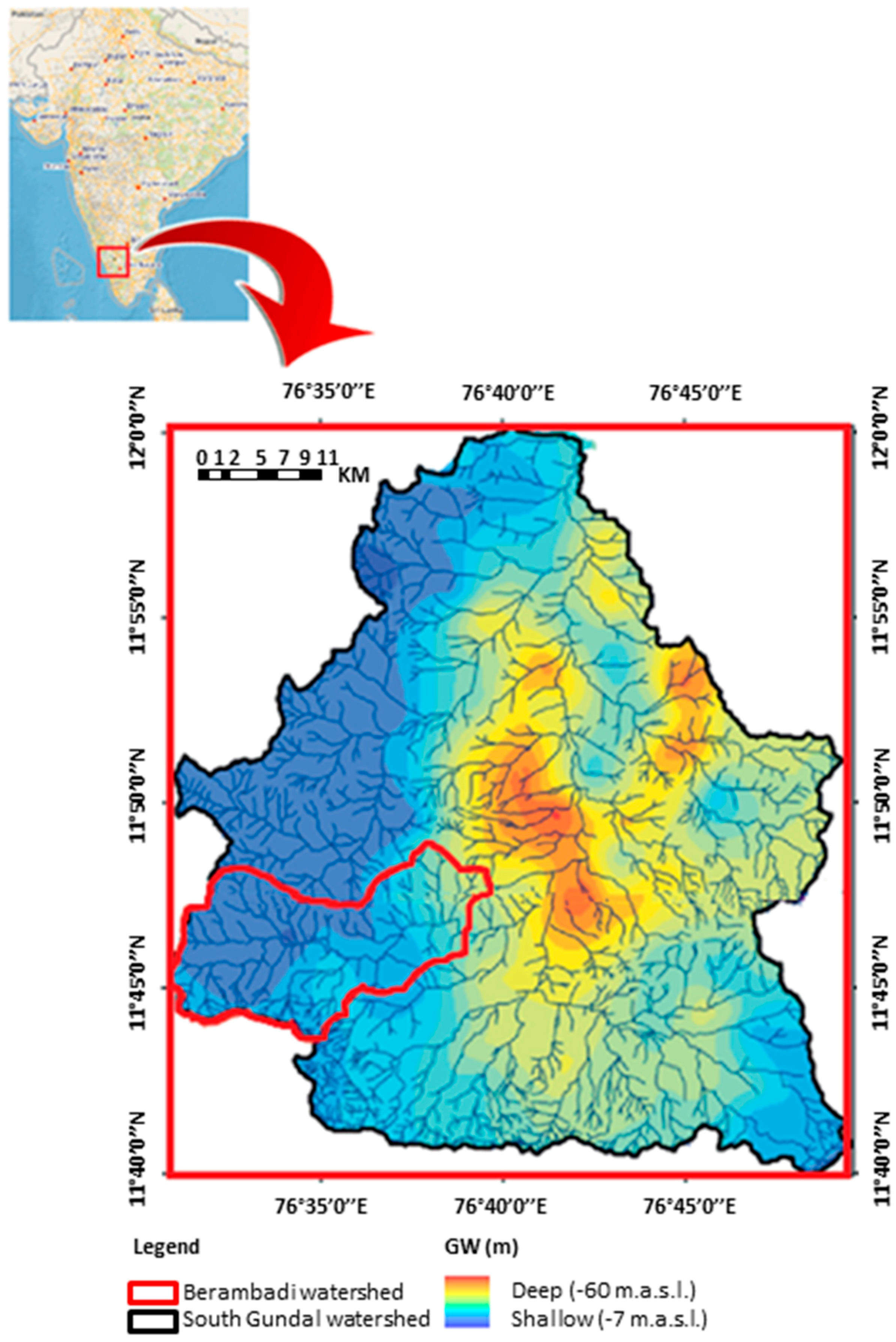
2.1. Case Study: Hydrological and Morphological Description of the Watershed

Berambadi (11°43’00” to 11°48’00” N, 76°31’00” to 76°40’00” E) is an 84 km2 watershed located in southwestern India. It belongs to the South Gundal basin, 816 km2, part of the Kabini River basin (approximately 7000 km2, southwestern Karnataka state), which is a tributary of the Kaveri River basin (Figure 1). Biophysical variables have been intensively monitored since 2009 in the Berambadi watershed, under the Environmental Research Observatory ORE BVET [22] and the AMBHAS observatory [23,24].
Due to the rain shadow of the Western Ghats during the southwestern monsoon rains, the Kabini basin exhibits a steep rainfall gradient, from a humid zone in the west with more than 5000 mm of rain per year to a semi-arid zone in the east with less than 700 mm of rain per year. Since the Berambadi watershed is located in the eastern Kabini basin, its climate is tropical sub-humid (aridity index P/PET of 0.7), with rainfall of 800 mm/year and PET of 1100 mm per year, on average [23]. A moderate east-west rainfall gradient is observed at the watershed scale, with approximately 900 mm rainfall per year upstream (west) and less than 700 mm rainfall per year downstream (east). Three seasons regulate the cropping systems: (1) kharif (June to September), which is the southwestern monsoon season, when almost all plots are cultivated and are either exclusively rainfed or have supplemental irrigation; (2) rabi (October to January), the northeasten monsoon or winter season, when most of the plots where irrigation is possible are cultivated; and (3) summer (February to May), the hot and dry season, when only few irrigated plots are cultivated.
Black soil (Vertisols and Vertic intergrades), red soil (Ferrasols and Chromic Lusivols) and rocky/weathered soil are the main soil types in the area and represent the granitic/gnessic lithology found in southern India [25]. The hard-rock aquifer is composed of fissured granite underlain by a 5–20 m layer of weathered material. Groundwater transmissivity and borewell yields decrease with groundwater table depth [26]. As a consequence, continuous pumping causing groundwater table drawdown leads to a disproportionate decrease of the amount of groundwater available for irrigation [27,28]. This positive feedback loop makes predefined land-use scenarios unrealistic, since farmers need to adapt their actions continually according to groundwater availability [20].
Water table levels display a pattern that is atypical in hydrology: valley regions have deeper groundwater table levels than topographically higher zones. Thus, an unusual groundwater level gradient is observed; with a shallow groundwater table upstream and deep groundwater table downstream (Figure 1). This pattern is the result of intensive groundwater pumping since the early 1990s in villages located in the valley (where soils are more fertile) [19]. The low cost of pumping water and subsidies for irrigation equipment encouraged farmers to drill more borewells [29]. This dramatic change is closely linked to the spatial distribution of soil types and groundwater availability, as well as farming practices, access to the market, knowledge, new agricultural and know-hows, and government aid [19].
An increasing number of farmers report borewell failures for two main reasons: borewells have run dry after excessive pumping, or no water was found in newly drilled borewells [30]. The decrease in groundwater table level disconnected groundwater table from river beds, turning main permanent rivers into ephemeral streams, which has occurred to other rivers in the region [31]. Wells have recently been drilled in upland areas, where groundwater irrigation is increasing.

2.2. Survey Design and Sampling

The farmland ownership register (Bhoomi) of Karnataka lists farmers and land ownership for each village in Karnataka. The Berambadi watershed contains 5461 farm households distributed in 12 villages. To identify how many and which farms to survey in this agrarian community, we used purposive stratified proportional sampling. This sampling procedure is used to estimate distribution parameters for a heterogeneous population [32,33]. The main advantage of this sampling approach is a better representation of the population than other probability methods like simple random sampling or systematic sampling [33]. Indeed, with stratified sampling, even the smallest subgroup in the population can be represented while selecting a relatively small sample size [34]. This ensures that every category of the population is represented in the sample. A stratified sample recreates the statistical features of the population on a smaller scale [35]. In stratified proportional sampling, the sample size of each stratum must be proportional to the population size of the stratum meaning that each stratum has the same sampling fraction. The size of the sample selected from each stratum per village was proportional to the relative size of that stratum in the farmer population. As such, the sampling procedure is self-weighting and an equal-probability-of-selection method. The same sampling proportion was applied to each stratum, giving each element in the population an equal chance of selection. In our farmer population, we stratified the farmers based on the land ownership of farmers. That is, farmers were considered as marginal, small, medium or large owners (e.g., variable totalHHSize in Table 1).
The samples were purposefully selected to represent the caste diversity in the region. In total, 684 farm households, which represent 12.5% of farms on the watershed, were interviewed from September 2014 to March 2015. The survey consisted of a face-to-face interview lasting 2–3 h. The survey was divided into three parts. The first part focused on household characteristics, farm structure, assets, partnerships, and farm objectives. In the second part, we asked farmers about their performances and practices over the past two years (2013–2014). The absence of a record of past practices made it difficult to obtain data on past cropping systems and farm activities that occurred more than two years ago. Incomes from selling crops were available for 2013. Concerning farm expenditure, farmers were comfortable in providing information for the most recent cropping season—kharif 2014. In the last part, in-depth questions were asked about irrigation, borewells, and rainfall. Since no yearly records were kept by farmers, information about historical management went no further than the past two years.

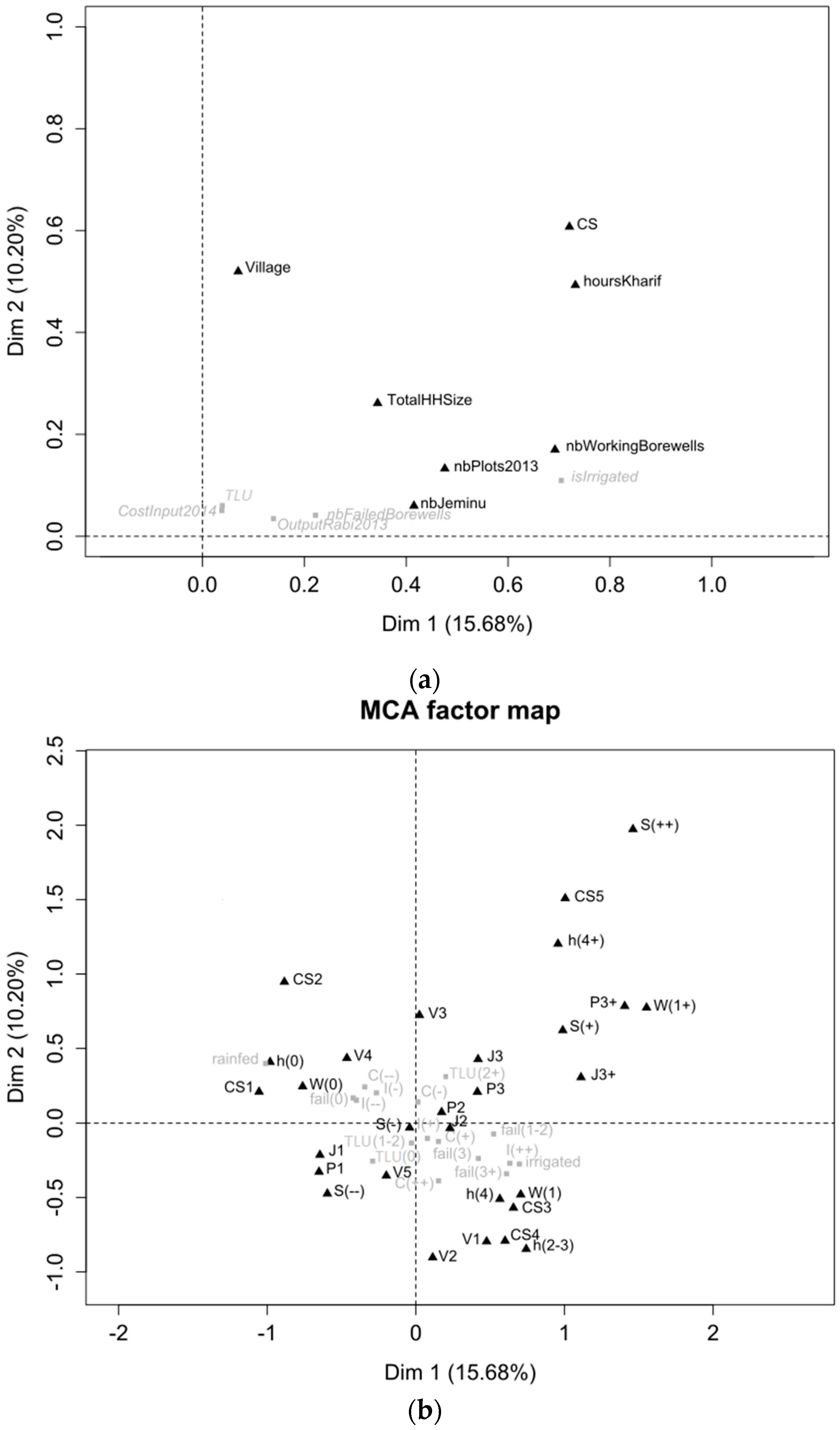
2.3. Analysis Method

First, we identified variability in farm characteristics and farming practices on the watershed, based on farmer surveys. Four dimensions were analyzed: (1) farm structure; (2) the cropping system and farm practices; (3) water management for irrigation; and (4) economic performances of the farm. To examine the variability and spatial pattern of each dimension on the watershed, we used the village as the spatialized indicator. To determine the overall significance of differences among villages, the means of the qualitative variables were compared by an analysis of variance (ANOVA) permutation test whereas the independence between qualitative variables were tested by chi-square tests. We considered the differences among villages significant at the 95% level. Analyses were performed with the R language and environment for statistical computing [36].
Second, we used the results of the previous analysis to establish a typology of farms based on the farm characteristics and farming practices describing some variability on the watershed. We performed a two-step statistical analysis. The first step used the nominal categorical data technique of Multiple Correspondence Analysis (MCA). MCA is an extension of correspondence analysis for more than two variables. Compared to principal component analysis, MCA allows the use of both quantitative and qualitative variables. The non-correlated quantitative variables were converted into qualitative variables with associated modalities (classes) and then used for MCA analysis. [37,38]. However, transforming quantitative variables into qualitative ones may lead to a loss of some of its properties as well as the measurement precision. The principle of MCA is to define factors representing an optimized quantitative summary of the relationships between variables [39]. Compared to other statistical methods, MCA has some interesting advantages. The MCA procedure does not require any preconditions on variables (such as multivariate normality or linearity) and it offers statistical results that can be seen both analytically and visually. The MCA is a preprocessing step for the classification or typology purposes. It provides qualitative values derived from categorical variables needed in deterministic cluster analysis [40]. The principal components of the MCA were then used as input variables in an Agglomerative Hierarchical Clustering (AHC) algorithm. It starts with as many clusters as farms and progressively sorts the farm by building up a tree from successive merges of the two nearest clusters. The AHC procedure is often represented by a two dimensional diagram (dendrogram) which illustrates the classification obtained at each successive stage of the analysis. This method successively groups the closest farms into clusters, which then are grouped into larger clusters of higher rank (farm types) by partitioning farms based on their factorial coordinates using the Ward’s minimum-variance aggregation method criterion for minimizing intra-cluster variance and maximizing variance between clusters [41,42].
The farm types can then be described by the quantitative variables with the coefficient of determination and the p-value of the F-test in a one-way ANOVA (assuming homoscedasticity).

3. Variability and Spatialization of Farm Characteristics and Practices

3.1. Farm Structure

3.1.1. Household Characteristics

At the Berambadi watershed scale, three gram Panchayats (The Panchayat is the system of local self-government. The basic unit of the Panchayats in India is known as the “gram Panchayat” [43], namely the village council that is elected in the popular voting system. The principal functions performed by the gram Panchayats are maintaining roads, wells, schools, burning and burial grounds, sanitation, public health, libraries, reading rooms, community centers, etc.) were identified: (i) Bheemanabeedu gram panchayat for the eastern villages; (ii) Kannagala gram panchayat for the central villages and (iii) Berambadi gram panchayat for the western villages. The eastern portion of the watershed is statistically dominated by the Upparas sub-caste, and the central and western portions consist mainly of the Schedule Caste and Lingayat (Figure 2).
The average household in the watershed is composed of four adults (2 men and 2 women) and one elder person (>60 years old). Overall, 86% of households investigated are headed by a man of 58 years of age, on average, who is usually illiterate (61% of heads-of-household are illiterate). Men usually work full-time on the farm, while women work part-time on the farm and perform the domestic work. Agricultural labor is a secondary occupation for 16% of the interviewed population. Few people migrate to work in other places during rabi season (people migrate in only 4% of households). Households in the Berambadi gram panchayat are statistically smaller, with three adult members and one elderly person. A larger percentage of farmers are better educated in the Kannegala gram panchayat, and over 50% attended at least pre-primary school (vs. 20% in the rest of the watershed) (Figure 2).

3.1.2. Land Holding

Average farm size in the watershed is 1.2 hectares and varies from 0.01 to 9.3 hectares. Most farms are small (48% have 0.8–2 hectares) or marginal (32% have <0.8 hectares). Only 17% of farms have more than 2 hectares, while 3% have more than 4 hectares. Farmers own their farmland. A field with adjacent agricultural plots cultivated by the same farmer is called a “jeminu”. A farm can comprise several “jeminus”, which may or may not be located nearby each other; they can even be located in different villages. Overall, 45% of farmers have only one jeminu, while 26% have 2, 13% have 3 and 16% have more than 3. The entire jeminu can be dedicated to one crop each season (54%) or divided into several crop plots (31% with 2 crop plots, 14% with 3–5 crop plots). On average, a crop plot is 0.4 hectare but varies from 0.01 to 2.4 hectares.
Land holding is variable on the watershed. Statistically, more marginal farms (<0.8 ha) exist in the Beemanabeedu gram panchayat (42%, vs. 23% in the rest of the watershed), where farms are more fragmented (80% of farms in the Beemanabeedu gram panchayat have more than 1 jeminus vs. 55% in the rest of the watershed). Farms in the Berambadi gram panchayat are less diversified: 80% cultivate only one plot with one crop (vs. 60% in the rest of the watershed) (Figure 2).

3.1.3. Livestock and Equipment

Even though livestock production is usually a secondary activity, farmers have animals for traction, milk, meat and breeding. To represent the livestock intensity we built a coefficient of Tropical Livestock Unit (TLU) where cows, oxen, buffalos, and bulls are 1 TLU and sheep and goats equal 0.2 TLU [44]. Farmers have an average of 2 TLU.
The traditional equipment for soil operations is based on animal traction. Motorization recently spread, and plowing with a tractor now commonly supplements the traditional animal work. However, tractors are expensive, and most farmers (94%) prefer to rent from a tractor owner in the village rather than obtaining a loan to buy one. Farmers use oxen, bulls and buffalos along with a plow (96% use a plow and 87% own one). Farmers who own animals for traction usually have only one pair of animals. A pesticide sprayer is the most common equipment used for farming operations in the Berambadi watershed (88% use a sprayer and 61% own one). Seeders, weeders and rotovators are rarely owned or used in the watershed. Seeding, fertilizing, weeding and harvesting are usually performed manually and do not require specific equipment.
Equipment use varies spatially across the watershed. The percentage of farmers owning buffalos is statistically the highest in the Kannegala and Berambadi gram panchayats. Statistically, a pesticide sprayer is owned mainly by farmers in the Beemanabeedu and Berambadi gram panchayats. Livestock ownership varies statistically across the watershed: more than 50% of farmers own at least 2 TLU in the Kannegala and Berambadi gram panchayats, while 20% of farmers own at least TLU in the Beemanabeedu gram panchayat (Figure 2).

3.1.4. Labor

Because many technical operations are manual, farming practices are highly labor-intensive. Only two farmers employ permanent workers; they hire workers on a daily basis or based on crop-operation contracts. Women typically perform sowing, weeding and harvesting, and men typically perform soil preparation, fertilization, pesticide treatment and irrigation. In 2013 and 2014, 40 male workers and 84 female workers were hired on average per hectare for the cropping season. No significant spatial variability was found in labor per hectare across the watershed.

3.2. Farm Practices

3.2.1. Input Use

The amount of input purchased per unit of cultivated area decreases on a northwest-southeast gradient. Villages from the Berambadi gram panchayat have higher expenses for pesticides (3750 Rs/hectare) and chemical fertilizers (6250 Rs/hectare). The percentage of farms that do not use manure is also statistically higher (40%–80%) in villages from the Berambadi gram panchayat, which reinforces dependency on chemical inputs. While the purchase of pesticides strongly decreases along this gradient (reaching only 750 Rs/hectare in the Beemanabeedu gram panchayat), the decrease in the purchase of chemical fertilizer is lower (from 6250 to 4500 Rs/hectare) (Figure 2).

3.2.2. Crop Yield Performances

Crop yields vary greatly among fields. However, high-input villages from Berambadi gram panchayat and low-input villages from Beemanabeedu gram panchayat have particularly low yields (<2.5 t/hectare, on average, for rainfed sorghum, or irrigated maize). Villages in the Kannegala gram panchayat have statistically better results, (>2.5 t/hectare, on average and up to 10 t/hectare for for the same crops) (Figure 2). In villages from the Kannegala and Berambadi gram panchayats, more than 30% and 35% of farming areas are grown for subsistence whereas only 5% of the farming areas of villages from the Beemanabeedu gram panchayat are grown for subsistence.

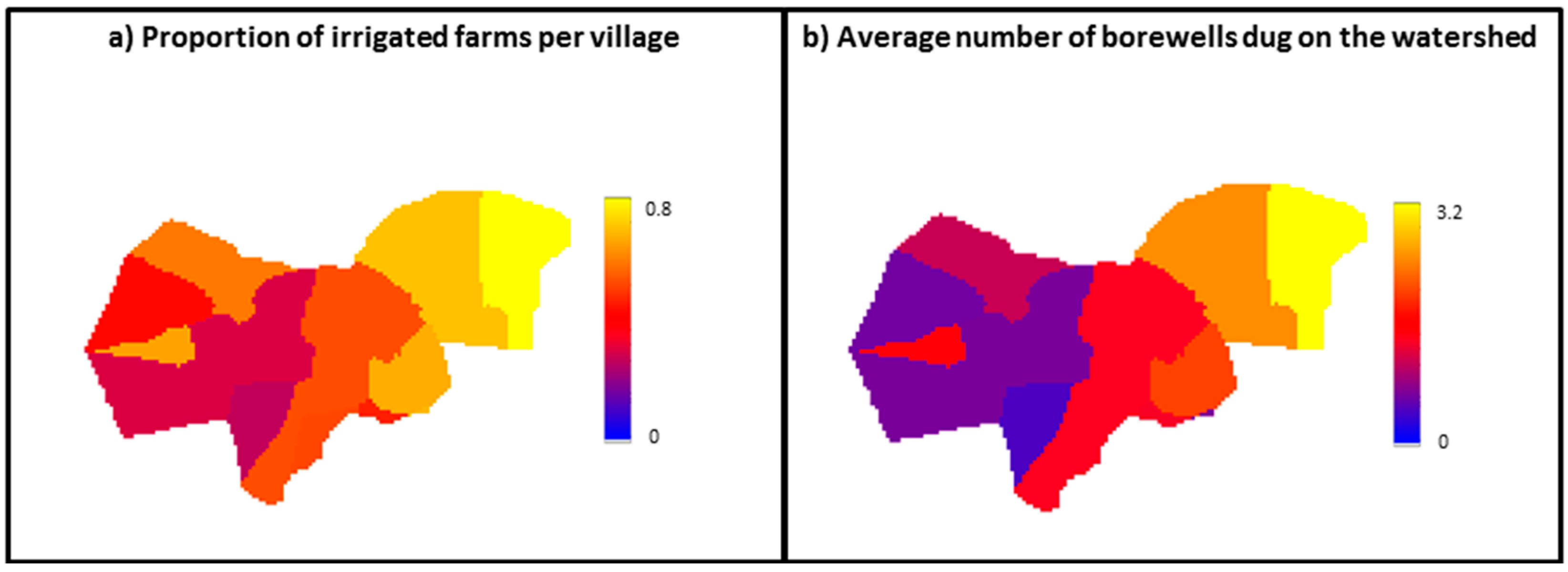
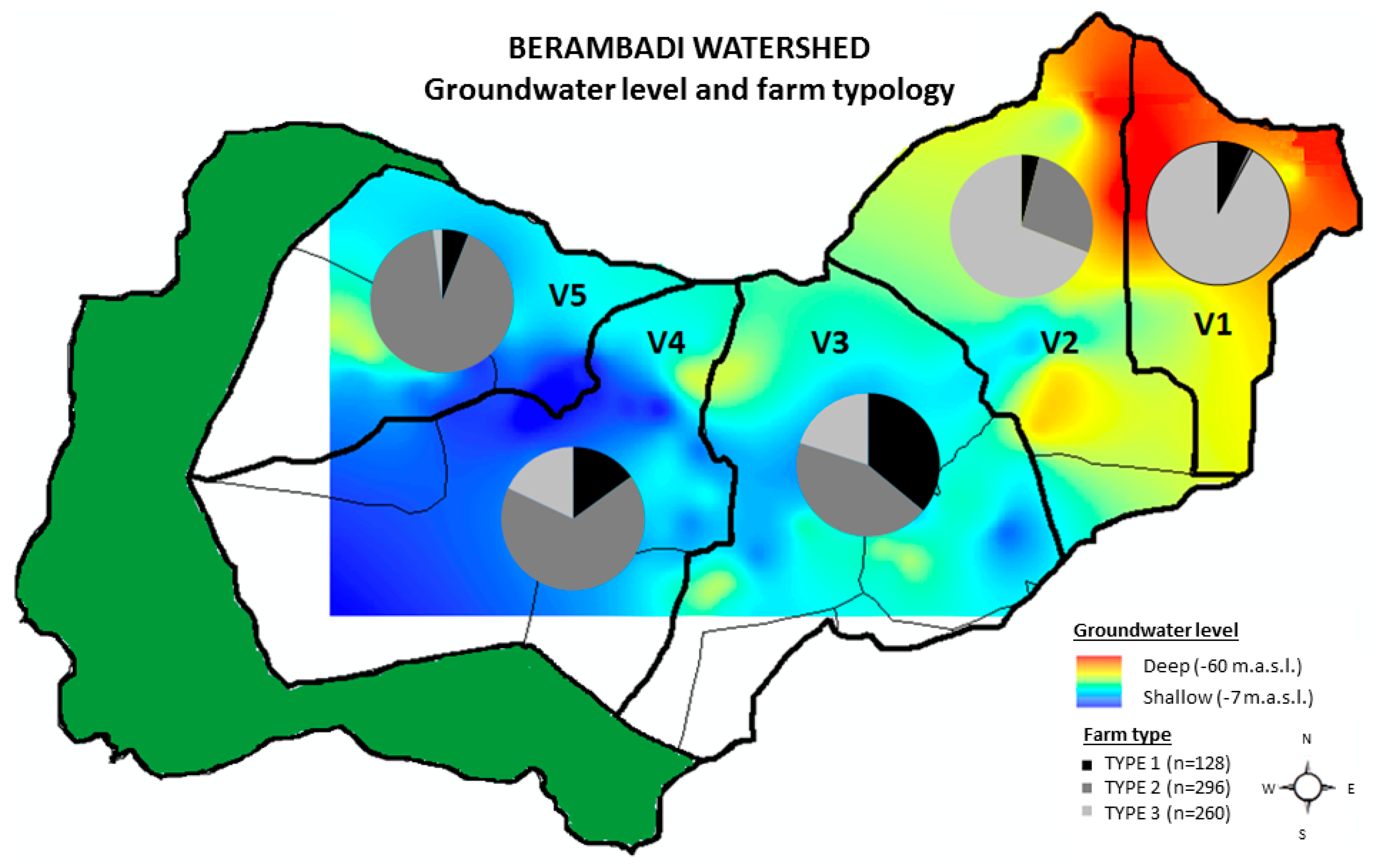
3.3. Water Management for Irrigation

3.3.1. Access to Irrigation
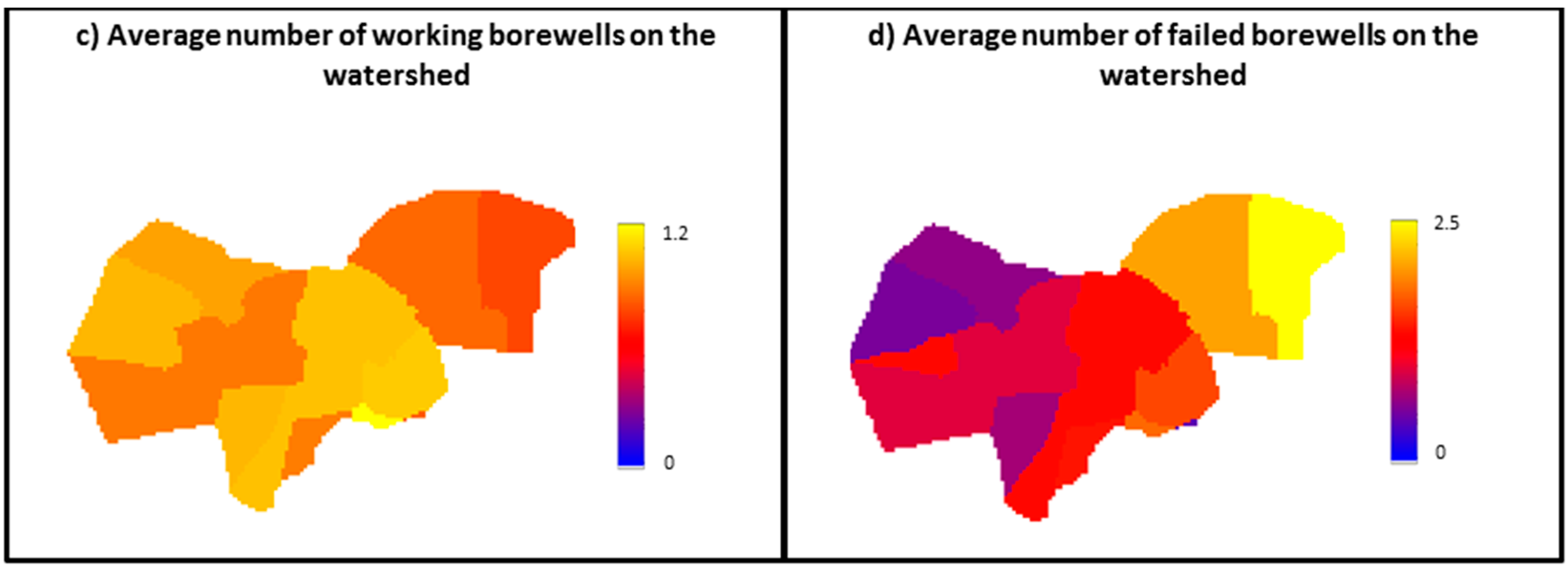
Overall, 59% of farms have access to irrigation. Irrigated farms have on average more jeminus than non-irrigated farms: 32% of irrigated farms vs. 63% of non-irrigated farms have only one jeminu. Farms with only one jeminu are mainly rainfed (58%), while 73% of farms with more than one jeminu are irrigated. For 63% of irrigated farms, all the jeminus have access to irrigation. All the surveyed farms with access to irrigation directly use groundwater on their fields or temporarily store it in individual farm ponds. We observed only a few cases of exchange or sale of water between farmers. Statistically, more irrigated farms exist in the Beemanabeedu gram panchayat, where they represent approximately 80% of the farms.

3.3.2. Borewells

The first borewells in the watershed were drilled in the 1970s, and borewell drilling has increased dramatically since the mid-1990s. In our sample, 31 borewells were drilled before 1995, and 470 borewells were drilled after 1995. In the 1970s and 1980s, most borewells were drilled in the Beemanabeedu and Kannegala gram panchayats, while in the Berambadi gram panchayat well drilling occurred mainly in the 2000s. In addition to the increasing number of borewells, technology has allowed drilling deeper wells. The maximum depth of wells drilled before 1995 was 150 m, while 15% of the borewells drilled from 1995 to 2010 were deeper than 150 m. Among the 214 borewells drilled after 2010, 25% were deeper than 150 m, with the deepest reaching 250 m.
From the survey sample of 1192 borewells, 33% were working at the time of the survey, while 58% had failed (i.e., produced no water), and 9% had been temporarily stopped since 2013. No relation was found between the depth of a borewell and whether it worked, had been stopped or had failed. There are as many farms with at least one no working borewell as farms on which all borewells work (115 and 105 farms, respectively, of the 245 farms that had drilled at least one borewell). Overall, 49 farms (7%) that attempted to drill borewells never got groundwater for irrigation.
Figure 3 summarizes the spatial distribution of irrigated farms and their borewell characteristics within the watershed. Each farm has drilled approximately three borewells in the Beemanabeedu gram panchayat vs. less than one in the Berambadi gram panchayat, which is consistent with irrigated farms being located predominantly in the Beemanabeedu gram panchayat villages. However, borewell failure has occurred predominantly in the Beemanabeedu gram panchayat villages (more than 65% of borewells drilled in the Beemanabeedu gram panchayat villages have failed, vs. 53% in the Kannegala gram panchayat villages, and 35% in Berambadi gram panchayat villages), which results in a relatively uniform number of working borewells per farm within the watershed.

3.3.3. Pumps and Access to Electricity

Farmers use electric pumps, mostly of 7.5 horse power (HP). Farmers who need electricity, i.e., those with at least one working borewell, have approximately 3–4 h of electricity per day during kharif and 2–3 h/day during rabi, with on average 2–4 power outages per day. The duration of electricity supply during kharif is statistically higher in the Kannegala gram panchayat villages, where 69% of farms have more than 4 h of power per day. Electricity is usually available less than 4 h/day in the rest of the watershed (Figure 2).

3.3.4. Farm Ponds

Farm ponds are shallow ponds in which farmers store pumped water for distribution throughout the day, especially during power outages at critical times. It takes 2–9 h to fill a farm pond. Approximately 290 individual farm ponds exist on the surveyed farms, and only 36% of farms have one. No relationship was found between farm pond ownership and location on the watershed.

3.3.5. Irrigation Methods

Among irrigated farms, 81% use only one irrigation method. Furrow irrigation is by far the most common method (75% of irrigated farms), mainly as the only irrigation method (58%), and more rarely is used in combination with a sprinkler or drip (17%). Among alternative methods of irrigation, sprinklers (17% of the jeminus) are used more often than drip irrigation (3% of the jeminus) or flood irrigation (2% of the jeminus). Sprinkler irrigation statistically occurs more in the Beemanabeedu gram panchayat villages (37%–78% of jeminus, depending on the village), while the Berambadi gram panchayat villages almost exclusively used furrow irrigation (94% of jeminus) (Figure 2).

3.4. Economic Performances of the Farm

3.4.1. Investment in Farm Structure

Considering investments in equipment and livestock, farmers owned an average of 4500 Rs/hectare of equipment 18,670 Rs/TLU of livestock at the time of the survey. On average in 2013–2014, farmers hire 22,100 Rs/hectare of labor each cropping season, with male wages fixed at 250 Rs/day and female labor at 150 Rs/day. The only clear statistical difference in investment in farm structure is the livestock investment, which is slightly higher in the Kannegala and Berambadi gram panchayat villages than in the Beemanabeedu gram panchayat villages due to greater use of animal traction for cultivation.

3.4.2. Cropping Systems’ Products and Expenses

Fertilizers and pesticides cost approximately 12,700 Rs/hectare during kharif 2014. Overall, 99% of farmers buy some or all of their inputs from retailers, 8% purchase some of their inputs from a cooperative and 64% obtain them from government suppliers. A higher percentage of farmers obtain inputs from a cooperative in the Berambadi gram panchayat villages (>25%), whereas a lower percentage do so in the Kannegala and Beemanabeedu gram panchayat villages. Selling crops during kharif yield an average of 39,900 Rs/hectare in 2013. For kharif, no difference is observed across the watershed. Only 74% and 9% of farmers sell cash crops during rabi and summer, respectively. Rabi crops earn approximately 9630 Rs/hectare, while summer crops earn approximately 25,750 Rs/hectare in 2013. A statistically higher percentage of farmers grow cash crops during rabi in the Beemanabeedu gram panchayat villages, where more than 50% earn more than 12,500 Rs/hectare during rabi, vs. less than 30% in the Berambadi gram panchayat villages.

3.4.3. Investment in Irrigation

Investment in a borewell is based on its depth. The deeper the borewell is, the more it will cost to drill. However, borewell drilling has a fixed cost per meter (approximately 410 Rs), regardless of the depth at which drilling begins. Farmers typically maintain a borewell five years after drilling it (62% of borewells, while 24% are maintained 5–10 years after drilling). Maintenance costs approximately 6000 Rs per borewell over the borewell life. Investment in pumps varies. The main investment is 7.5 HP pumps (61%), which at approximately 28,000 Rs, cost 3000–7000 Rs more than pumps with less HP. Investments linked to water management do not vary across the watershed.

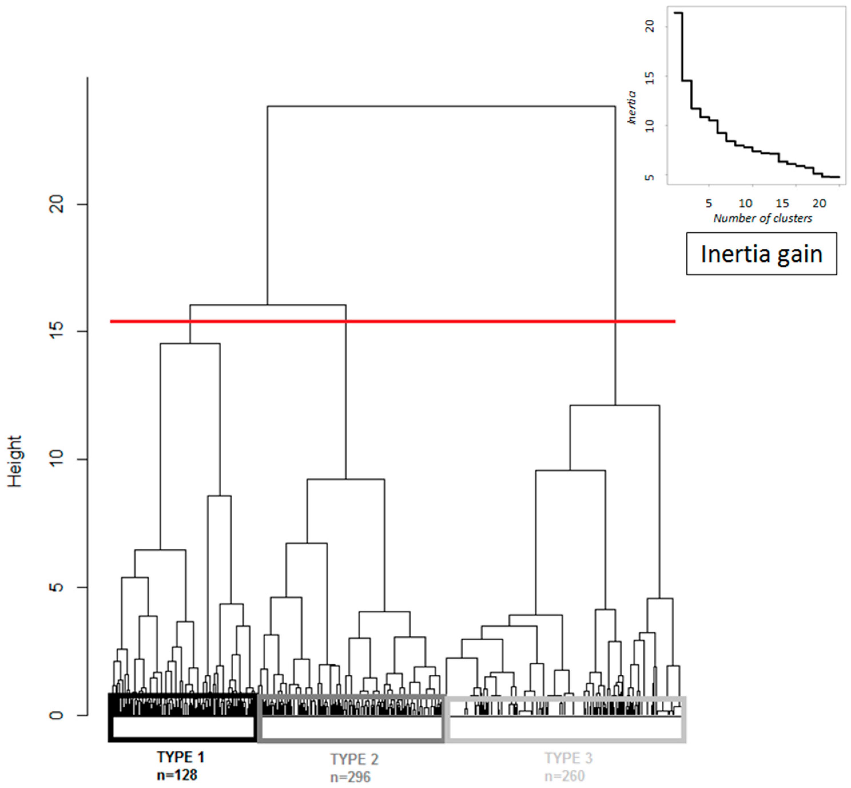
4. Typology of Farms in the Berambadi Watershed

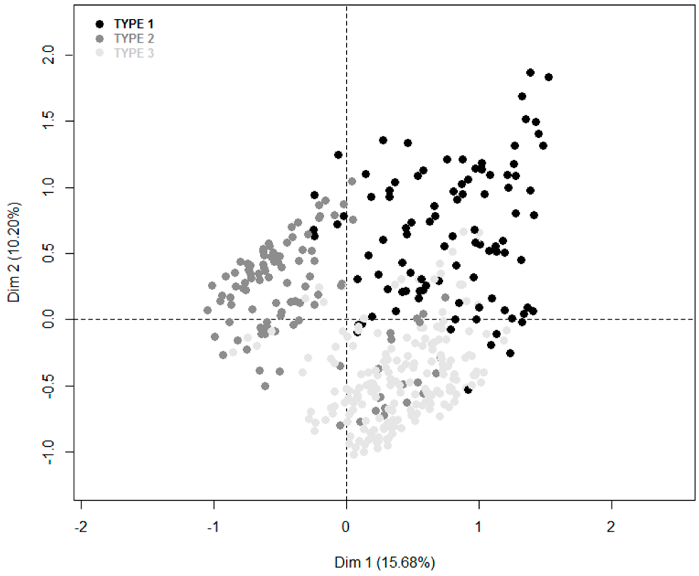
4.1. Characteristics of Farm Typology

The survey identified nearly 50 qualitative and quantitative variables on the farming context, farm performance and farming practices. Following the previous analysis and after checking for correlation and homogeneity among the households, we tested 12 variables in the MCA (Table 1). The variables that had less weight on the four first axes were used as complementary variables. Variables that describe the farming context included those related to the spatial location of the farm and resources for the farmland, irrigation and animals. Farm location is described by the village. The 12 villages in the watershed were combined into five ‘big’ villages (V1, V2, V3, V4, V5) based on similarities in their groundwater tables. The land-resource variables (3) are farm size, number of jeminus and number of plots. The irrigation-resource variables (4) are access to irrigation, the number of failed and working borewells and hours of electricity available per day for pumping. The animal resource is summarized into the class of livestock variable. Variables that describe the farm performances include those related to production costs (input costs spent per hectare in kharif 2014) and incomes (rabi incomes per hectare in 2013). Farming practices are included in the cropping system variable, which distinguishes cropping systems by irrigation practice and crop purpose (cash crop or subsistence).
The first two components of the MCA explain 25.9% of the total variability in individuals (Figure 4). The third and fourth components explain 8.1% and 7.1% of the total variability in individuals, respectively. The first axis discriminates (1) rainfed farms that grow rainfed crops without access to irrigation water and (2) irrigated farms that grow mixed crops based on irrigation water from borewells and access to electricity (Figure 4). The second axis discriminates (1) large farms (S(+)) with several jeminus (J3+) and several plots that use water from borewells located in the center of the watershed (V3 and V4), where electricity is more available (hours(4+)) and that grow irrigated and rainfed crops for cash and subsistence purposes (CS5 and CS2) from (2) smaller farms (S(-) and S(--)) located in the eastern and western portions of the watershed (V1, V2 and V5) that grow crops on one or two plots (J1 and J2) as a cash crop (CS4 and CS3) and have less available electricity (hours(2–3) and hours(4)).
The MCA allowed us to reduce the number of dimensions in the qualitative data by selecting the first 12 components of the MCA, which collectively explained 79.1% of the total variation. The first 12 principal components in an AHC algorithm were then used as input variables in an Agglomerative Hierarchical Clustering (AHC) algorithm. The choice of the number of clusters for the partition was made relative to the general shape of the tree, the gain of inertia between the clusters when adding a cluster and the interpretability of the clusters. To identify the number of farm types (clusters) we identified the maximum jump in between-cluster inertia [45] (Figure 5). We obtained a typology with three farm types (Figure 5). Three groups are clearly distinguishable on the projection of individuals in the plane of the first complete MCA (Figure 6).

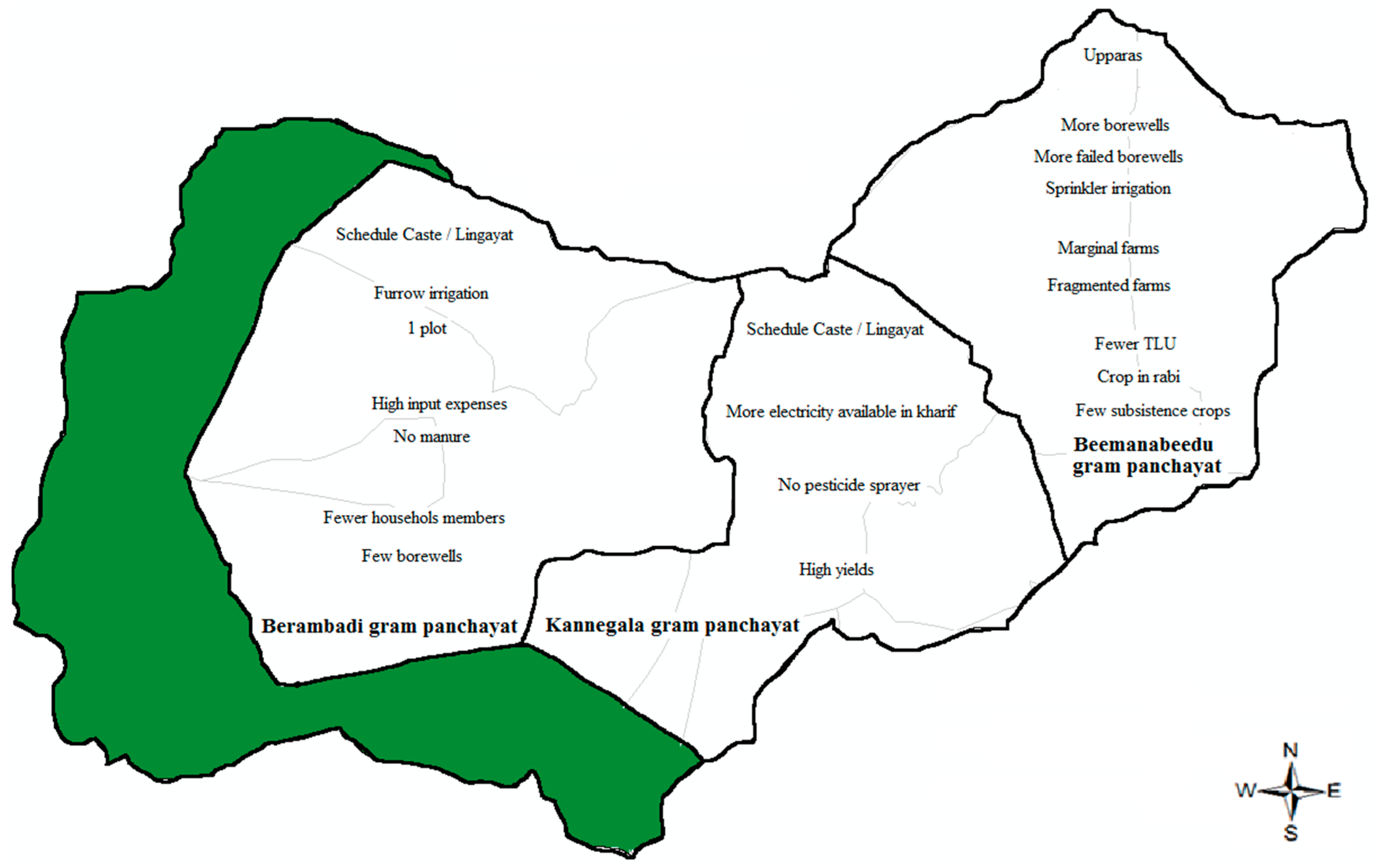
4.2. Characteristics of the Farm Types

Characteristics and homogeneity of the three farm types identified based on the survey data are presented in Table 2.

4.2.1. Farm Type 1: Large Diversified and Productivist Farms

Type 1 farms are located mainly in the center of the watershed (73% of type 1 farms are in V3, where 36% of farms are type 1) (Figure 7 and Table 2). This type represents all large farms in the sample and some medium farms (39% of type 1 farms are medium) with the highest amount of electricity available for pumping (56% of type 1 farms have >4 h/day). Overall, 56% of type 1 farms have more than 2 hectares of land. These large farms are often composed of several jeminus where farmers can easily cultivate several plots. Nearly all type 1 farms have the same water access. Overall, 97% of these farms are irrigated from one or more borewells. However, access to groundwater for irrigation is risky and costly; 64% of these farms also experienced borewell. Overall, 88% of these farms graze livestock to provide animal traction and manure. Input costs and income from selling cash crops are diversified in this farm type. Farming practices are diversified, with cropping systems that mix irrigated and rainfed crops grown as cash crops or for subsistence (53% in CS5) or as cash crops only (19% in CS3 and CS4).

4.2.2. Farm Type 2: Small and Marginal Rainfed Farms

Type 2 includes marginal and small rainfed farms located in the central (39% of type 2 farms are in V3) and western portions of the watershed (45% of type 2 farms are in V4 and V5) (Figure 7 and Table 2). More than 90% of these farms have less than 2 hectares on one jeminu and operate on 1–2 plots. They have no access to irrigation, and few have ever attempted to drill a borewell. Due to the absence of irrigation, it is difficult to grow crops during rabi (62% earned < 37,000 Rs/hectare in 2013). These small farms have the lowest farming expenditures (64% invested < 7400 Rs/hectare in fertilizers and pesticides during kharif in 2014). While 65% grow only cash crops, the other 35% grow also subsistence crops to cover household needs.

4.2.3. Farm Type 3: Small Irrigable Marketing Farms

Type 3 consists of small irrigated farms located in the eastern portion of the watershed (72% are in V1 and V2) (Figure 7 and Table 2). Overall, 85% of type 3 farms have less than 2 hectares on one jeminu and operate on 1–2 plots. Farmers have at least one borewell, and 67% have experienced a failed borewell. Electricity for pumping is less available in this portion of the watershed than in the center (type 1). In general, farmers have medium to large expenses balanced by medium to large incomes from selling crops. Cropping systems are diversified by mixing irrigated and rainfed crops, but all production is reserved for cash crops (91% of farms in CS3 and CS4).

5. Discussion

Irrigation technology developed after 1995 greatly influenced groundwater table depletion in the Berambadi watershed. In addition to this technological development, expected future change in regional climate might lead to higher evapotranspiration which could result in decrease of groundwater recharge. To preserve the depth of the groundwater table and minimize its depletion due to agricultural practices, a variety of policy interventions are possible for promoting water-management practices that reduce pumping and groundwater depletion, including changing the conditions of electricity supply for irrigation or promoting water-efficient crops or irrigation techniques. However, to be efficient and accepted by farmers they should be adapted to farm characteristics and objectives.
Farm typologies are critical for representing while also simplifying the diversity of farms in a large area. Specifically, farm typologies are critical to effectively represent the heterogeneity of farmers’ objectives and socio-eco-agronomic conditions relative to their decision-making processes regarding farm management. The sample selection and statistical analysis used to generate the typology may influence the latter’s quality. Access to the Karnataka land-ownership register was critical for identifying a sample that statistically represented the population of the watershed based on farmers’ land ownership. The survey process was in the local language, which made it difficult to understand specific agronomic terms and concepts. The absence of a record of past practices made it difficult to obtain data on past cropping systems and farm activities that occurred more than two years ago. The data obtained were based mainly on farmers’ reports. Except for village affiliation, no other spatial indicator was collected in the survey. An important issue in the field was obtaining the exact location of a farm within a village.
The combination of multivariate statistical techniques and cluster analysis is widely used in characterization studies and farm-typology studies (e.g., [33,40,46,47], Goswami et al [46] combined principal component analysis with a hierarchical method and a K-means clustering method to develop a typology of farms and economic characteristics in India. Laoubi et al. [33] used MCA and AHC to develop a typology of irrigated farms in Algeria. Milán et al. [47] used MCA and cluster analysis to develop a typology of beef-cattle farms in Spain. Kristensen et al. [40] developed a typology of farms, farmer characteristics and landscape changes in Denmark by combining MCA and AHC.
The Berambadi watershed is a small region where farms had certain characteristics that were relatively similar, unlike other studies conducted at state or district levels. For instance, household composition and organization (i.e., family size, family members’ main occupation, and migration) were similar in the Berambadi watershed. Goswami et al [46] conducted a study at the district level in the South 24 Parganas district in West Bengal, and Senthilkumar et al. [48] conducted a study at the state level in Tamil Nadu (the neighboring state to the south of Karnataka). Both studies showed that family size and off-farm income were heterogeneous in larger regions. Seasonal migration of rural labor is a common problem in rural India [49,50,51] but was not observed in our survey. However, farm ownership is an inheritance of the land reform in 1947, which redistributed land to poor farmers by restricting the size of landed property [52].
The development of borewells observed in the Berambadi watershed since the 1970s also occurred in other parts of India, especially in other hard-rock aquifer areas such as Madhya Pradesh, were the number of borewells increased by nearly eleven times from 1986 to 2001 [53]. This trend generated a high density of borewells that caused them to interfere with each other [18]. Borewell interference occurs when a borewell’s area of influence comes into contact with or overlaps that of a neighboring borewell [18,53]. Borewell interference may be one reason for the high percentage of borewell failures. Borewell failure is often due to failure in identifying the exact water-bearing zones or aquifers, which is common in hard-rock regions in India [53,54]. Results showed that technological developments increased borewell depth over the past 10 years in the Berambadi watershed. However, a recent study on hard-rock aquifers in Karnataka demonstrated that nearly 70% of all fractures occur within a depth of 100 m, and the probability of encountering fractures decreases considerably below 100 m [55]. Aubriot [18] indicated that farmers’ willingness to drill deeper may be linked to social and prestige-related aspects.
The spatialization of the typology was based on the village which is recognized as an important criterion for spatialization to consider for instance the social structure (see panchayat). Other criteria may be interesting for spatialization such as the distances to main roads, the soil properties and the groundwater level at the farm location to discuss the access to markets and crop outlets as well as constraints to crop choices and farming practices. Farm-type locations in the watershed follow an east-west gradient, with more irrigated farms in the east and more rainfed farms in the west (Figure 7). This farm-type distribution is linked to the trend in investing in irrigation since the 1990s which caused the unusual inverse gradient of the groundwater table [13,14].
The typology presented here was based on farming context, farm performances and farming practices. We identified three types of farms: (1) large diversified and productivist farms located mainly in the center of the watershed; (2) small and marginal rainfed farms located in the central and western portions of the watershed; and (3) small irrigable marketing farms located in the eastern portion. This typology is similar to the one generated in Tamil Nadu [46,56] where a first type, including the wealthiest farms with large irrigated land holdings (average = 6 hectares), were distinguished from a second type, including medium wealth with an average land holding of 3 hectares, and from two other types of farms considerably poorer and marginal at meeting their family food requirements based on rainfed crops grown during the monsoon season.
This typology makes it possible to simplify and represent farm diversity across the watershed. The study’s results are specific to its purpose and study area. The farm types identified cannot necessarily be extrapolated to a larger context outside the Berambadi watershed. For instance, the farm typology developed in West Bengal [46] differs from ours mainly because of the diversity of farming systems identified there. While we identified five cropping systems based on access to irrigation (irrigated and/or rainfed cropping systems) and crop orientation (cash and/or subsistence cropping systems), they distinguished four farming systems based on the sources of farmers’ maximum gross income. These included rice, vegetables, fish and off-farm based farming systems. However, the two-step method combining MCA and AHC is subject to generalization for even larger regions [33,40,46,47].
This study predicts two scenarios for the watershed: (1) farmers, especially on small, irrigated marketing farms and large productivist irrigated farms, may continue to maximize profits by producing high water-demanding crops and cash crops; and (2) irrigation technology may continue to spread toward the western portion of the watershed and convert small rainfed farms into small irrigable marketing farms. Simulation models may help determining whether these scenarios may be sustainable in terms of groundwater depletion and farmers’ incomes.

6. Conclusions

The typology presented here should enable policy makers to better assess the potential influence of agricultural and water-management policies on farmers’ livelihoods and the groundwater table. The typology can be used in simulation models to predict impacts of climate change, specifically higher evapotranspiration, on farming practices and the groundwater level. Such simulation models are useful to test policies aiming to slow groundwater-table depletion and limit income risks due to crop failure. For example, simulation models could explore policies to maintain small rainfed farms (e.g., subsidizing rainfed crops, especially subsistence crops such as pulses) or policies to encourage farmers to adopt better water management in cropping systems, (e.g., decreasing the area of crops that consume large amounts of water, such as banana, sugar cane and turmeric, or modifying electricity availability or subsidizing drip irrigation or less water consuming crops or varieties).

Acknowledgments

This study was part the multidisciplinary Indo-French research project AICHA (Adaptation of Irrigated Agriculture to Climate Change 4700-W1) funded by the Indo-French Centre for the Promotion of Advanced Research (CEFIPRA), the INRA flagship program on Adaptation to Climate Change of Agriculture and Forest (ACCAF), the Doctoral School of the University of Toulouse (EDT) and ORE BVET. We are grateful to all the experts, farmers, and trainees who helped implement the method. We are also very grateful for the help and hard work of the field team. Particular thoughts go to Jarayma and his family, to whom we convey my sincere condolences.

Author Contributions

All co-authors participated in conceiving and designing the study. Marion Robert, Shrinivas Badiger, Jacques-Eric Bergez, Alban Thomas, Delphine Leenhardt and Magali Willaume conceived and designed the farmer survey. Shrinivas Badiger coordinated the implementation of the farmer survey and Marion Robert participated to the farmer survey. Marion Robert, Alban Thomas, Delphine Leenhardt, Jacques-Eric Bergez and Magali Willaume carried out the data analyses. Muddu Sekhar and Laurent Ruiz conceived and coordinated the biophysical monitoring of the Berambadi watershed and carried out analyses of biophysical data. Marion Robert wrote the first draft of the paper. All co-authors contributed to writing the manuscript.

Conflicts of Interest

The authors declare no conflict of interest.

References

  1. Ragab, R.; Prudhomme, C. SW—Soil and Water. Biosyst. Eng. 2002, 81, 3–34. [Google Scholar] [CrossRef]
  2. Fishman, R.; Devineni, N.; Raman, S. Can improved agricultural water use efficiency save India’s groundwater? Environ. Res. Lett. 2015, 10, 84022. [Google Scholar] [CrossRef]
  3. Graveline, N. Economic calibrated models for water allocation in agricultural production: A review. Environ. Model. Softw. 2016, 81, 12–25. [Google Scholar] [CrossRef]
  4. Valverde, P.; de Carvalho, M.; Serralheiro, R.; Maia, R.; Ramos, V.; Oliveira, B. Climate change impacts on rainfed agriculture in the Guadiana river basin (Portugal). Agric. Water Manag. 2015, 150, 35–45. [Google Scholar] [CrossRef]
  5. Köbrich, C.; Rehman, T.; Khan, M. Typification of farming systems for constructing representative farm models: Two illustrations of the application of multi-variate analyses in Chile and Pakistan. Agric. Syst. 2003, 76, 141–157. [Google Scholar] [CrossRef]
  6. Duvernoy, I. Use of a land cover model to identify farm types in the Misiones agrarian frontier (Argentina). Agric. Syst. 2000, 64, 137–149. [Google Scholar] [CrossRef]
  7. Andersen, E.; Elbersen, B.; Godeschalk, F.; Verhoog, D. Farm management indicators and farm typologies as a basis for assessments in a changing policy environment. J. Environ. Manag. 2007, 82, 353–362. [Google Scholar] [CrossRef] [PubMed]
  8. Valbuena, D.; Verburg, P.H.; Bregt, A.K. A method to define a typology for agent-based analysis in regional land-use research. Agric. Ecosys. Environ. 2008, 128, 27–36. [Google Scholar] [CrossRef]
  9. Daloğlu, I.; Nassauer, J.I.; Riolo, R.L.; Scavia, D. Development of a farmer typology of agricultural conservation behavior in the American Corn Belt. Agric. Syst. 2014, 129, 93–102. [Google Scholar] [CrossRef]
  10. Poussin, J.C.; Imache, A.; Beji, R.; Le Grusse, P.; Benmihoub, A. Exploring regional irrigation water demand using typologies of farms and production units: An example from Tunisia. Agric. Water Manag. 2008, 95, 973–983. [Google Scholar] [CrossRef] [Green Version]
  11. Clavel, L.; Soudais, J.; Baudet, D.; Leenhardt, D. Integrating expert knowledge and quantitative information for mapping cropping systems. Land Use Policy 2011, 28, 57–65. [Google Scholar] [CrossRef]
  12. Pani, N. Institutions that cannot manage change: A Gandhian perspective on the Cauvery dispute in South India. Water Altern. 2009, 2, 315–327. [Google Scholar]
  13. Sekhar, M.; Rasmi, S.N.; Javeed, Y.; Gowrisankar, D.; Ruiz, L. Modelling the groundwater dynamics in a semi-arid hard rock aquifer influenced by boundary fluxes, spatial and temporal variability in pumping/recharge. Adv. Geosci. 2006, 4, 173–181. [Google Scholar]
  14. Javeed, Y.; Sekhar, M.; Bandyopadhyay, S.; Mangiarotti, S. EOF and SSA Analyses of Hydrological Time Series to Assess Climatic Variability and Land-Use Effects: A Case Study in the Kabini River Basin of South India; International Association of Hydrological Sciences Publication: Wallingford, CT, USA, 2009; pp. 167–177. [Google Scholar]
  15. Dorin, B.; Landy, F. Agriculture et Alimentation de l’Inde—Les Vertes Années (1947–2001); Institut National de Recherche Agronomique Editi.: Paris, France, 2002. [Google Scholar]
  16. Chandrasekaran, K.; Devarajulu, S.; Kuppannan, P. Farmers’ Willingness to Pay for Irrigation Water: A Case of Tank Irrigation Systems in South India. Water 2009, 1, 5–18. [Google Scholar] [CrossRef]
  17. Shah, T.; Giordano, M.; Mukherji, A. Political economy of the energy-groundwater nexus in India: Exploring issues and assessing policy options. Hydrogeol. J. 2012, 20, 995–1006. [Google Scholar] [CrossRef]
  18. Aubriot, O. Tank and Well Irrigation Crisis; Concept Pu.: New Delhi, India, 2013. [Google Scholar]
  19. Sekhar, M.; Javeed, Y.; Bandyopadhyay, S.; Mangiarotti, S.; Mazzega, P. Groundwater management practices and emerging challenges: Lessons from a case study in the Karnataka State of South India. In Groundwater Management Practices; CRC Press: Boca Raton, FL, USA, 2011; p. 436. [Google Scholar]
  20. Ruiz, L.; Sekhar, M.; Thomas, A.; Badiger, S.; Bergez, J.E.; Buis, S.; Corgne, S.; Riotte, J.; Raynal, H.; Bandhyopadhya, S.; et al. Adaptation of irrigated agriculture to climate change: Trans-disciplinary modelling of a watershed in South India. Proc. IAHS 2015, 366, 137–138. [Google Scholar] [CrossRef]
  21. Venot, J.-P.; Reddy, V.R.; Umapathy, D. Coping with drought in irrigated South India: Farmers’ adjustments in Nagarjuna Sagar. Agric. Water Manag. 2010, 97, 1434–1442. [Google Scholar] [CrossRef]
  22. BVET. Available online: http://bvet.obs-mip.fr/en (accessed on 11 January 2017).
  23. Sekhar, M.; Riotte, J.; Ruiz, L.; Jouquet, J.; Braun, J.J. Influences of Climate and Agriculture on Water and Biogeochemical Cycles: Kabini Critical Zone Observatory. Proc. Indian Natl. Sci. Acad. 2016, 82, 833–846. [Google Scholar] [CrossRef]
  24. Tomer, S.; Al Bitar, A.; Sekhar, M.; Zribi, M.; Bandyopadhyay, S.; Sreelash, K.; Sharma, A.K.; Corgne, S.; Kerr, Y. Retrieval and Multi-scale Validation of Soil Moisture from Multi-temporal SAR Data in a Semi-Arid Tropical Region. Remote Sens. 2015, 7, 8128–8153. [Google Scholar] [CrossRef]
  25. Barbiéro, L.; Parate, H.R.; Descloitres, M.; Bost, A.; Furian, S.; Mohan Kumar, M.S.; Kumar, C.; Braun, J.-J. Using a structural approach to identify relationships between soil and erosion in a semi-humid forested area, South India. Catena 2007, 70, 313–329. [Google Scholar] [CrossRef] [Green Version]
  26. Maréchal, J.-C.; Vouillamoz, J.-M.; Mohan Kumar, M.S.; Dewandel, B. Estimating aquifer thickness using multiple pumping tests. Hydrogeol. J. 2010, 18, 1787–1796. [Google Scholar] [CrossRef] [Green Version]
  27. Dewandel, B.; Perrin, J.; Ahmed, S.; Aulong, S.; Hrkal, Z.; Lachassagne, P.; Samad, M.; Massuel, S. Development of a tool for managing groundwater resources in semi-arid hard rock regions: Application to a rural watershed in South India. Hydrol. Process. 2010, 24, 2784–2797. [Google Scholar] [CrossRef]
  28. Perrin, J.; Ahmed, S.; Hunkeler, D. The effects of geological heterogeneities and piezometric fluctuations on groundwater flow and chemistry in a hard-rock aquifer, southern India. Hydrogeol. J. 2011, 19, 1189–1201. [Google Scholar] [CrossRef]
  29. Shah, T.; Ul Hassan, M.; Khattak, M.Z.; Banerjee, P.S.; Singh, O.P.; Rehman, S.U. Is Irrigation Water Free? A Reality Check in the Indo-Gangetic Basin. World Dev. 2009, 37, 422–434. [Google Scholar] [CrossRef]
  30. González Botero, D.; Bertran Salinas, A. Assessing Farmers’ Vulnerability to Climate Change: A Case Study in Karnataka, India; Universitat Autonoma de Barcelone: Barcelona, Spain, 2013. [Google Scholar]
  31. Srinivasan, V.; Thompson, S.; Madhyastha, K.; Penny, G.; Jeremiah, K.; Lele, S. Why is the Arkavathy River drying? A multiple-hypothesis approach in a data-scarce region. Hydrol. Earth Syst. Sci. 2015, 19, 1905–1917. [Google Scholar] [CrossRef]
  32. Levy, P.S.; Lemeshow, S. Sampling of Populations: Methods and Applications; John Wiley: New York, NY, USA, 2013. [Google Scholar]
  33. Laoubi, K.; Yamao, M. A typology of irrigated farms as a tool for sustainable agricultural development in irrigation schemes. Int. J. Soc. Econ. 2009, 36, 813–831. [Google Scholar] [CrossRef]
  34. Rossi, P.; Wright, J.; Anderson, A. Handbook of Survey Research Quantitative Studies in Social Relations. 2013. Available online: http://www.sciencedirect.com/science/book/9780125982269 (accessed on 11 January 2017).
  35. Cochran, W. Sampling Techniques; John Wiley: London, UK, 1953. [Google Scholar]
  36. R Core Team. R: A Language and Environment for Statistical Computing; R Foundation for Statistical Computing: Vienna, Austria, 2013. [Google Scholar]
  37. Husson, F.; Lê, S.; Pagès, J. Exploratory Multivariate Analysis by Example Using R; CRC Press: Boca Raton, FL, USA, 2010. [Google Scholar]
  38. Le Roux, B.; Rouaner, H. Geometric Data Analysis: From Correspondence Analysis to Structured Data Analysis; Springer: London, UK, 2004. [Google Scholar]
  39. Di Franco, G. Multiple correspondence analysis: One only or several techniques? Qual. Quant. 2016, 50, 1299–1315. [Google Scholar] [CrossRef]
  40. Kristensen, L.S.; Thenail, C.; Kristensen, S.P. Landscape changes in agrarian landscapes in the 1990s: The interaction between farmers and the farmed landscape. A case study from Jutland, Denmark. J. Environ. Manag. 2004, 71, 231–244. [Google Scholar] [CrossRef] [PubMed]
  41. Kaufman, L.; Rousseeuw, P.J. Finding Groups in Data: An Introduction to Cluster Analysis; John Wiley: New York, NY, USA, 2009. [Google Scholar]
  42. Omran, M.; Engelbrecht, A.; Salman, A. An overview of clustering methods. Intell. Data Anal. 2007, 11, 583–605. [Google Scholar]
  43. Paul, S.; Chakravarty, R. Constraints in Role Performance of Gram Panchayat in Agriculture and Dairy Farming. Indian Res. J. Ext. Educ. 2016, 9, 29–31. [Google Scholar]
  44. Meyer, C. Dictionnaire des Sciences Animales. Montpellier, France, CIRAD. 2016. Available online: http://dico-sciences-animales.cirad.fr/ (accessed on 27 September 2016).
  45. Norusis, M. Cluster Analysis. In IBM SPSS Statistics 19 Statistical Procedures Companion; 2012; Available online: http://www.norusis.com/pdf/SPC_v13.pdf (accessed on 11 January 2017).
  46. Goswami, R.; Chatterjee, S.; Prasad, B. Farm types and their economic characterization in complex agro-ecosystems for informed extension intervention: Study from coastal West Bengal, India. Agric. Food Econ. 2014, 2. [Google Scholar] [CrossRef] [Green Version]
  47. Milán, M.J.; Bartolomé, J.; Quintanilla, R.; García-Cachán, M.D.; Espejo, M.; Herráiz, P.L.; Sánchez-Recio, J.M.; Piedrafita, J. Structural characterisation and typology of beef cattle farms of Spanish wooded rangelands (dehesas). Livest. Sci. 2006, 99, 197–209. [Google Scholar] [CrossRef]
  48. Senthilkumar, K.; Bindraban, P.S.; de Ridder, N.; Thiyagarajan, T.M.; Giller, K.E. Impact of policies designed to enhance efficiency of water and nutrients on farm households varying in resource endowments in south India. NJAS—Wagening. J. Life Sci. 2012, 59, 41–52. [Google Scholar] [CrossRef]
  49. Chandrasekhar, S.; Das, M.; Sharma, A. Short-term Migration and Consumption Expenditure of Households in Rural India. Oxford Dev. Stud. 2015, 43, 105–122. [Google Scholar] [CrossRef]
  50. Deshingkar, P.; Start, D. Seasonal Migration for Livelihoods in India: Coping, Accumulation and Exclusion; Overseas Development Institute: London, UK, 2003; Available online: http://164.100.154.90/files/migration.pdf (accessed on 11 January 2017).
  51. Dodd, W.; Humphries, S.; Patel, K.; Majowicz, S.; Dewey, C. Determinants of temporary labour migration in southern India. Asian Popul. Stud. 2016, 12, 294–311. [Google Scholar] [CrossRef]
  52. Chandra, B. India after Independance: 1947–2000; Penguin: London, UK, 2000. [Google Scholar]
  53. Bassi, N. Assessing potential of water rights and energy pricing in making groundwater use for irrigation sustainable in India. Water Policy 2014, 16, 442–453. [Google Scholar] [CrossRef]
  54. Ballukraya, P.N.; Sakthivadivel, R. Over-exploitation and artificial recharging of hard-rock aquifers of South India: Issues and options. In IWMI-TATA Water Policy Research Program Annual Partners’ Meeting, Vallabh Vidyanagar, Gujarat, India, 2002; p. 14. Available online: http://www.iwmi.cgiar.org/iwmi-tata_html/PartnersMeet/pdf/011%20-%20Ballukraya.pdf?galog=no (accessed on 11 January 2017).
  55. Sivaramakrishnan, J.; Asokan, A.; Sooryanarayana, K.R.; Hegde, S.S.; Benjamin, J. Occurrence of Ground Water in Hard Rock Under Distinct Geological Setup. Aquat. Procedia 2015, 4, 706–712. [Google Scholar] [CrossRef]
  56. Senthilkumar, K.; Bindraban, P.S.; de Boer, W.; de Ridder, N.; Thiyagarajan, T.M.; Giller, K.E. Characterising rice-based farming systems to identify opportunities for adopting water efficient cultivation methods in Tamil Nadu, India. Agric. Water Manag. 2009, 96, 1851–1860. [Google Scholar] [CrossRef]
Figure 1. Location of the case study. The Berambadi watershed belongs to the South Gundal watershed located in southern Karnataka state. GW is the ground water level below ground (m). The GW level comes from extrapolation of data measured on 600 disused borewells at the end of 2012 monsoon.
Water 09 00051 g001
Figure 2. Spatialization of statistically different farm characteristics on the watershed. Black lines refer to gram panchayat borders, grey lines refer to village borders, green area describes the forest.
Water 09 00051 g002
Figure 3. Distribution of irrigated farms and number of borewells per farm on the watershed. The maps present for the 12 villages (a) the distribution of irrigated farms; (b) the average number of borewells drilled per farm; (c) the average number of working borewells per farm and (d) the average number of failed borewells per farm.
Water 09 00051 g003aWater 09 00051 g003b
Figure 4. (a) Projection of the variables used to generate the farm typology in the plane of the first two factors of Multiple Correspondence Analysis (MCA); (b) Projection of the class of variables used to generate the farm typology in the plane of the first two factors of the MCA. Grey variables are complementary variables. Variables and classes are described in Table 1.
Water 09 00051 g004
Figure 5. Dendrogram of individuals from Agglomerative Hierarchical Clustering performed on the first 12 components of the Multiple Correspondence Analysis. Type 1 are large, diversified and productivist farms. Type 2 are small, marginal rainfed farms. Type 3 are small, irrigable marketing farms. Using the first 12 principal components in an Agglomerative Hierarchical Clustering (AHC) algorithm, we obtained a typology with three farm types (red line). Jump in between-cluster inertia is represented in the right corner.
Water 09 00051 g005
Figure 6. Individuals of the three farm types projected on the plane of the first two dimensions of the Multiple Correspondence Analysis. Type 1 are large, diversified and productivist farms. Type 2 are small, marginal rainfed farms. Type 3 are small, irrigable marketing farms.
Water 09 00051 g006
Figure 7. Groundwater table gradient (colors) and farm typology (pie chart) for each of the five villages (V1 to V5) on the Berambadi watershed. Type 1 are large, diversified and productivist farms. Type 2 are small, marginal rainfed farms. Type 3 are small, irrigable marketing farms. Grey lines refer to the borders of the 12 villages, green area describes the forest. The ground water level was obtained using disused borewells and measured at the end of 2012 monsoon (NB: no borewell was monitored in the forest and close by the forest leading to a partial map of ground water level).
Water 09 00051 g007
Table 1. Definition of variables for farming context, farm performance and farming practices used to generate the farm typology.
CategoryCodeDefinitionClassAbbreviation
Farming Context
SpatialvillageKuthanurvillage 1V1
Bheemanabeedu, Mallaianapuravillage 2V2
Kannagala, Gopalpura, Maddaiana Hundi, Haggadahalli, Hangala Hosahalli, Kallipura, Kunagahalli, Honnegowdanahal, Devarahallivillage 3V3
Berambadi, Berambadi Colony, Navilgunda, Kaggalada Hundi, Bechanahalli, Lakkipuravillage 4V4
Maddur, Maddur Colony, Channamallipuravillage 5V5
Land resourcenbJeminunumber of plots (jeminu) of the farm1 jeminuJ1
2 jeminusJ2
3 jeminusJ3
>3 jeminusJ3+
nbPlot2013number of plots cultivated in 20131 plotP1
2 plotsP2
3 plotsP3
>3 plotsP3+
totalHHSizetotal farm size in hectares<0.8 hectaresS(--)
[0.8 hectares; 2 hectares]S(-)
[2 hectares; 4 hectares]S(+)
>4 hectaresS(++)
Irrigation resourceisIrrigatedat least one jeminu irrigatednorainfed
yesirrigated
nbWorkingBorewellnumber of working borewells in 2014noneW(0)
1 borewellW(1)
>1 borewellW(1+)
nbFailedBorewellnumber of failed borewells in 2014nonefail(0)
1–2 borewellsfail(1–2)
3 borewellsfail(3)
>3 borewellsfail(3+)
hoursKharifnumber of hours of electricity per day during kharif in 2014nonehours(0)
[2 h; 3 h]hours(2–3)
[3 h; 4 h]hours(4)
[4 h; 8 h]hours(4+)
Animal resourceTLUnumber of livestock on the farm {oxen, bull, buffalo, cow} = 1, {sheep, goat} = 0.2noneTLU(0)
[0 TLU; 2 TLU]TLU(1-2)
>2 TLUTLU(2+)
Farm Performances
Production costsCostInput2014cost of farming per hectare during kharif in 2014[0 Rs–3700 Rs]C(--)
[3700 Rs–7400 Rs]C(-)
[7400 Rs–14,800 Rs]C(+)
>14,800 RsC(++)
Production incomesIncomeRabi2013income from selling crops per hectare during rabi in 2013[0 Rs–18,500 Rs]I(--)
[18,500 Rs–37,000 Rs]I(-)
[37,000 Rs–74,000 Rs]I(+)
>74,000 RsI(++)
Farming Practices
Cropping systemCStype of cropping system in 2014rainfed, only cash cropsCS1
rainfed, cash and subsistence cropsCS2
irrigated, only cash cropsCS3
irrigated and rainfed, only cash cropsCS4
irrigated and rainfed, cash and subsistence cropsCS5
Table 2. Specificities and homogeneities of the farm types.
Farm TypeTYPE 1TYPE 2TYPE 3
CategoryCodeClassSpecificityHomogeneitySpecificityHomogeneitySpecificityHomogeneity
Farming Context
SpatialvillageV17%5%1%0%91%29%
V24%5%28%16%68%43%
V336%73%44%39%20%20%
V415%13%67%25%18%8%
V56%3%92%20%2%0%
Land resourcenbJeminuJ17%16%62%64%31%37%
J222%30%30%18%48%33%
J324%17%38%12%38%13%
J3+43%36%16%6%41%17%
nbPlot2013P16%16%59%62%35%42%
P219%20%36%17%46%25%
P318%21%36%18%46%26%
P3+67%43%10%3%23%7%
totalHHSizeS(--)4%7%54%40%42%35%
S(-)14%37%46%52%40%50%
S(+)44%39%23%9%33%14%
S(++)100%17%0%0%0%0%
Irrigation resourceisIrrigatedrainfed1%3%94%88%5%5%
irrigated31%97%9%12%61%95%
nbWorkingBorewellW(0)6%17%75%91%19%27%
W(1)27%56%10%9%64%66%
W(1+)63%27%2%0%35%7%
nbFailedBorewellfail(0)12%36%65%83%23%33%
fail(1–2)31%31%17%7%52%26%
fail(3)21%11%21%5%59%15%
fail(3+)26%22%13%5%61%26%
hoursKharifh(0)3%8%91%90%6%7%
h(2–3)15%22%7%4%78%57%
h(4)15%14%9%4%75%34%
h(4+)86%56%7%2%7%2%
Animal resourceglobalAUAU(0)8%12%53%33%39%28%
AU(1–2)18%33%40%32%43%39%
AU(2+)28%55%40%34%33%32%
Farm Performances
Production costsCostInput2014C(--)14%17%54%28%32%18%
C(-)19%34%46%36%34%30%
C(+)21%31%39%26%40%30%
C(++)20%17%29%11%51%22%
Production incomesOutputRabi2013I(--)13%15%56%27%30%17%
I(-)16%23%54%35%30%22%
I(+)20%32%41%28%39%31%
I(++)26%30%19%9%54%30%
Farming Practices
Cropping systemCSCS11%2%92%65%7%5%
CS23%2%97%24%0%0%
CS317%9%10%4%73%38%
CS417%10%11%7%72%53%
CS587%53%1%0%12%3%
Notes: Specificity means “x% of the farms with this class belong to this farm type” (columns sum to 100%), while Homogeneity means “x% of the farms belonging to this farm type have this class” (lines sum to 100%).

