1. Introduction
Semi-distributed hydrological models, such as the soil and water assessment tool (SWAT [
1,
2,
3]), are becoming increasingly popular for water management at the watershed scale [
4,
5,
6]. One of the main challenges in achieving their maximum potential is accessing proper data with which to establish them. Over the years, distributed soil and land cover data have become more reliable and accessible, mainly because of advancements in remote sensing and a relatively slow rate of evolution. On the other hand, climate data are often problematic. Indeed, climate networks are prone to being irregularly spaced and operated over non-uniform periods. This problem may be circumvented by using gridded climate products constructed from weather reanalysis systems, such as CFSR (Climate Forecasting System Reanalysis) from NOAA’s National Centers for Environmental Prediction [
7], ERAs from the European Centre for Medium-Range Weather Forecasts (ECMWF) [
8], SAFRAN (Système d’Analyse Fournissant des Renseignements Adaptés à la Nivologie) from Météo-France, the French weather agency [
9,
10,
11] or the L15 dataset covering North America and described in Livneh, et al. [
12].
The use of gridded climate products within an SWAT setup has recently been investigated. For instance, Fuka, et al. [
13] found that the CFSR product provides stream discharge simulations that are as good as or better than models forced by using traditional weather stations. A similar conclusion was reached by Auerbach, et al. [
14]. Dile and Srinivasan [
15] highlighted the benefit of using the CFSR product in sparsely-monitored regions, where CFSR and conventional databases led to minor differences, except for one watershed for which CFSR gave much higher average annual rainfall. Monteiro, et al. [
16] demonstrated the superiority of one ERA-derived product (WFDEI–WATCH Forcing Data ERA Interim [
17]) over CFSR. Finally, in a comparison of several weather input datasets, de Almeida Bressiani, et al. [
18] concluded that the best option for hydrological simulation is the CFSR product used with ground-based climate data.
Others studies explored the influence of weather data density based on a single type of data. For instance, Chaplot, et al. [
19] used 1–15 precipitation gauges in two different watershed (51 and 918 km
2) and showed the benefit of a higher data resolution. Such a benefit is however more substantial when larger watersheds are considered and remains limited on small ones [
20]. Based on this conclusion, subsequent studies aimed at increasing the spatial resolution of ground-based weather data, in order to improve simulation. Different methods were tested to interpolate weather data to better fit model requirements (from the nearest neighbour method to the Thiessen polygon method) [
21,
22,
23]. In all of these studies, the main concern was the common lack of density when using ground-based weather station data, which could be offset using interpolated data.
Working with gridded data, the opposite question may be considered. The resolution of the gridded climate products has indeed continued to improve over the years, to the point that operational hydrologists have to question the need for more detailed information when a model such as SWAT has a user-defined areal discretisation that influences the way in which climate data are manipulated within the model. As the model uses a single weather chronicle per subbasin, a too high spatial discretisation of the weather data may lead to a loss of information to the hydrological model.
This study uses an SWAT setup on the Garonne River, a large alpine watershed in southwest France (55,000 km2), to explore the relationship between the resolution of gridded climate data and SWAT internal discretisation using: (i) available ground-based data; (ii) the native 8-km SAFRAN product; (iii) the native ~30-km CFSR product; and (iv) several aggregated, upscaled SAFRAN-derived databases that may better suit the SWAT model discretisation and could avoid a loss of information.
2. Materials and Methods
2.1. Study Site
The 525-km Garonne River is an important French fluvial system that flows into the Atlantic Ocean after draining a watershed extending over an area of 55,000 km
2 across three distinct geographic entities: the Pyrenees to the south, with peaks exceeding 3000 m, the plateau of the Massif Central to the northeast that reaches up to 1700 m in altitude and the plain in between whose elevation is typically less than a few hundred metres (
Figure 1). The actual SWAT implementation, however, is limited to the 50,000-km
2 area upstream of Tonneins, where tides cease to influence the discharge.
The Garonne watershed offers diversified topography and land cover, good data availability, good prior knowledge of the hydrological system [
24] and some successful SWAT setups built around available ground-based climate data [
25,
26,
27,
28].
2.2. The SWAT Model
SWAT [
1,
2,
3] is an agro-hydrological semi-distributed model that requires an areal discretisation process that consists of dividing the watershed into subwatersheds based on the river network and topography. SWAT then identifies hydrological response units (HRUs) within each subwatershed, based on soil, land cover and slope information. HRUs are then used to compute a water balance articulated around four reservoirs: snow, soil, shallow aquifer and deep aquifer. The main hydrological processes include infiltration, runoff, evapotranspiration, lateral flow and percolation. Computation is performed at the HRU level, aggregated at the subwatershed level, and flows are routed toward reaches to the catchment outlet.
It is important to stress that SWAT uses only one climate data source per subwatershed to compute its water balance, thus opening up the issue of optimal climate data spatial resolution. Nonetheless, it has been successfully implemented in many locations worldwide to simulate a large range of water components of the hydrological cycle [
4,
5,
6].
ArcSWAT 2012, a GIS-based graphical interface [
29], was used to identify the subwatersheds and HRUs and to generate their associated input files. It should be noted that the number of subwatersheds within SWAT is directly influenced by the resolution of the topography and by a user-defined threshold that defines the minimum drainage area required to form the beginning of a stream, since every river confluence corresponds to a potential subwatershed outlet. Extensive SWAT and ArcSWAT documentation, including theoretical and technical manuals, can be consulted on the SWAT website [
30].
2.3. Data Availability
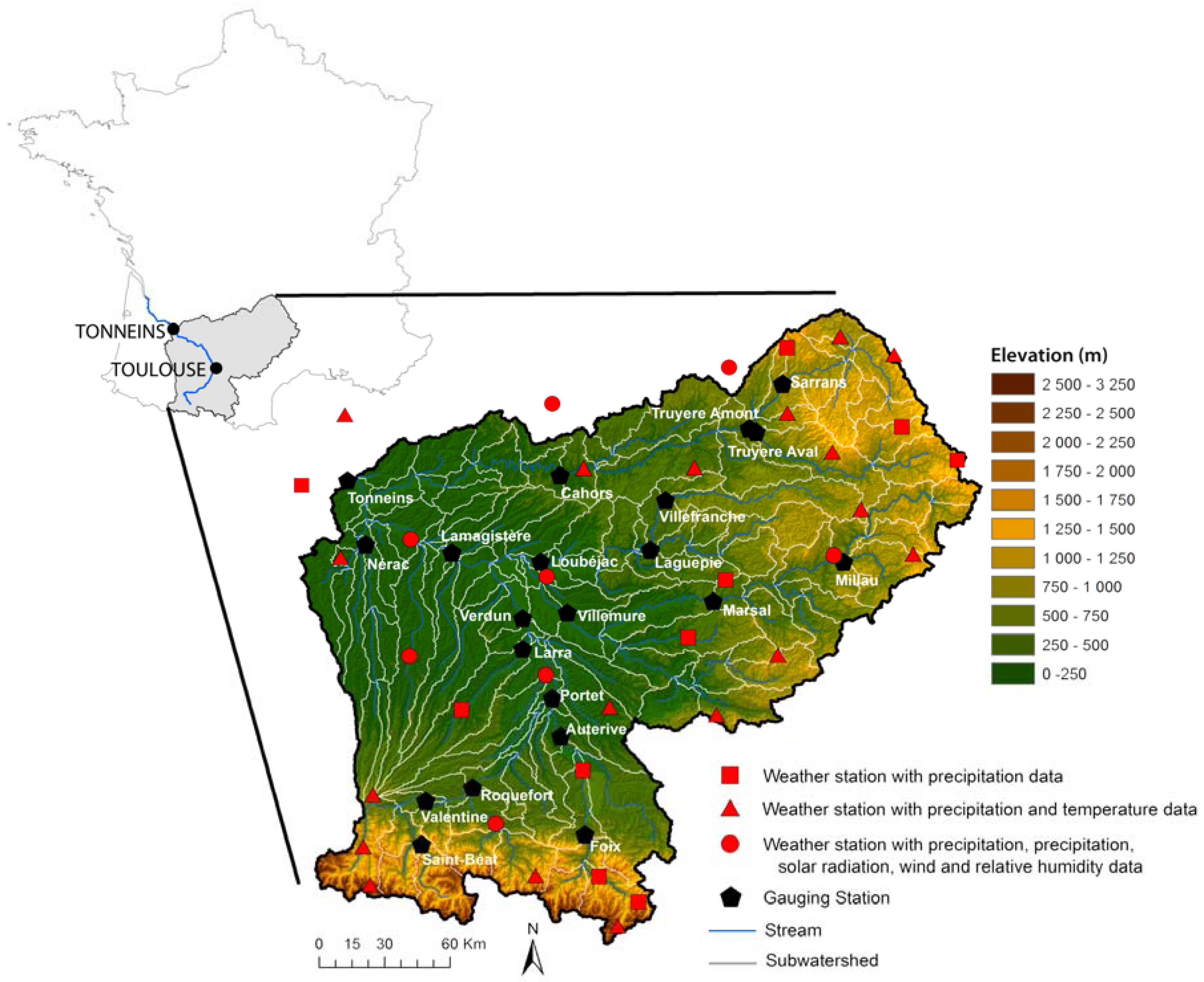
Data sources for this study are presented in
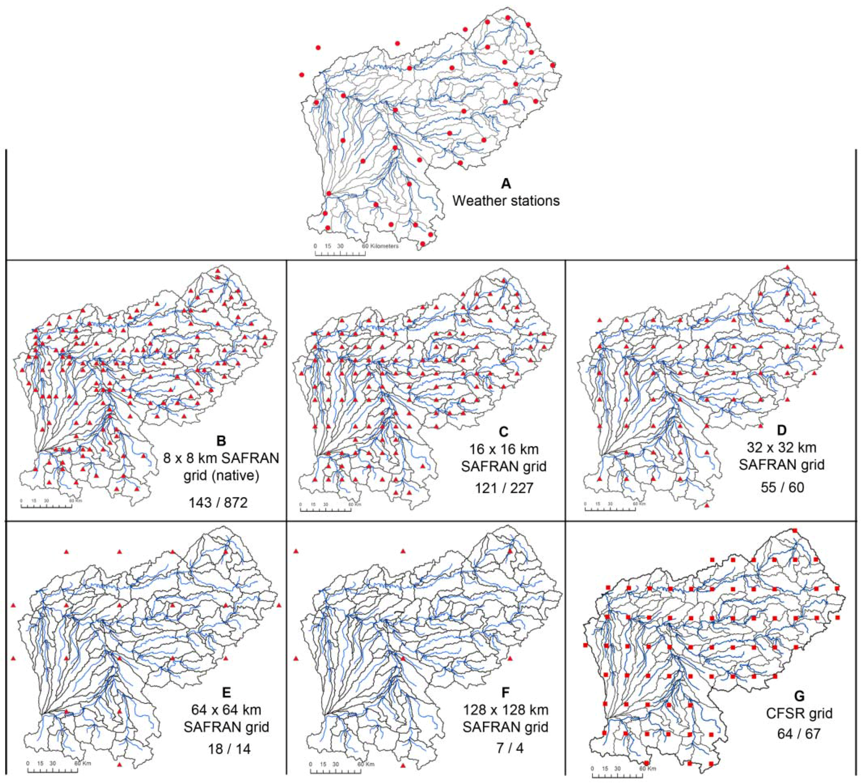
Table 1. River discharge data are available from 21 gauging stations spread over the watershed and covering the period from 2000 to 2010 (
Figure 1). Two climate datasets from Météo-France were compared: standard stations providing precipitation at 36 sites, temperature at 28 sites, and solar radiation, relative humidity and wind speed at eight sites (
Figure 1) and the 8-km SAFRAN product providing all of the required variables at each grid point [
9,
10,
11]. SAFRAN uses the optimal interpolation (OI) method [
31], which corrects background values against all nearby observed data, applying a linear regression in which observations are weighted by distance and associated error. In SAFRAN, the background values originate from the ARPEGE meteorological model from the French meteorological agency [
32] or the ECMWF operational archives, while the observations are from a large range of datasets, such as ground-based climate stations, snow monitoring networks, weather balloons and dropsondes.
The SAFRAN grid is constructed in three stages: interpolation of all atmospheric parameters to a 300-m vertical resolution, horizontal interpolation of the surface parameter and temporal interpolation. A more comprehensive description of this process is reported in Durand, Brun, Merindol, Guyomarch, Lesaffre and Martin [
9] and Quintana-Segui, Le Moigne, Durand, Martin, Habets, Baillon, Canellas, Franchisteguy and Morel [
10].
A second gridded climate product, the CFSR grid, was used in this comparison [
7]. Free access is now provided to SWAT users via the Texas A&M University spatial sciences website [
37] which automatically creates SWAT-formatted input files. The CFSR has latitudinal and longitudinal resolutions of 0.5°, which over the Garonne watershed correspond to a resolution of ~35-km in latitude and ~25-km in longitude. The CFSR was built around coupled atmospheric, oceanic and surface modelling components, corrected with satellite, aircraft, radiosonde, pibal and in situ data from both land and ocean [
7]. Like SAFRAN, the data are interpolated according to the OI method, as described in Xie, et al. [
39] for land surfaces and Reynolds, et al. [
40] for ocean surfaces.
2.4. Watershed Discretisation
As mentioned above, the SWAT model only uses one source of climate information per subwatershed: the one nearest to the centroid. The number of information points used by the model is therefore directly linked to the areal discretisation defined by the user during the SWAT implementation phase. However, the delineation of the subwatersheds was initially based on the need for a fair representation of all of the hydrological processes prevailing on the watershed and on computing time allocation. In this project, data presented in
Table 1 have been used to set up the SWAT model. The watershed was divided into 150 subbasins to allow the representation of the different hydrological behaviours highlighted by Probst [
24]. HRUs were defined on soil, land use and slope, retaining only information covering more than 10% of the subbasin area, as proposed by Srinivasan [
41].
2.5. Aggregation of the SAFRAN Product
In order to evaluate the spatial appropriateness of the SAFRAN 8-km product against the SWAT areal discretisation of the Garonne River watershed, other resolutions of the former were computed, aggregating the gridded information to 16, 32, 64 and 128 km, respectively.
All climate datasets, including information from the ground stations, were then used in turn to simulate the hydrology of the Garonne River. In the first step, a reference calibration was undertaken based on the ground stations (
Figure 1). SWAT was then run with the native SAFRAN product, the native CFSR product and all SAFRAN-aggregated grids. During the second stage, new calibrations were performed based on the native 8-km SAFRAN product and the SAFRAN product aggregated to 32 km (see
Section 3.1). In all instances, performance values were computed and compared for the 2000–2010 period at a monthly time step.
2.6. Sensitivity Analysis and Calibration Process
Sensitivity analysis and calibration were undertaken within SWAT-Cup [
42] using the SUFI-2 (Sequential Uncertainty Fitting 2) algorithm [
43]. SWAT-Cup is an external software tool that allows SWAT users to perform automatic calibrations [
44]. They are then given the option of several calibration algorithms, of which SUFI-2 is known to identify an appropriate parameter set in a limited number of iterations [
45].
A sensitivity analysis was performed, following the one-at-a-time procedure proposed by Abbaspour [
42]. Thirty two parameters were considered in the analysis (
Table 2). Five runs were performed over the 10-year period from 2000 to 2010, preceded by a three-year warming period (1997–2000).
Once the most sensitive parameters were identified (see
Supplementary Materials for more detail), 1500-run calibrations were performed as recommended by Yang, Reichert, Abbaspour, Xia and Yang [
45]. The SWAT-Cup calibration was achieved sequentially from upstream to downstream, one gauging station at the time, using the Nash–Sutcliffe efficiency criterion (NSe) [
47] as the objective function. NSe is a normalised metric allowing a comparison between the variance of the observed dataset and the existing variance of residual errors between this same observed dataset and the simulated one. It ranges from −∞ to 1 and is sensitive to large errors. It equals 0 when the model is as accurate as the mean of the observed dataset and equals 1 when the model offers a perfect fit.
After calibration, the performance was evaluated using the same criterion, but calculated on the root square of discharge values (NSeSqrt) in order to diminish the influence of large errors on the metric. Indeed, the NSeSqrt is influenced more greatly by common flows and the error on the global simulated volume [
48,
49].
3. Results and Discussion
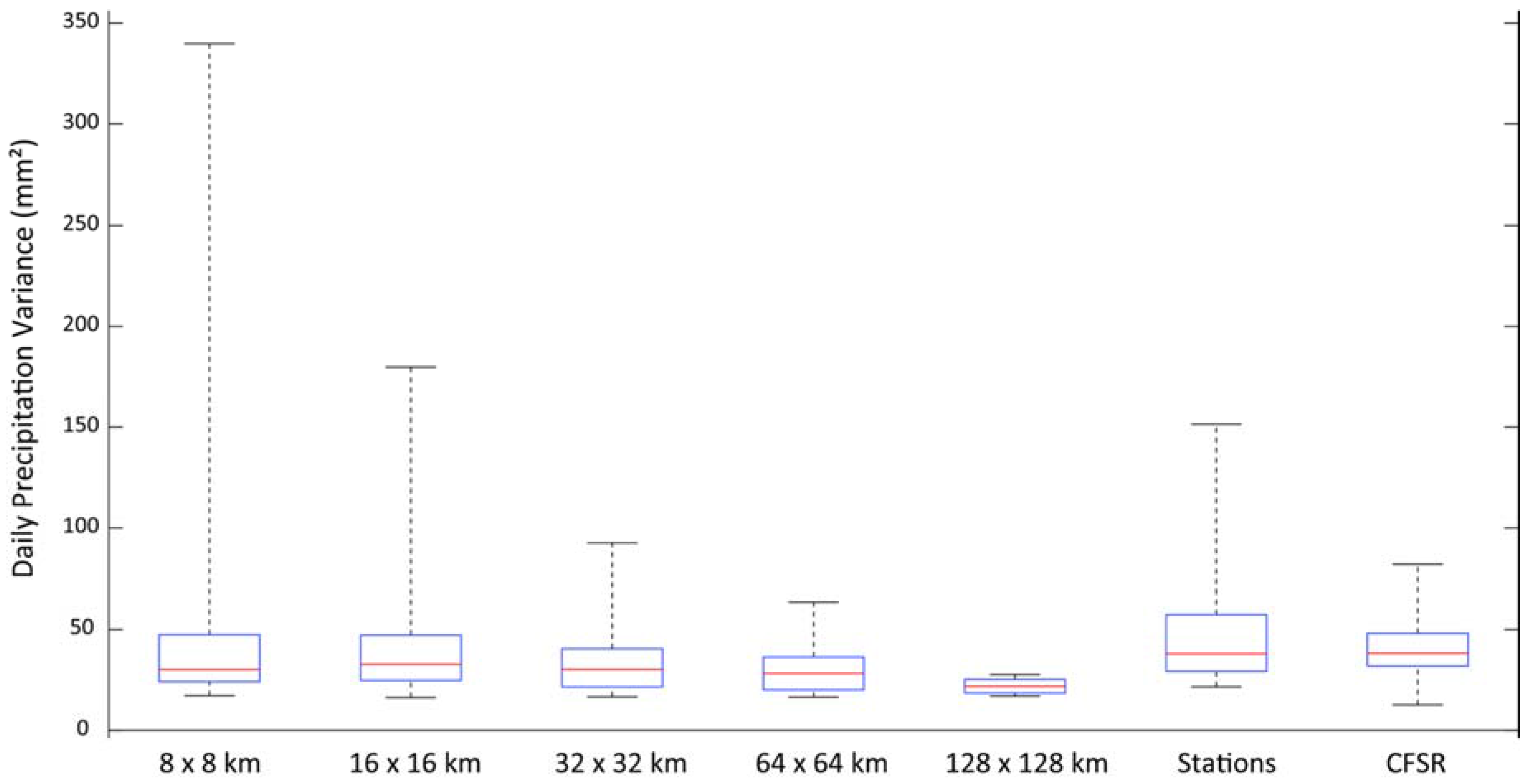
3.1. Climate Data of Different Resolutions
Seven climate datasets were compared for the Garonne River watershed: the network of standard ground stations, the 8-km SAFRAN product, SAFRAN aggregated to 16, 32, 64 and 128 km and the 30-km CFSR product. SAFRAN and CFSR come from a combination of meteorological simulations and observations and may therefore possess a different spatial variance than the network of ground stations. SAFRAN aggregation also results in a reduction in variance or, in other words, reduces its ability to describe irregular, non-uniform precipitation patterns [
50].
Ranges in the spatial variance of the daily precipitation are compared in
Figure 2 for the watershed of the Garonne River at Tonneins. As expected, aggregation smoothed out spatial irregularities, which is evident in
Figure 2 in the significant loss of large variance events when reducing the resolution from the initial 8 km to the aggregated 128 km. On the other hand, not all precipitation events are non-uniform, so it was mostly higher values of the variance distributions that were affected by the aggregation process.
Figure 2 also illustrates the spatial variance of the precipitation reported by the network of ground stations. The 8-km SAFRAN had a narrower and lower distribution and a lower median value than the network of stations, but the use of information from many different sources and an 8-km resolution allowed SAFRAN to report more irregular events. In practice, the variance of the network between the 16- and 32-km aggregated SAFRAN grids in terms of spatial variance was an indication of the factual resolution of the irregularly-spaced climate stations. Finally, the CFSR product offered yet another distribution of the spatial variance of daily precipitation, which lay between the aggregated 32-km and 64-km SAFRAN grids.
The fact that the choice was made to break down the watershed into 150 subwatersheds limited the number of local climate information points to 150 and raised the question of the optimal resolution of climate data. Indeed, too high a resolution forced SWAT to disregard much of the information, and too low a resolution forced SWAT to use the same information for many adjacent subwatersheds, whereas the resolution of the climate grid had a direct influence on its ability to describe non-uniformities in the precipitation patterns, as mentioned above. This issue is illustrated in
Figure 3, which shows points of local climate information used by SWAT. It is evident that SWAT was not able to make use of all of the 8-km information; it used most of the 16-km information and used nearly all of the information from a resolution of 32-km and more. From this perspective, the 32-km SAFRAN grid was the closest to the resolution of the station network, as was the 30-km CFSR product.
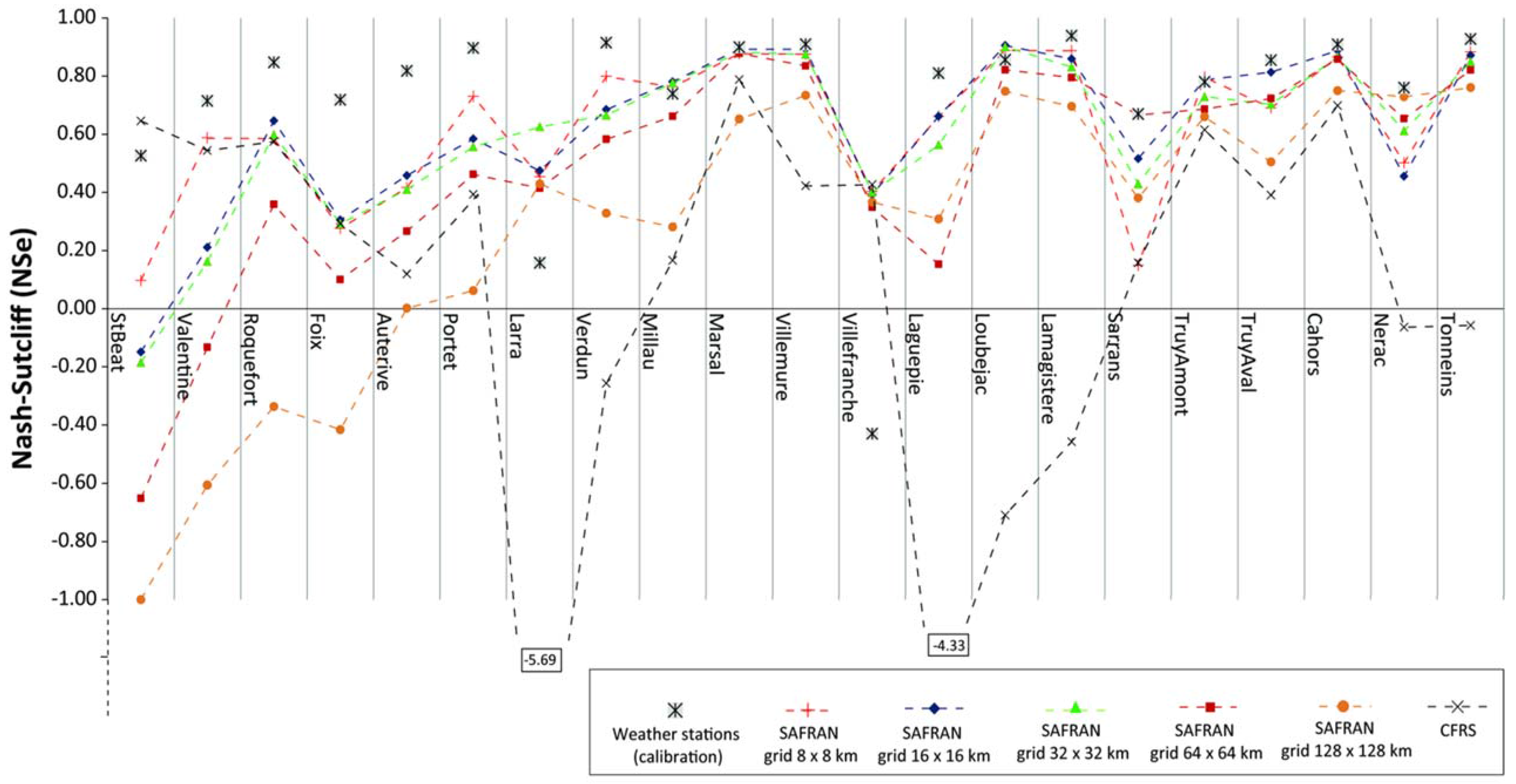
3.2. Hydrological Performance
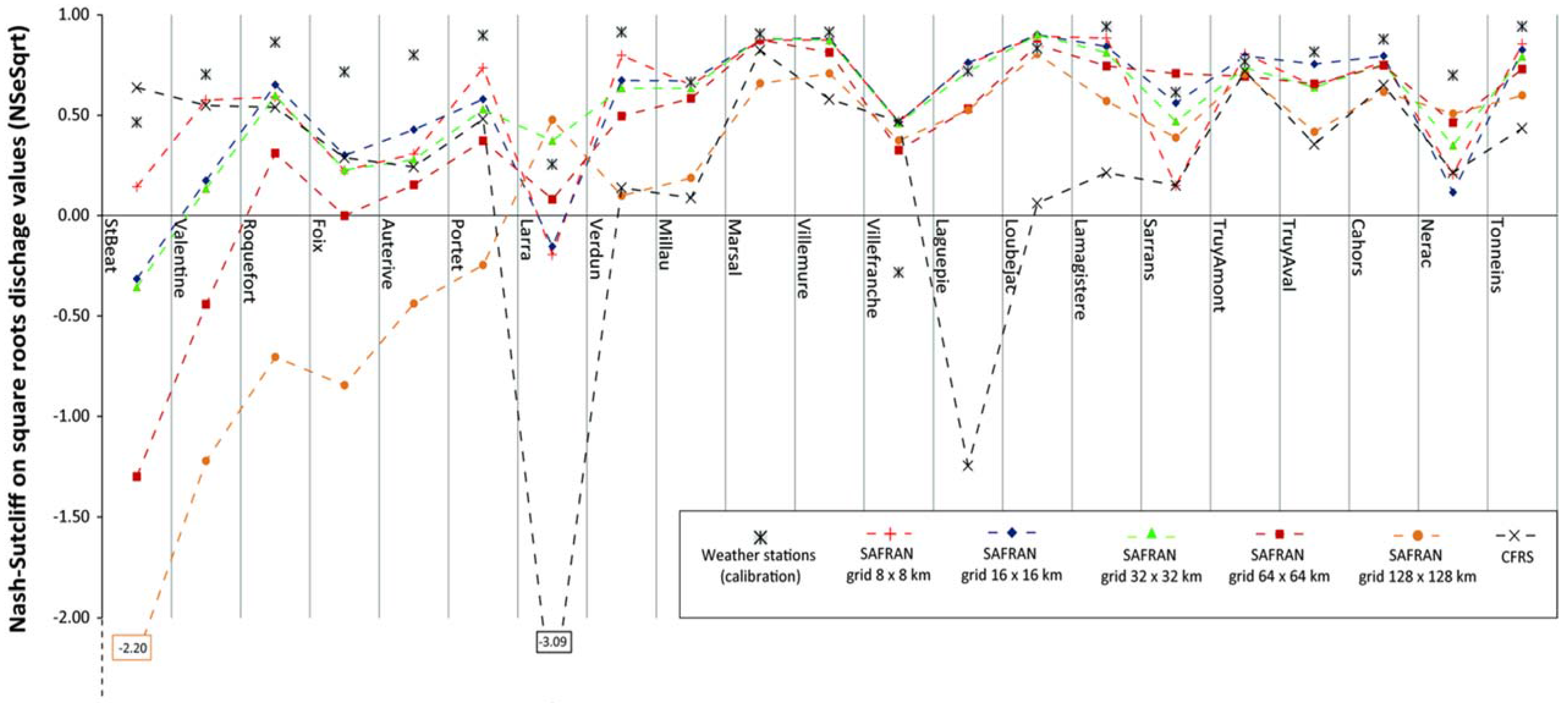
Figure 4 and
Figure 5 compare the performance values (NSe and NSeSqrt) of the SWAT model calibrated with the network of ground stations and run with each SAFRAN grid and the CFSR grid (values of the calibrated parameters can be found in the
Supplementary Materials). Using the data from SAFRAN did not improve on the network of ground stations, except at two sites, Larra and Villefranche, where the initial performance was unsatisfactory. Excessive aggregation was detrimental to SWAT performance, as depicted by the much lower SWAT performance when operated with the 64- or 128-km SAFRAN grids, while the other three resolutions were closer to one another in terms of performance.
CFSR data produced heterogeneous performances, mostly similar to those obtained with the 8-, 16- and 32-km SAFRAN grids, and was even better than in the calibration for the St Béat station (see
Figure 1), but also for stations where the SWAT model completely failed to simulate the discharge. When comparing different products, the fact that 8-, 16- and 32-km SAFRAN grids produced similar performances, which were worse than the weather station data and for several stations, very different from the CFSR performance values, indicated that it was not so much an issue of spatial resolution than one of a different representation of the climate.
It is noteworthy that the performance of the Saint Béat and Valentine gauging stations declined as the aggregation increased. Both stations are located in the Pyrenean part of the watershed, where the model is quite sensitive to the snow-relative calibration [
28].
As for the Larra and Villefranche sites, each site drains a single subwatershed, where no merging with other subwatersheds can compensate for any errors in a climate series. These poor performance values may also be a representation of a widespread problem when using in situ gauging stations: weather data used to compute hydrological processes in a subwatershed could originate from a distant gauging station and may not be representative of the subwatershed [
13]. Indeed, when the weather stations’ datasets were used in the SWAT model, computations in subwatersheds upstream of the Villefranche and Truyère-Amont sites were performed using the same weather station, located in the subwatershed upstream of the Truyère-Amont station (
Figure 1). Unlike the Villefranche site, no important loss in performance at Truyère-Amont was seen, suggesting that even though the weather station was located close to the Villefranche watershed, it was not representative of that particular system.
As for the CFSR grid, it proposed non-representative precipitation data in some areas. Indeed, a detailed analysis of the hydrographs (not illustrated) revealed that CFSR forced SWAT to overestimate discharges greatly at Larra and Laguepie, a problem that was then transmitted downstream to Verdun, Loubéjac, Lamagistère and Tonneins, while discharge was underestimated at Millau and Sarrans. When comparing hydrographs and hyetographs, it appeared that overestimations were mainly caused by grid points where precipitation was overestimated when compared to the rest of the grid. This was consistent with the findings of Dile and Srinivasan [
15], who encountered the same situation over the Blue Nile watershed.
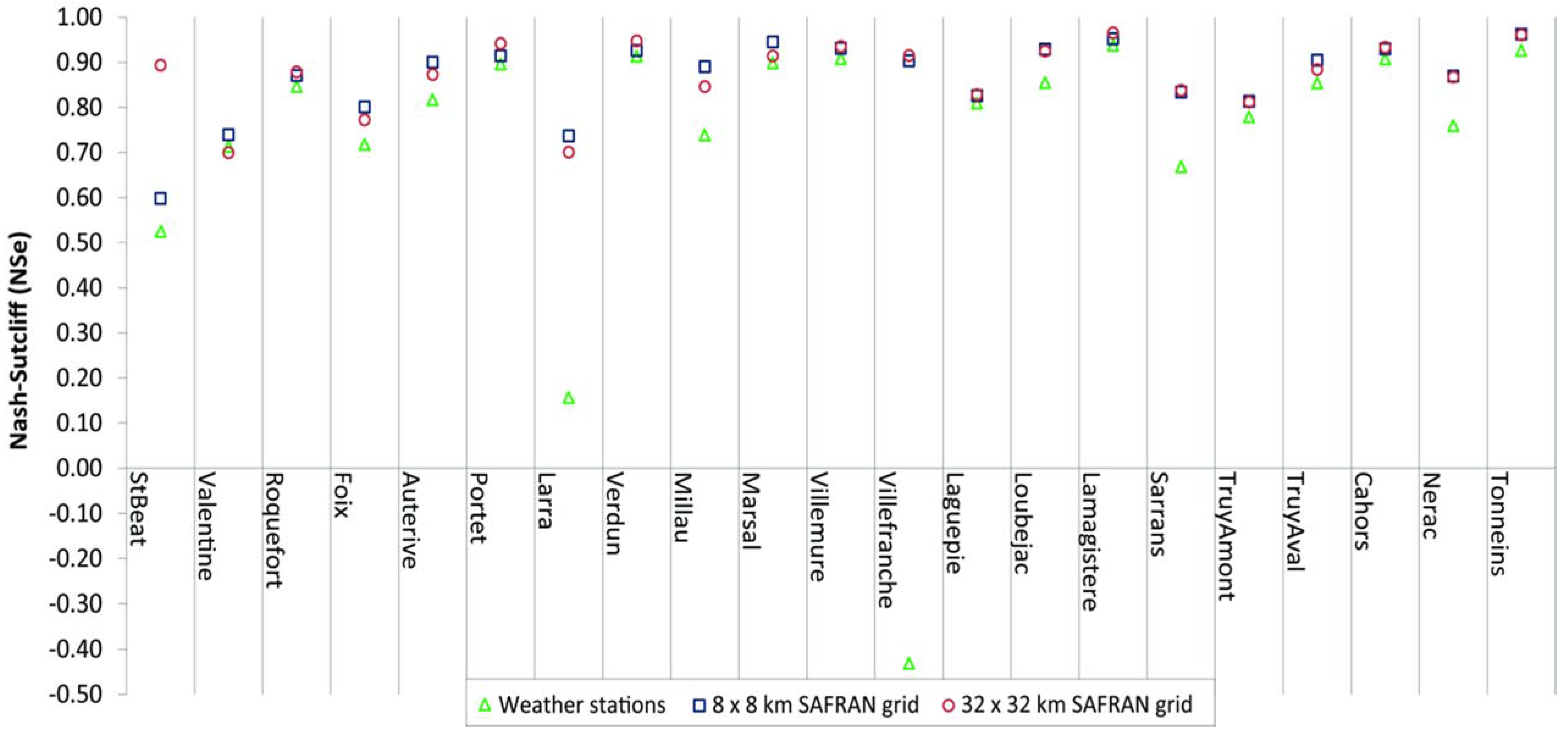
In order to document the issue of SAFRAN and the network of stations not reporting exactly the same climatology, it was decided to recalibrate SWAT alternately using the 8- and 32-km SAFRAN grids, since the 8-km resolution described spatial non-uniformity better, and the 32-km resolution was the closest to the network’s (values of calibrated parameters are provided as
Supplementary Materials).
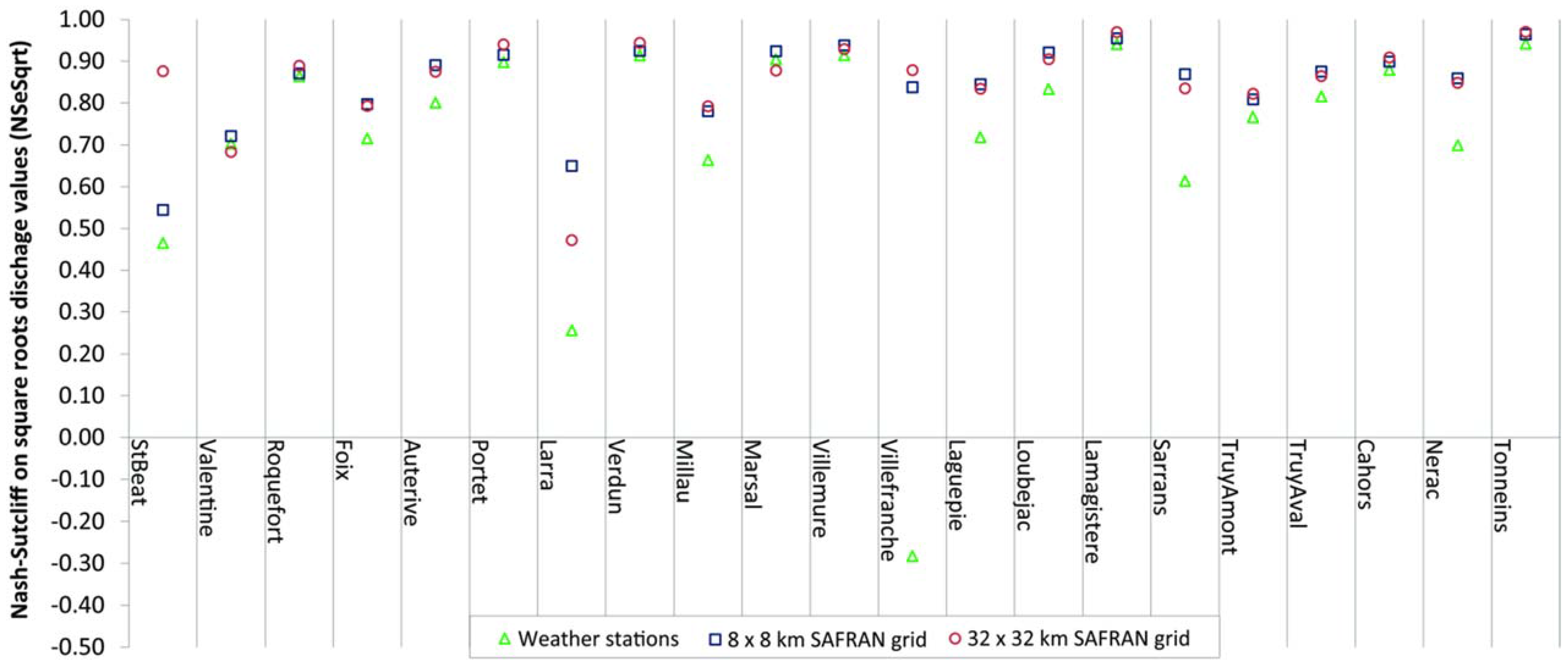
Here,
Figure 6 and
Figure 7 show poorer SWAT performance values when calibrated with the network of climate stations than with any of the two SAFRAN grids, which was consistent with previous studies [
13,
18]. Better performance values at the Larra and Villefranche sites when using SAFRAN tended to confirm that, at least for these two sites, climate stations were either non-representative or included errors. Moreover, the performance at Tonneins, which integrates climate data across the entire watershed, confirmed the superiority of the SAFRAN product. This highlights the benefit of using a gridded dataset developed from the interpolation and cross-checking of weather data, which avoids temporal gaps, is less influenced by very local events and guarantees space-time consistency for all meteorological variables [
11].
The performance of the 8- and 32-km SAFRAN grids was mostly similar, indicating that the grid resolution did not have a considerable influence on the calibration. The largest gain was at Saint Béat in the Pyrenees, where the 32-km resolution proved to be quite beneficial, as it was for the CFSR dataset.
In this case, the Pyrenean gauging stations do not behave differently from the other ones, in opposition to the previous modelling step when running SWAT (reference calibration) with the various upscale grids, which led to a loss in performance values at those sites. Moreover, for some of them (St Beat, Roquefort and Portet), a gain in performance is obtained. These results confirmed the capacity of the calibration to take full advantage of the available information, especially in mountainous regions.
4. Conclusions
The implementation of a semi-distributed hydrological model generally involves breaking down the watershed space into homogeneous units that are compatible with the dynamic computation of the hydrological processes. In the case of the SWAT model, only one climate grid point per subwatershed, the nearest one, was used for the calculations, raising the question of the optimal resolution of the climate data. In this study, the 45,000-km2 Garonne River watershed at Tonneins, which drains a substantial part of southwest France to the Atlantic Ocean, was used to compare three sources of climate information in different formats and resolutions, namely the available climate station network, the 8-km SAFRAN product and the ~30-km CFSR product. SAFRAN grids aggregated to 16, 32, 64 and 128 km were also explored.
A spatial breakdown of the Garonne watershed into 150 subwatersheds was deemed as optimal to represent the hydrological functioning of the catchment, as well as adequate regarding to computing costs. From this breakdown results also the limitation of the number of local climate grid points to 150. A higher climate data resolution would therefore force SWAT to disregard much of the information, and a much lower resolution would force SWAT to use the same information for many adjacent subwatersheds, whereas the resolution of the climate grid had a direct influence on its ability to describe non-uniformities in the precipitation patterns.
The results showed that aggregating SAFRAN up to 64 or 128 km was detrimental to the description of non-uniform precipitation events, to the point of leading to a much poorer performance when used with the SWAT implementation calibrated on the available network of climate stations. The native 8-km SAFRAN product offered the variability of daily precipitation events, while the aggregated 16- and 32-km SAFRAN grids and the ~30-km CFSR product ranges of spatial variance were similar to that of the network of climate stations.
Running the SWAT model calibrated on the network of climate stations with the 8-, 16- and 32-km SAFRAN grids led to very similar performance values at most sites, but lower than those previously obtained in calibration. These results suggest that the difference in the representation of the climate was more influential than its spatial resolution in simulating the hydrological processes within the SWAT model. Using CFSR with the same framework provided similar overall performance values as SAFRAN for some sites, but for others, CFSR provided precipitation rates that were judged to be unrealistic when compared to the other climate databases.
The great importance of the quality of the climate product over its resolution was confirmed when calibrating SWAT with the native 8-km SAFRAN and its aggregated 32-km counterpart, since both of these datasets led to very similar performances that were better overall than the calibration performance values previously obtained by calibrating SWAT with the network of climate stations.
Results obtained in this study are consistent with previous works revealing the benefit of using a gridded dataset. However, the choice of the dataset is influenced by (1) the resolution range, which must be adapted to the model definition, even if certain resolution seems to lead to similar performance values, and (2) the representation of the climate by the dataset. It is thus quite important to select a dataset that is suitable to the model and to the climatological characteristics of the watershed.
The present study was based on monthly time step performance computations, compatible with water planning needs, where the influences of extreme precipitation are limited. An equivalent study calculating performances at a daily time step could generate additional findings that could have flood warning applications.
Acknowledgments
The authors acknowledge the financial support given by the Natural Sciences and Engineering Research Council of Canada and the Institut Hydro-Québec en environnement, développement et société. This research was carried out as a part of the ADAPT’EAU project (Adaptation aux variations des régimes hydrologiques-ANR-11-CEPL-008), a project supported by the French National Research Agency (ANR—Agence Nationale de la Recherche) within the framework of the Global Environmental Changes and Societies (GEC&S) programme. This work was also part of the REGARD project (modélisation des REssources en eau sur le bassin de la GAronne: interaction entre les composantes naturelles et anthropiques et apport de la téléDétection) funded by the RTRA-STAE (Réseau Thématique de Recherche Avancées-Sciences et Technologies pour l’Aéronautique et l’Espace)—2014–2017. We sincerely thank Météo-France for providing meteorological data and AEAG (Agence de l’Eau Adour-Garonne) for providing hydrological discharge data.
Author Contributions
Youen Grusson conceived of, designed, performed the experiments and wrote the paper as part of his Ph.D. thesis. François Anctil and José Miguel Sánchez Pérez supervised the Ph.D. candidate. Sabine Sauvage also provided help throughout the work. All coauthors have collaborated on the redaction of the manuscript.
Conflicts of Interest
The authors declare no conflict of interest.
References
- Arnold, J.G.; Allen, P.M.; Bernhardt, G. A comprehensive surface-groundwater flow model. J. Hydrol. 1993, 142, 47–69. [Google Scholar] [CrossRef]
- Srinivasan, R.; Ramanarayanan, T.S.; Arnold, J.G.; Bednarz, S.T. Large area hydrologic modeling and assessment part II: Model application. J. Am. Water Resour. Assoc. 1998, 34, 91–101. [Google Scholar] [CrossRef]
- Arnold, J.G.; Srinivasan, R.; Muttiah, R.S.; Williams, J.R. Large area hydrologic modeling and assessment part I: Model development. J. Am. Water Resour. Assoc. 1998, 34, 73–89. [Google Scholar] [CrossRef]
- Gassman, P.W.; Reyes, M.R.; Green, C.H.; Arnold, J.G. The soil and water assessment tool: Historical development, applications, and future research directions. Trans. ASABE 2007, 50, 1211–1250. [Google Scholar] [CrossRef]
- Douglas-Mankin, K.R.; Srinivasan, R.; Arnold, J.G. Soil and water assessment tool (SWAT) model: Current developments and applications. Trans. ASABE 2010, 53, 1423–1431. [Google Scholar] [CrossRef]
- Gassman, P.W.; Sadeghi, A.M.; Srinivasan, R. Applications of the SWAT model special section: Overview and insights. J. Environ. Qual. 2014, 43, 1–8. [Google Scholar] [CrossRef] [PubMed]
- Saha, S.; Moorthi, S.; Pan, H.-L.; Wu, X.; Wang, J.; Nadiga, S.; Tripp, P.; Kistler, R.; Woollen, J.; Behringer, D.; et al. The NCEP climate forecast system reanalysis. Bull. Am. Meteorol. Soc. 2010, 91, 1015–1057. [Google Scholar] [CrossRef]
- Uppala, S.M.; Kallberg, P.W.; Simmons, A.J.; Andrae, U.; Bechtold, V.D.C.; Fiorino, M.; Gibson, J.K.; Haseler, J.; Hernandez, A.; Kelly, G.A.; et al. The ERA-40 re-analysis. Q. J. R. Meteorol. Soc. 2005, 131, 2961–3012. [Google Scholar] [CrossRef]
- Durand, Y.; Brun, E.; Merindol, L.; Guyomarch, G.; Lesaffre, B.; Martin, E. A meteorological estimation of relevant parameters for snow models. Ann. Glaciol. 1993, 18, 65–71. [Google Scholar]
- Quintana-Segui, P.; Le Moigne, P.; Durand, Y.; Martin, E.; Habets, F.; Baillon, M.; Canellas, C.; Franchisteguy, L.; Morel, S. Analysis of near-surface atmospheric variables: Validation of the SAFRAN analysis over France. J. Appl. Meteorol. Clim. 2008, 47, 92–107. [Google Scholar] [CrossRef]
- Vidal, J.P.; Martin, E.; Franchisteguy, L.; Baillon, M.; Soubeyroux, J.M. A 50-year high-resolution atmospheric reanalysis over France with the SAFRAN system. Int. J. Climatol. 2010, 30, 1627–1644. [Google Scholar] [CrossRef]
- Livneh, B.; Bohn, T.J.; Pierce, D.W.; Munoz-Arriola, F.; Nijssen, B.; Vose, R.; Cayan, D.R.; Brekke, L. A spatially comprehensive, hydrometeorological data set for Mexico, the U.S., and Southern Canada 1950–2013. Sci. Data 2015, 2. [Google Scholar] [CrossRef] [PubMed]
- Fuka, D.R.; Walter, M.T.; MacAlister, C.; Degaetano, A.T.; Steenhuis, T.S.; Easton, Z.M. Using the climate forecast system reanalysis as weather input data for watershed models. Hydrol. Process. 2014, 28, 5613–5623. [Google Scholar] [CrossRef]
- Auerbach, D.A.; Easton, Z.M.; Walter, M.T.; Flecker, A.S.; Fuka, D.R. Evaluating weather observations and the climate forecast system reanalysis as inputs for hydrologic modelling in the tropics. Hydrol. Process. 2016, 30, 3466–3477. [Google Scholar] [CrossRef]
- Dile, Y.T.; Srinivasan, R. Evaluation of CFSR climate data for hydrologic prediction in data-scarce watersheds: An application in the Blue Nile River Basin. J. Am. Water Resour. Assoc. 2014, 50, 1226–1241. [Google Scholar] [CrossRef]
- Monteiro, J.A.F.; Strauch, M.; Srinivasan, R.; Abbaspour, K.; Gücker, B. Accuracy of grid precipitation data for Brazil: Application in river discharge modelling of the Tocantins catchment. Hydrol. Process. 2016, 30, 1419–1430. [Google Scholar] [CrossRef]
- Weedon, G.P.; Balsamo, G.; Bellouin, N.; Gomes, S.; Best, M.J.; Viterbo, P. The WFDEI meteorological forcing data set: Watch forcing data methodology applied to ERA-interim reanalysis data. Water Resour. Res. 2014, 50, 7505–7514. [Google Scholar] [CrossRef]
- de Almeida Bressiani, D.; Srinivasan, R.; Jones, C.A.; Mendiondo, E.M. Effects of different spatial and temporal weather data resolutions on the streamflow modeling of a semi-arid basin, Northeast Brazil. Int. J. Agric. Biol. Eng. 2015, 8, 125–139. [Google Scholar]
- Chaplot, V.; Saleh, A.; Jaynes, D.B. Effect of the accuracy of spatial rainfall information on the modeling of water, sediment, and NO3-N loads at the watershed level. J. Hydrol. 2005, 312, 223–234. [Google Scholar] [CrossRef]
- Cho, H.D.; Olivera, F. Effect of the spatial variability of land use, soil type, and precipitation on streamflows in small watersheds. J. Am. Water Resour. Assoc. 2009, 45, 673–686. [Google Scholar] [CrossRef]
- Masih, I.; Maskey, S.; Uhlenbrook, S.; Smakhtin, V. Assessing the impact of areal precipitation input on streamflow simulations using the SWAT model. J. Am. Water Resour. Assoc. 2011, 47, 179–195. [Google Scholar] [CrossRef]
- Shope, C.L.; Maharjan, G.R. Modeling spatiotemporal precipitation: Effects of density, interpolation, and land use distribution. Adv. Meteorol. 2015. [Google Scholar] [CrossRef]
- Cho, J.; Bosch, D.; Lowrance, R.; Strickland, T.; Vellidis, G. Effect of spatial distribution of rainfall on temporal and spatial uncertainty of SWAT output. Trans. ASABE 2009, 52, 1545–1555. [Google Scholar] [CrossRef]
- Probst, J.L. Hydrologie du Bassin de la Garonne: Modèles de Mélange, Bilan de l’Erosion, Exportation des Nitrates et des Phosphates; University of Toulouse: Toulouse, France, 1983. (In French) [Google Scholar]
- Ferrant, S.; Oehler, F.; Durand, P.; Ruiz, L.; Salmon-Monviola, J.; Justes, E.; Dugast, P.; Probst, A.; Probst, J.L.; Sanchez-Perez, J.M. Understanding nitrogen transfer dynamics in a small agricultural catchment: Comparison of a distributed (TNT2) and a semi distributed (SWAT) modeling approaches. J. Hydrol. 2011, 406, 1–15. [Google Scholar] [CrossRef]
- Boithias, L.; Sauvage, S.; Taghavi, L.; Merlina, G.; Probst, J.L.; Perez, J.M.S. Occurrence of metolachlor and trifluralin losses in the save river agricultural catchment during floods. J. Hazard. Mater. 2011, 196, 210–219. [Google Scholar] [CrossRef] [PubMed]
- Oeurng, C.; Sauvage, S.; Sanchez-Perez, J.M. Assessment of hydrology, sediment and particulate organic carbon yield in a large agricultural catchment using the SWAT model. J. Hydrol. 2011, 401, 145–153. [Google Scholar] [CrossRef]
- Grusson, Y.; Sun, X.; Gascoin, S.; Sauvage, S.; Raghavan, S.; Anctil, F.; Sanchez Pérez, J.M. Assessing the capability of the SWAT model to simulate snow, snow melt and streamflow dynamics over an alpine watershed. J. Hydrol. 2015, 531, 574–588. [Google Scholar] [CrossRef]
- Olivera, F.; Valenzuela, M.; Srinivasan, R.; Choi, J.; Cho, H.; Koka, S.; Agrawal, A. Arcgis-SWAT: A geodata model and GIS interface for SWAT. J. Am. Water Resour. Assoc. 2006, 42, 295–309. [Google Scholar] [CrossRef]
- SWAT Documentation Web Page. Available online: http://swat.tamu.edu/documentation/ (accessed on 10 December 2016).
- Gandin, L.S. Objective Analysis of Meteorological Fields; Gidrometeorologicheskoe Izdatelstvo: Leningrad, Russian, 1963. (In Russian) [Google Scholar]
- Courtier, P.; Freydier, C.; Geleyn, J.; Rabier, F.; Rochas, M. The Arpege Project at Meteo-France. Available online: http://www.ecmwf.int/sites/default/files/elibrary/1991/8798-arpege-project-meteo-france.pdf (accessed on 13 January 2017).
- NASA; JPL. ASTER—Global Digital Elevation Model v2 90 × 90 m. 2011. Available online: https://asterweb.jpl.nasa.gov/gdem.asp (accessed on 15 January 2017). [Google Scholar]
- Corine Land Cover; European Union: Brussels, Belgium, 2006; Available online: http://land.copernicus.eu/pan-european/corine-land-cover (accessed on 15 January 2017).
- European Soil Data Base v2.0, 1 km × 1 km “Dominant Value and Dominant Stu” Rasters EEA; European Union: Brussels, Belgium, 2006; Available online: https://eusoils.jrc.ec.europa.eu (accessed on 15 January 2017).
- Météo France Data Services. Available online: https://donneespubliques.meteofrance.fr/ (accessed on 22 November 2014).
- Global Weather Data for SWAT. Available online: http://globalweather.tamu.edu/ (accessed on 10 December 2015).
- Banque Hydro. Available online: http://www.hydro.eaufrance.fr/ (accessed on 13 November 2014).
- Xie, P.; Chen, M.; Yang, S.; Yatagai, A.; Hayasaka, T.; Fukushima, Y.; Liu, C. A gauge-based analysis of daily precipitation over East Asia. J. Hydrometeorol. 2007, 8, 607–626. [Google Scholar] [CrossRef]
- Reynolds, R.W.; Smith, T.M.; Liu, C.; Chelton, D.B.; Casey, K.S.; Schlax, M.G. Daily high-resolution-blended analyses for sea surface temperature. J. Clim. 2007, 20, 5473–5496. [Google Scholar] [CrossRef]
- Srinivasan, R. Soil and Water Assessment Tool—Introductory Manual—Version 2012. Available online: http://swat.tamu.edu/documentation/ (accessed on 10 September 2014).
- Abbaspour, K.C. SWAT-CUP 2012: SWAT Calibration and Uncertainty Programs—A User Manual; EAWAG: Dübendof, Switzerland, 2013; p. 103. [Google Scholar]
- Abbaspour, K.C.; Johnson, C.A.; van Genuchten, M.T. Estimating uncertain flow and transport parameters using a sequential uncertainty fitting procedure. Vadose Zone J. 2004, 3, 1340–1352. [Google Scholar] [CrossRef]
- Arnold, J.G.; Moriasi, D.N.; Gassman, P.W.; Abbaspour, K.C.; White, M.J.; Srinivasan, R.; Santhi, C.; Harmel, R.D.; van Griensven, A.; van Liew, M.W.; et al. SWAT: Model use, calibration, and validation. Trans. ASABE 2012, 55, 1491–1508. [Google Scholar] [CrossRef]
- Yang, J.; Reichert, P.; Abbaspour, K.C.; Xia, J.; Yang, H. Comparing uncertainty analysis techniques for a SWAT application to the Chaohe Basin in China. J. Hydrol. 2008, 358, 1–23. [Google Scholar] [CrossRef]
- Arnold, J.G.; Kiniry, J.R.; Srinivasan, R.; Williams, J.R.; Haney, E.B.; Neitsch, S.L. Soil and Water Assessment Tool—Input/Output Documentation—Version 2012. Available online: http://swat.tamu.edu/documentation/ (accessed on 16 January 2016).
- Nash, J.E.; Sutcliffe, J.V. River flow forecasting through conceptual models part I—A discussion of principles. J. Hydrol. 1970, 10, 282–290. [Google Scholar] [CrossRef]
- Oudin, L.; Andréassian, V.; Mathevet, T.; Perrin, C.; Michel, C. Dynamic averaging of rainfall-runoff model simulations from complementary model parameterizations. Water Resour. Res. 2006. [Google Scholar] [CrossRef]
- Seiller, G.; Anctil, F.; Perrin, C. Multimodel evaluation of twenty lumped hydrological models under contrasted climate conditions. Hydrol. Earth Syst. Sci. 2012, 16, 1171–1189. [Google Scholar] [CrossRef]
- Gaborit, É.; Anctil, F.; Fortin, V.; Pelletier, G. On the reliability of spatially disaggregated global ensemble rainfall forecasts. Hydrol. Process. 2013, 27, 45–56. [Google Scholar] [CrossRef]
© 2017 by the authors; licensee MDPI, Basel, Switzerland. This article is an open access article distributed under the terms and conditions of the Creative Commons Attribution (CC-BY) license (http://creativecommons.org/licenses/by/4.0/).


