Flow Patterns and Morphological Changes in a Sandy Meander Bend during a Flood—Spatially and Temporally Intensive ADCP Measurement Approach

Abstract

The fluvio-geomorphological processes in meander bends are spatially uneven in distribution. Typically, higher velocities and erosion take place near the outer bank beyond the bend apex, while the inner bend point bar grows laterally towards the outer bank, increasing the bend amplitude. These dynamics maintain the meander evolution. Even though this development is found in meandering rivers independent of soil or environmental characteristics, each river still seems to behave unpredictably. The special mechanisms that determine the rate and occasion of morphological changes remain unclear. The aim of this study is to offer new insights regarding flow-induced morphological changes in meander using a novel study approach. We focused on short-term and small-spatial-scale changes by conducting a spatially and temporally (daily) intensive survey during a flood (a period of nine days) with an ADCP attached to a remotely controlled mini-boat. Based on our analysis, the flood duration and the rate of discharge increase and decrease seems to play key roles in determining channel changes by controlling the flow velocities and depth and the backwater effect may have notable influence on the morphological processes. We discuss themes such as the interaction of inner and outer bend processes and the longer-term development of meander bends.

1. Introduction

Morphological processes in rivers may have significant effects on both the environment and society. To be able to understand future river dynamics, present processes need to be investigated. A deeper understanding of fluvial processes and the ability to predict future evolution can be useful for example in river engineering, land use planning and river restoration.

Until recently, the field-based studies of river dynamics have been mostly realized along series of cross-sections over the river, the locations of which depended on the research question [1,2,3,4,5]. Therefore, the fundamental theories of the meander bends fluvio-geomorphology are also based on intensive cross-section based field studies performed during 1970s and 1980s [1,2,6,7,8,9,10,11]. These studies provided a strong basis for the understanding of the complex processes of meander bends and, thus, this period was followed by a relatively quiet era in field-based meandering research. The traditionally used cross-sectional measurements of the river geometry, however, may lead to a discontinuous picture of the river reach and may lead to an incorrect interpretation of the phenomenon [12,13,14,15,16]. Further, the cross-sectional measurements are time consuming and during the long-duration measurements, flow conditions may change between the first and the last measurement [17]. One of the main challenges for the empirical surveys has been how to achieve sufficient temporal resolution to study rapidly evolving fluvial processes and forms in the required level of detail [16,18]. In addition, the bathymetric surveys suffer from lower spatial resolution and accuracy compared to the topographical surveys [19,20]. This is why, in the wake of new technological developments during the 21st century, an increasing number of studies aiming of deepening the understanding of meander dynamics and challenging the fundamental theories of meandering rivers have been published.

Various recent studies have exploited modern measurement and modeling techniques such as terrestrial laser scanning [21,22], computational fluid dynamics [21,23,24] acoustic methods [25] and aerial photographs [26] in elucidating sub-bend scale meander dynamics. Due to the improved spatial and temporal resolution, the researchers have been able to highlight the diversity and variability of the fluvial and geomorphological processes that appear in meandering rivers in space and time. It has been shown, for example, that the processes in meandering rivers are episodic and not simply related to discharge, even though they exhibit an autogenic sequence described in qualitative models of meander development [26]. Kasvi et al. [21] showed that the influence of a flood on point bar evolution depends on the stage of the bend’s development, and that different parts of the point bars experience both erosion and deposition during a flood regardless of the final morphological changes. Engel and Rhoads [25] made important findings related to the processes in natural rivers. They stated that even though bank erosion andchannel migration are governed by near-bank velocity and turbulence, the flow patterns are influenced by the morphological characteristics of the bend, which may vary considerably. These include, for example, failed bank blocs which may inhibit the development of high near-bank velocities or, by contrast, increase the local shear stresses and rates of erosion [27]. These processes are, on the other hand, highly related to bank roughness and vegetation [27]. Ottewanger et al. [24] demonstrated that major differences exist between the hydrodynamic processes in mildly and sharply curved bends. There is also an ongoing debate about whether increases in bend sinuosity are led by inner bank push or outer bank pull. Various studies have stated that outer bank erosion is the leading process in meander migration, followed by point-bar growth and bar–floodplain conversion [28,29,30,31]. Recently, however, Schuurman et al. [32] stated, based on three numerical morphodynamic models, that bar–floodplain conversion, or “inner bank push”, is required for the development of high-sinuosity meanders with neck cutoffs. They deduced that sinuosity and specific conditions such as an outer bank’s erodibility may diminish the necessity of the inner bank push and thus explain the contradiction in the results. It is evident that the numerical models do not take into account the various factors that affect these processes in nature.

Thus far, however, no field-based study has measured daily geometric changes of a meander bend simultaneously with flow characteristics, to illustrate the spatial and temporal patterns of the processes and how they are related to the total change caused by a flood. Recently, there have been attempts to survey the flow field and morphology in high resolution with spatially continuous Acoustic Doppler Current Profiler (ADCP) data [33,34,35]. Flener et al. [33] demonstrated a measurement approach in which the ADCP device was attached to a remotely controlled mini-boat that was equipped with RTK-GNSS. The approach allowed for spatially dense flow and bed-level measurements in a relatively short period of time. They completed a spatially (0.2–1.1 points/m²) and temporally intensive ADCP measurement campaign over a highly mobile meander bend, 230 m in length and 20 to 55 m in width, during a flood event. They performed their daily survey nine times during one flood event, capturing both the rising and the descending limbs of the flood. However, no scientific research has yet exploited spatially continuous ADCP data to analyze the flow patterns and morphological changes of a meander bend. Thus, the data set collected and analyzed by Flener et al. [33] is used in this paper.

We will provide new insights regarding the flow-induced morphological changes in meander bends by exploiting this unique data set. We focus on very short term and detailed spatial scale changes in order to understand how different factors interact in the bend. The mini boat approach allows for dense data (flow and morphology) collection without disturbing the flow and sediment movement.

In this paper, we will answer the following research questions: (1) What are the spatial and temporal distributions of the morphological changes and how are they related to flow velocities and stream power? (2) How are inner and outer bank changes related to each other, and how do these relations contribute to the inner bend push and outer bend pull debate? Our analysis elucidates the flood-stage dependent flow patterns and how they modify the channel during a flood event. We also discuss what the spatially and temporally intensive measurements suggest about longer-term meander development. Finally, we discuss the thematic results and whether the spatially and temporally intensive field measurements are beneficial from a fluvio-geomorphological point of view.

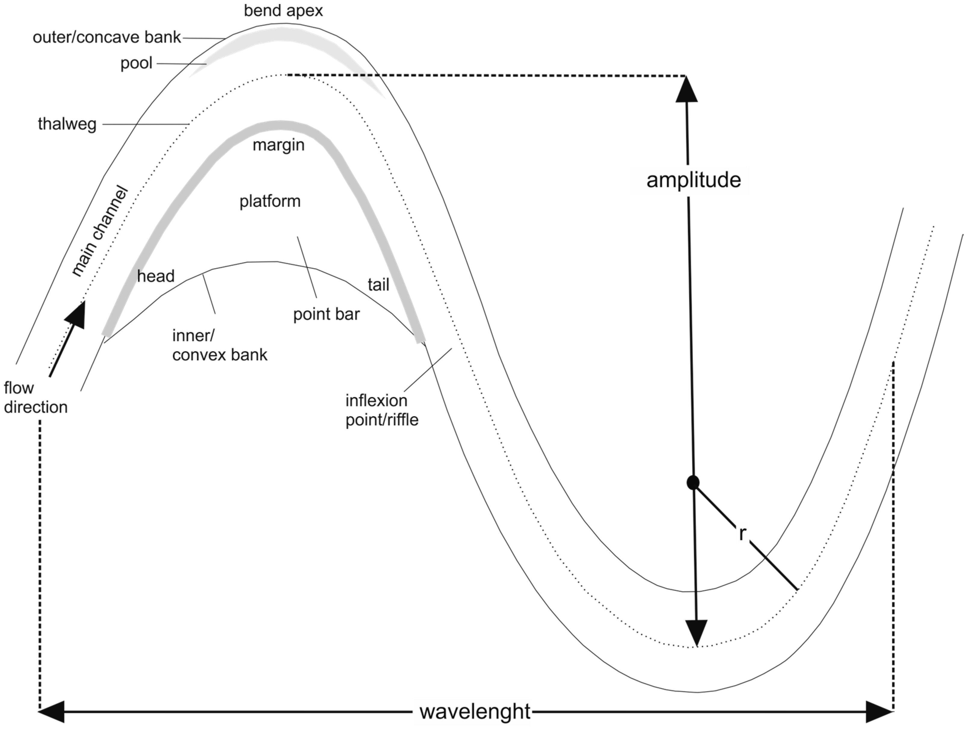
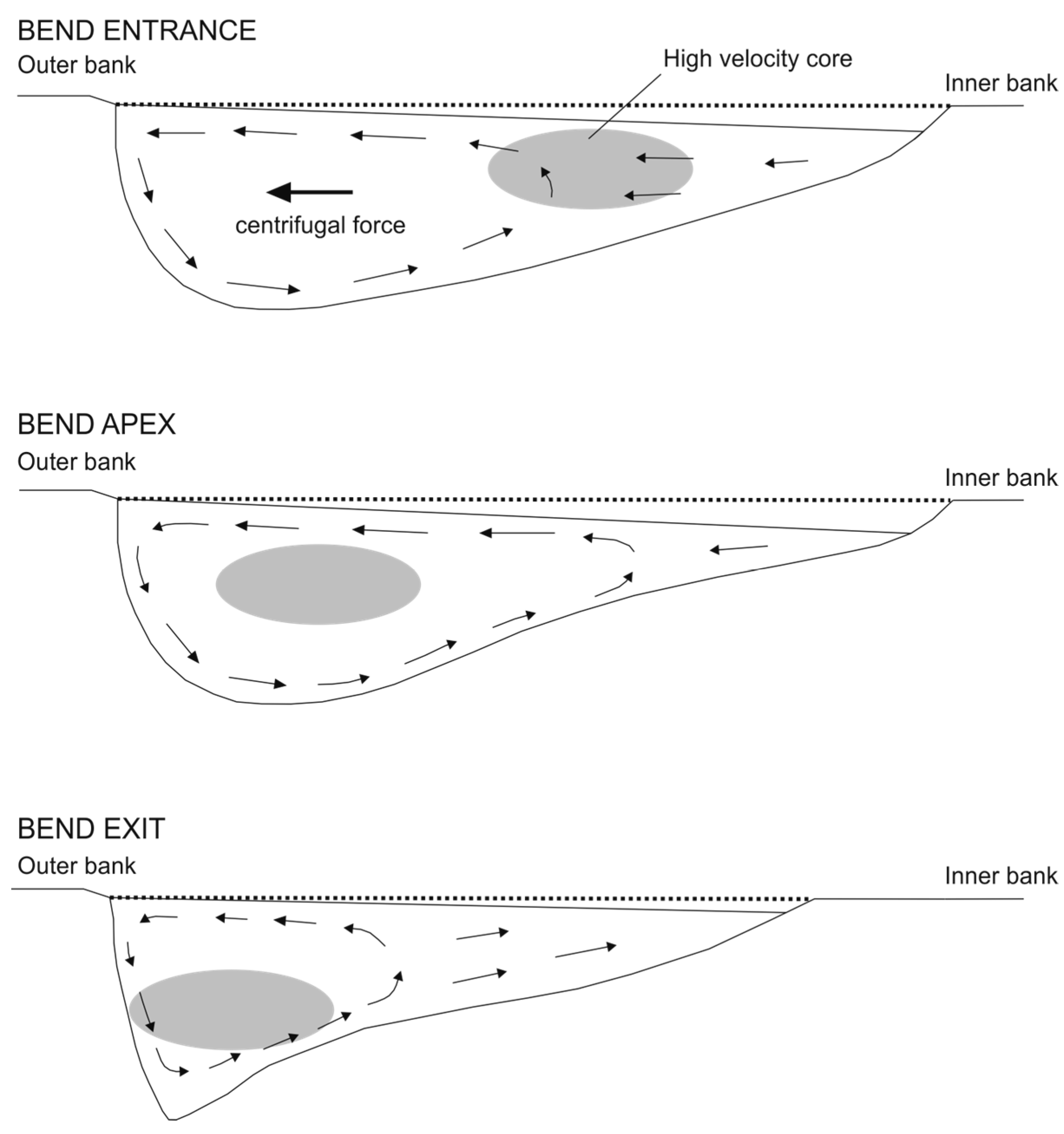
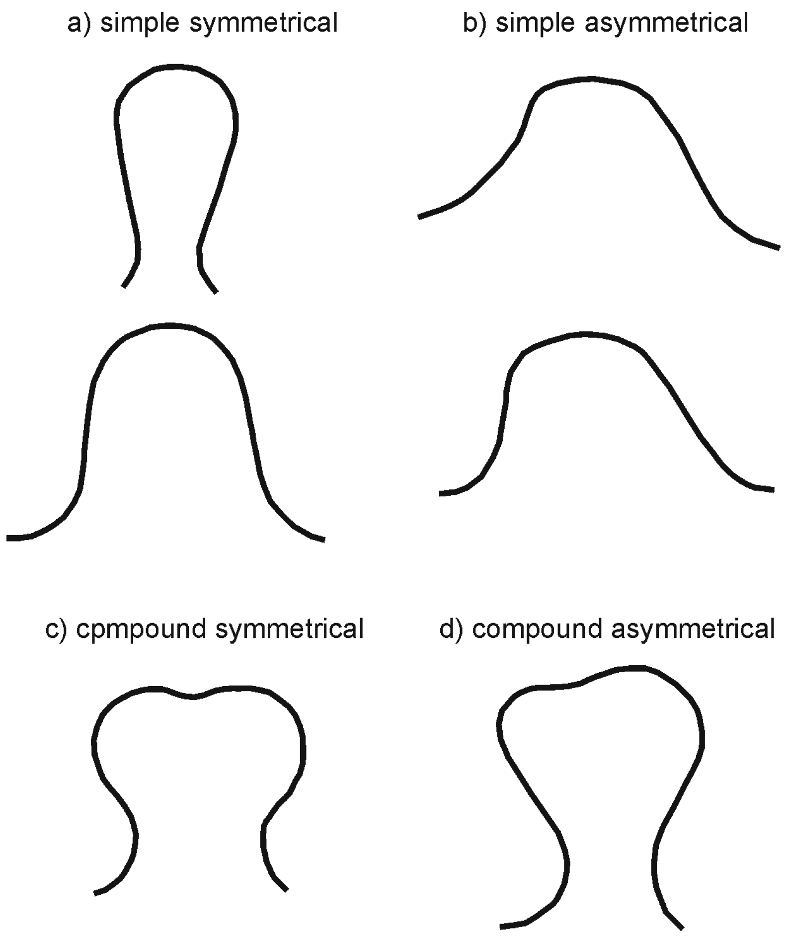
2. Fluvial Geomorphology of Meandering Rivers

In a meandering river, bends with different amplitudes and radii of curvature form a continuous sinuous channel. A meander bend usually consists of a gently sloped point bar attached to the convex side and a deep pool on the steep, concave side [36] (Figure 1). Meandering is initiated as a result of complex interactions between flow, bed sediment, bank material, relief and vegetation. Disturbance of flow in a straight channel, caused for example by an obstacle or uneven sediment size distribution, leads to oscillation of flow and formation of alternate bars. The bed forms, by turn, cause shoaling and divergence of flow, increasing the turbulence and spatial variability of flow velocities in the channel [37]. This enables further bank erosion and bar growth and the formation of curvature along the channel [38,39].

The sinuous channel shape maintains and strengthens the uneven distribution of the flow velocities and sedimentary processes along meander bends. At the meander bend entrance, the high-velocity core (HVC) is situated near the inner bank, shifting gradually towards the outer bank along the bend due to the point bar and the bend curvature [1,2,6,10,41] (Figure 2). The structure of the flow entering the bend depends on the upstream geomorphology of the river and may thus vary depending on the site. The outward flow causes a superelevation at the concave (outer) bank, which enforces a downwards flow along the bank that continues as an inwards near-bed flow and an upwards flow at the inner bank [2,17,36]. This is called secondary circulation [8]. At bends with a steep outer bank, a small cell of reverse rotation may appear near the outer bank [8]. The outward flow may dominate the entire water column at the upstream part of the point bar [2]. With the shift of the HVC towards the outer bank, the maximum stream power and sediment transport also shift from the inner bank towards the outer bank with the distance downstream. The low-flow velocities control the bar tail and, accompanied by a recirculation zone at the inner bank beyond the apex, lead to the deposition of fine material over the point-bar tail [1]. During high discharges, the flow can straighten its way across the point-bar platform, eroding the point bar platform and, in some cases, creating a chute channel on the point bar [1,10,36]. This has been noted to inhibit the growth of sinuosity and thereby the meander evolution [32]. At lower discharges, the HVC shifts towards the outer bank further upstream compared to higher discharges [6]. Therefore, during low discharges, the current over the bar head remains weak, enabling small particles to fill the point-bar margin [36,42]. Furthermore, the processes of an individual bend may also depend on the conditions downstream, because backwater effects from downstream can influence upstream flow conditions [43].

Erosion at the outer bank and point bar accumulation cause gradual increases in bend sinuosity and amplitude, leading finally to a sudden sinuosity decrease called neck cutoff. This is the process of meander evolution. In the conceptual models of meander evolution, the meander bends are classified into four groups, depending on the phase of development: simple symmetric, simple asymmetric, compound symmetric and compound asymmetric [44] (Figure 3). In a simple symmetric bend meander, amplitude and sinuosity increase gradually and the point bar grows laterally towards the outer bank [44,45]. The outer bank’s erosion occurs further upstream, and the asymmetry of the bends increases, forming a compound bend and continuing to a cutoff [46,47]. After the cutoff, the development starts from the beginning.

The sub-bend-scale processes (including erosion at the point-bar head or convex bank beyond the apex and deposition over the point-bar tail) are key factors in the meander evolution, leading the bend from one phase to another. However, even though similar kinds of processes and changes are found in meandering channels independent of soil or environmental characteristics, each river still seems to behave uniquely and unpredictably. The special mechanisms that determine the rate and occasion of these changes and finally control the rivers long-term evolution remain unclear. To gain a deeper understanding of these processes would require higher spatial and temporal resolution of the data [21].

3. ADCP—Principles and Applications

Acoustic Doppler velocimeters (ADV) and ADCPs produce 2D or 3D velocity data over the flow field using the Doppler shift principle. The ADV measures the flow field at an individual point, while the ADCP can measure the flow field and discharge within a water column from a moving platform. An ADCP can also measure the bathymetry simultaneously, so it is especially functional in rivers with rapidly changing discharge conditions. Its clear advantage is that it can be operated in deep-water rivers, in areas inaccessible on foot but also in shallow areas. These features have led to increased use of ADCPs by researchers, and a wide range of studies exploiting the ADCP and dealing with flow structure and turbulence have been published [18,42,48,49,50,51,52], some of them focusing on meandering rivers [25,42,49,52]. In most of these studies, however, the 3D flow distribution have been measured along cross-sections and thus the measurements have not covered the whole bend, facing partly similar problems related to the traditional methods [5,49,52]. Although transect-based ADCP measurements are much more efficient than traditional methods and allow for deep-river investigations, they add limited value to the understanding of riverine processes. They have many of the same disadvantages as traditional methods—namely the fact that most of the river reach is not surveyed, and thus the results are highly dependent on the interpolation analysis of the ADCP transect data. Therefore, recent attempts have been made to map the flow field in high resolution with horizontally continuous ADCP data [33,34,35]. The horizontally continuous approach demonstrated by Flener et al. [33] is applied in this study for the first time to study flow patterns and morphological changes in a meander bend.

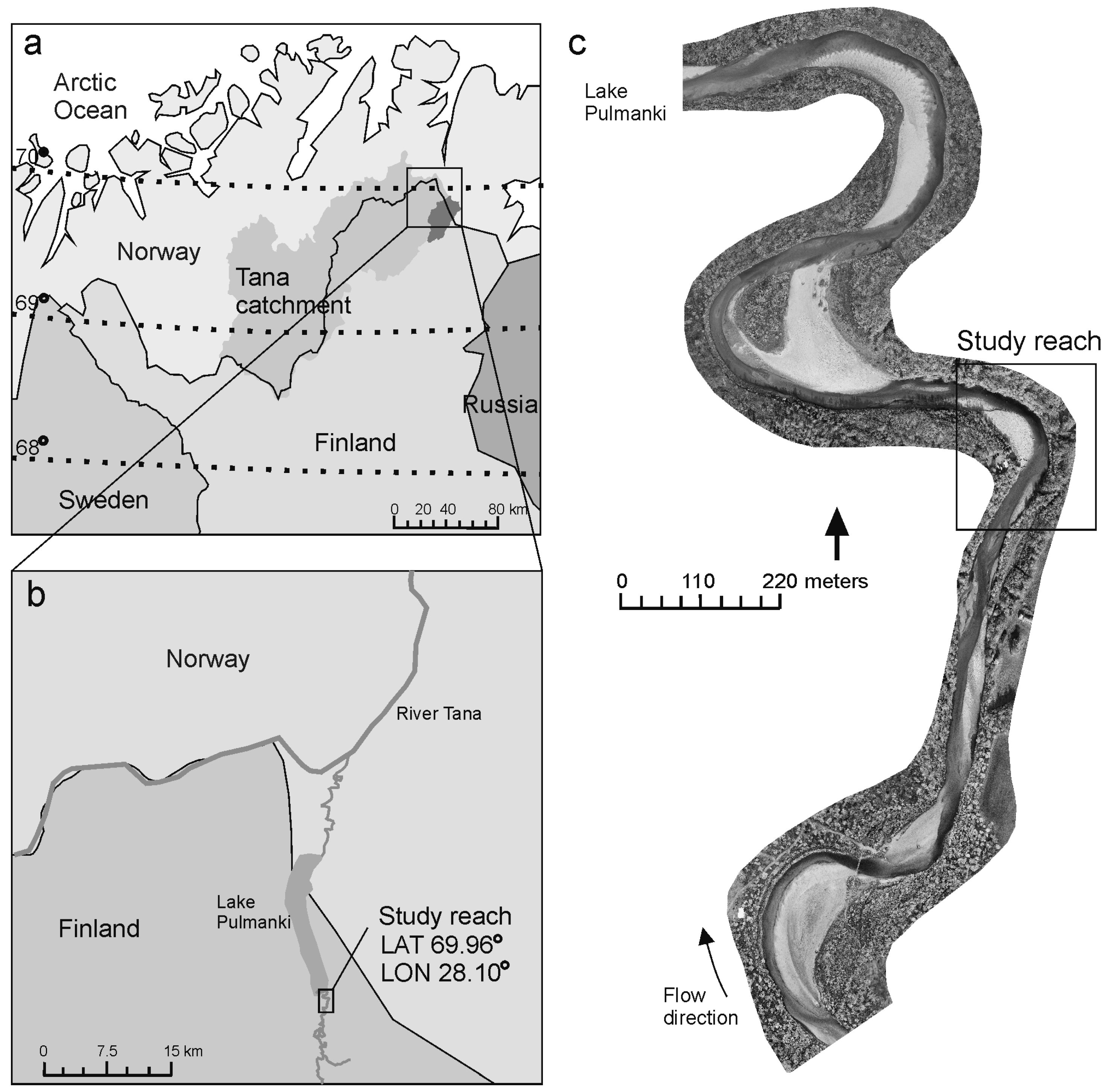
4. Study Area

The study reach is a part of Pulmanki River in Northern Finland (Figure 4). The Pulmanki River is a tributary of the Tana River bordering Finland and Norway. Due to the seasonal weather patterns, a flood event occurs every spring as a result of melting snow. The channel is usually without ice cover from late May until late October. Typical spring flood lasts for one to three weeks during May, and during that time the discharge can exceed more than 10 times the summer low flow (

Table 1. The peak spring flood discharges (in m³·s⁻¹) of the study area during the past eight years. The normal low flow discharge varies between 1.5 and 5 m³·s⁻¹.

Year	Q
2009	42
2010	49
2011	25
2012	39
2013	67
2014	43
2015	30
2016	15

).

The study was carried out in a sandy and highly mobile meander bend, 230 m in length (along the channel centerline) with a gradient of 0.0002. The bend has a sinuosity of 1.5, a radius of curvature at the apex of 110 m, and a width-to-depth ratio of 14. The channel width at the apex varies between 20 and 55 during low-flow and flood conditions, respectively. The outer bank is steep and covered by vegetation. The D₅₀ of the sediment varies mostly between 0.2 and 0.8 mm, the larger sediment being located mostly in the deeper (i.e., main channel) and smaller sediments in the shallower parts (i.e., point bar) of the bend. There is a sandy unvegetated point bar in the inner bend with size of approximately 3000 m². During the spring flood of 2013, the water level was 2 m above that of the summer low flow and the point bar was completely inundated. The spring flood discharge of 2013 was untypically high (Table 1).

The area is well-suited as a test site to investigate fluvial processes and channel changes; hence several fluvio-geomorphological studies have been performed in the same river reach during the last ten years. These studies have shown that vertical changes up to 0.7 m occur annually on the point bars during the spring flood period [42]. According to the previous studies, however, the morphological changes of consecutive years can differ notably from each other, and changes in one bend are not clearly connected to changes in another bend [21,22]. Even though most of the changes on the point bars are related to flood events, as they are not otherwise inundated, such changes also occur during the decreasing limb of the flood—that is, during the periods of decreased stream power. The results of previous studies have also illustrated how the backwater effect may reduce the flow velocities and stream power, especially during the spring flood, by decreasing the discharge and keeping the water surface high, but it has not been analyzed deeply. In this study, we also investigate underwater changes with high temporal resolution for the first time during a flood event.

5. Data Collection and Processing

5.1. Data Collection

During a snowmelt induced spring flood in May 2013, the flow characteristics and bathymetry of the study area were measured each day during a period of nine days (16–24 May) using an ADCP attached to a remotely controlled mini-boat. Both the rising and the descending limbs of the flood were captured. A point density of 0.7–1.1 points/m² was achieved. On 18 May, the ADCP was attached to an inflatable boat because the survey was extended to cover a longer reach. On that day, lower data density (0.2 points/m²) was achieved compared to the rest of the measurement days. The field campaign included water level recoding as well as ADCP measurements from a moving platform with simultaneous VRS-GNSS (Virtual reference system global navigation satellite system) measurements of the ADCP location.

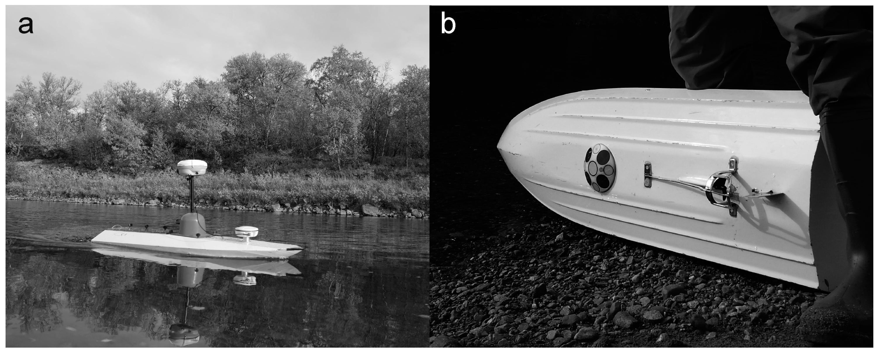
5.1.1. ADCP and VRS-GNSS Measurements

We used an ADCP (Sontek RiverSurveyor M9 [53]) to measure the flow field and bed morphology over the entire bend. The Sontek M9 measures flow velocity and direction with four 3.0-MHz and four 1.0-MHz transducers. The transducers simultaneously emit pulses at multiple frequencies, and a built-in algorithm selects the best return signal for the particular depth and velocity. A vertically oriented echo sounder of 0.5-MHz records the flow depth. According to the manufacturer, the measurement margins of error are 0.25% and 0.1% of the velocity and depth measurements, respectively [54].

For eight of the nine days during the daily measurement campaign, the ADCP sensor was mounted on a custom-designed remotely controlled mini-boat. The mini-boat is 1.43 m long and 0.43 m wide with a draught of 0.17 m. When attached to the boat, the head of the ADCP sensor is 0.06 m below the water surface (Figure 5). The hull of the boat and sensor opening are designed to minimise turbulence and drag. The boat is equipped with a propeller powered by a 24-V motor and can operate in a maximum flow speed of 3 m·s⁻¹. The batteries allow continuous measurement of approximately two hours; we used two sets of batteries to conduct this study. The ADCP was coupled with its own differential GPS (DGPS) and the external VRS-GNSS (Trimble R8) to combine the flow measurements with accurate geographical positions (see [33] for further information).

Before the measurement campaign, the compass of the ADCP was calibrated with reference to the local magnetic field. During the measurements, the boat was controlled to move slower than the average flow speed, with a mean speed of 1 m·s⁻¹. The measurement was performed by moving the boat upstream along a figure-8 shaped track. Thousands of vertical profiles containing 1–75 cells (varying from 0.02 to 0.2 m in height), 3D velocity data, and flow depth were collected during each survey. The final horizontal point density varied between 0.2 and 1.1 points/m² depending on the measurement technique and water level (note the different measurement technique used on 18 May). During the two-hour survey period, the water level did not change significantly. Both the ADCP and VRS-GNSS measurements were recorded with 1Hz frequency.

5.1.2. Recording Water Level

Water surface elevation over the study area was recorded continuously over the measurement campaign using two bottom-mounted water pressure sensors (Solinst Levelogger Gold, Model 3001; accuracy 0.05% [55]) and VRS-GNSS based reference measurements. The pressure sensors were placed on the inner bank at the bend entrance and exit. The measured pressure values were compensated using air pressure data recorded at the study site at the same intervals. In order to tie the water level variation to the geographic coordinate system, the water surface elevation at each of the loggers was measured five times during the field campaign using a VRS-GNSS receiver. A series of consecutive points were measured and averaged in order to achieve as good accuracy as possible. Precision larger than 0.02 m was not accepted. The variation in the water surface elevations during the measurement period was considerably smaller than the vertical precision of the VRS-GNSS. The water pressure sensors records were then converted to water surface elevations based on the VRS-GNSS measurements. Water level surface models were built based on the Levelogger measurements at the bend apex and exit. A water level model was built for each day at the time of the ADCP measurement in order to calculate the bathymetric model with greater accuracy than was possible using the VRS-GNSS (see Section 5.2.2 for further information on bathymetric model building). A very detailed technical description of the data collection and processing is presented by Flener et al. [33].

5.2. Data Processing

5.2.1. Flow Field Data Processing

The accurate x- and y-coordinates for all ADCP survey tracks of the nine-day survey campaign were calculated based on the VRS-GNSS measurements. The VRS-GNSS measurements were first corrected by post-processing the measurements with virtual correction data provided by the Finnish virtual reference station network. This allowed for a baseline positional accuracy of 0.05 m. The VRS-GNSS values were combined with ADCP measurements based on time stamps recorded by both receivers. Then the calculated baselines were exported as a text file containing a UTC time stamp every 0.1 s. Next, the ADCP data were converted to the MATLAB format including the DGPS time stamps. The process of merging the ADCP data with the VRS-GNSS positional data is described in detail by Flener et al. [33].

After compounding the accurate horizontal positions to the ADCP data, spatial flow data sets describing near-bed flow velocities and directions and near-bed stream powers (Equation (1)) were created for each date. The near-bed velocity and stream power values were based on the deepest measured cell (aka. bin) in an ensemble that was not discarded due to side lobe interference, i.e., the reflection of side lobes from the stream bed, which interferes with the reflections from the particles thus contaminating the measurement.

Of the measured data, the mean flow velocity varied between 0.39 and 0.98 m·s⁻²and the maximum flow velocity between 1.39 and 2.4 m·s⁻². The manufacturer reports a precision of 0.25% of the measured velocity value [54]. Thereby maximum flow velocity measurement error caused by the device would have been 0.006 m/s.

The daily near-bed flow data were interpolated using an inverse distance weighting method (IDW) with a grid size of 2 m × 2 m. IDW is reliable within the measurement areas [56] and is the best method for use in an asymmetric measurement network [57]. IDW has been used to interpolate spatial flow velocities [56]; for example, Dinehart and Burau [49] applied it to measure spatial flow velocity changes using ADCP. In order to reduce noise and bring forth the meaningful features in the data, a 3-by-3 filter operation, which smooths the input raster and reduces the significance of anomalous cells, was performed for the interpolated daily morphological change data as well as the near-bed flow velocities.

The near-bed stream power was determined using an equation that quantifies the energy loss of water in the channel bed per unit area [58]:

$$\mathsf{\omega }=\rho \mathrm{g}DSv,$$

(1)

where ρ is the density of water (kg·m⁻³), g is the gravitational acceleration (m·s⁻²), D is the water depth (m), S is the water surface gradient, and v is the near-bed flow velocity (m·s⁻²).

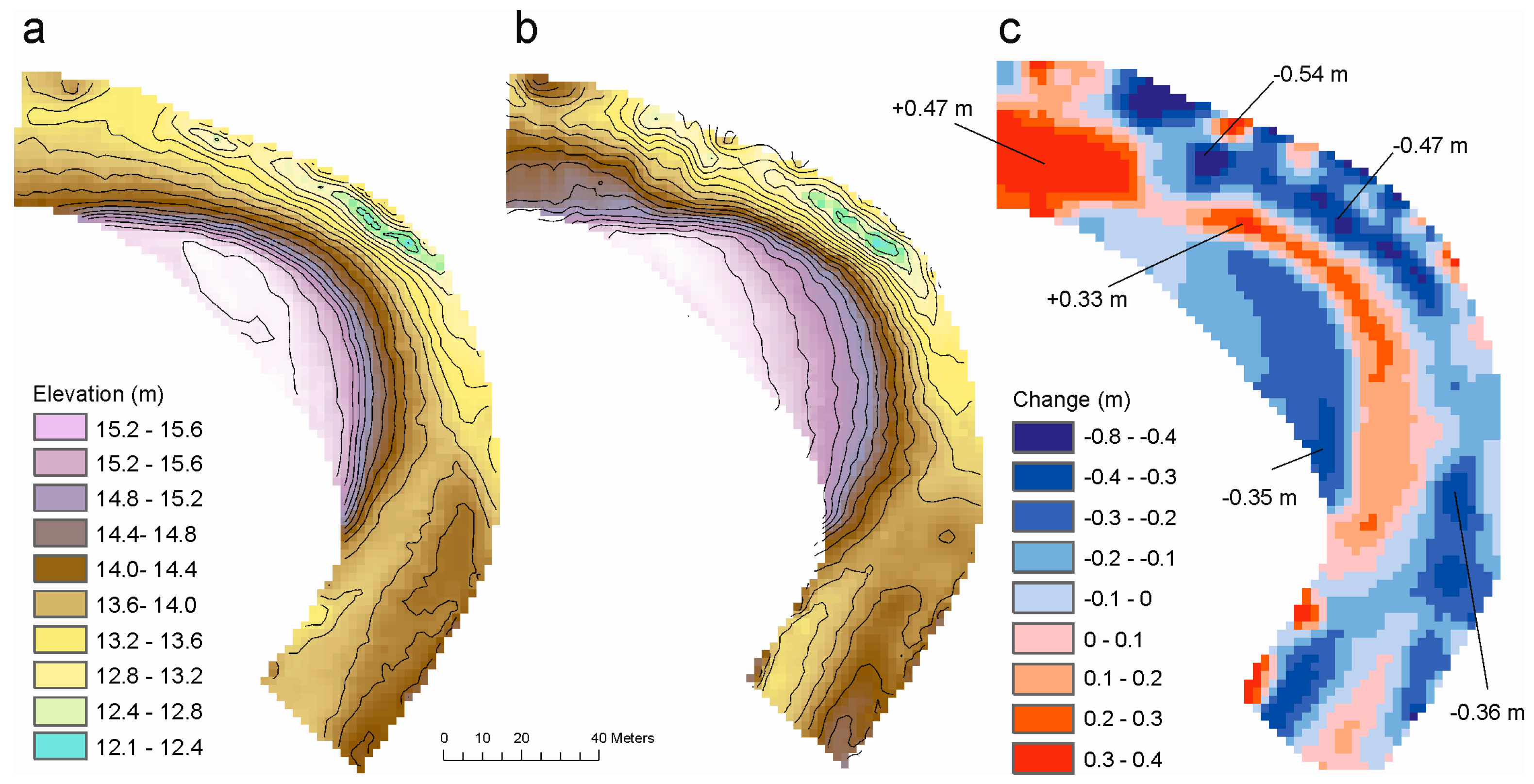
5.2.2. Bathymetric Models and Morphological Change

In order to create bathymetric models as vertically accurate as possible, daily water surface models derived from the water pressure sensor data were created and the z-coordinates of the river bed were calculated by subtracting the ADCP-based depth measurements from the water surface models [24]. The maximum accepted error of the VRS-GNSS measurements of the water surface was 0.02 m. This way, the vertical VRS-GNSS measurement errors in z values, arising mainly from the moving platform measurement, were eliminated, and accurate x-, y-, and z-coordinates of the river bed were derived. The measured mean depth of the data sets varied between 0.93 and 1.58 m and the maximum measured depth between 2.79 and 4.3 m. The manufacturer reports a precision of 1% of the measured depth value. Thereby, the maximum depth measurement error deriving from the device would have been 0.04 m. The errors of the mean depth values have varied between 0.009 and 0.01 m. As the precision of the depth measurement is dependent on the flow depth, measurement error may not have been uniformly distributed across the channel.

Daily digital terrain models (DEMs) of the river bed were calculated by interpolating the resultant x-, y-, and z-point measurements of the river bed, using a 2 m × 2 m grid size with a discretised thin plate spline interpolation method [59]. Morphological changes were derived by calculating the digital elevation models of differences (DoD) by subtracting the digital terrain models of sequential days. Morphological change was calculated for each day as well as the measurement period as a whole. To get an insight on the error propagating from the interpolation of the geometric data, uncertainty of the z-value was calculated for the data of 16 and 17 May by subtracting the interpolated raster value form the original sample value. The average uncertainty (Dz) was calculated for both data sets. Next, the uncertainty propagating form the errors of the individual DEMs ($\partial z$) to the DoD ($\partial z_{DoD}$) was calculated using the following equation:

$$\partial z_{DoD}=\sqrt{{\left(\partial z_a\right)}^2+{\left(\partial z_b\right)}^2}$$

The possible propagated error to the DoD ($\partial z_{DoD}$), deriving from the interpolation of the data was 0.17 m. This is larger than most of the daily changes in our data set. Due to the possible uncertainties of the data, not much attention has been given to the exact magnitudes of morphological changes but rather the spatial distribution of the changes and the morphological activity of each day.

6. Results and Discussion

During the rising stage of the flood, the water level rose 0.9 m (Figure 6), and the discharge almost doubled from 35 to 67 m³·s⁻¹ in a period of less than three days. The water level rose most rapidly between 16 and 20 May. The water level remained high for the rest of the field campaign, but the discharge began to decrease following the flood peak on 19 May. This indicates that the backwater effect forced the water level to stay high but inhibited the flow movement downstream. This dynamic was noted in earlier studies of the same area [42]. As a consequence of the studied flood event, the point-bar platform experienced net erosion and point-bar margins net deposition (Figure 7). Thus, the point bar was growing laterally. The channel thalweg area also experienced net erosion. However, one cannot tell based on Figure 7 whether the erosion occurred continuously throughout the flood or in which phase of the flood the bar-margin deposition occurred. To be able to understand the longer-term meander evolution and its variations in space and time, it is important to gain new insights regarding the continuously ongoing, temporally and spatially small-scale processes in the bend.

Previous studies have indicated that the effect of a flood on point bar morphology may be unexpected in that it does not follow the conceptual model of meander bend evolution [36,42,45]. Kasvi et al. [42] proposed that even though a point-bar head is supposed to be an area of net erosion, it may gain net deposition if the flow and sediment supply conditions are right. Their study also indicated that a point bar may experience both scour and fill during a flood and the eventual morphological change may thus depend on various factors such as the duration of the flood’s descent. However, as their study was based on computational fluid dynamics and spatially intensive but temporally sparse field measurements, they were not able to demonstrate and verify their findings with direct field observations. They stated that temporally intensive field data would be beneficial in studying short-term meander bend evolution.

Our temporally intensive data shows that the high stream power on 17 and 18 May (up to 39 W·m⁻² on 17 May) was accompanied by more active morphological changes (Figure 8, part 1) at the beginning of the flood. Thus, a positive hysteresis effect in sediment transport was observed during this particular spring flood, which was greater than average flooding of the Pulmanki River. The spatial patterns and magnitudes of morphological changes did not, however, follow the distribution of stream power directly (Figure 8). During the days of high stream power in particular, the deep channel area was eroded and point-bar margins gained deposition, and notable outer bank erosion also occurred upstream of the bend apex. This was probably a consequence of the combination of high stream powers and low water levels, which prevented the flow from straightening its way across the point bar. The point bar top experienced minor erosion as soon as it was inundated on 19 May. The near-bed flow was directed slightly towards the outer bank over the point bar, which may have intensified the erosion of the point bar top as the particles may have rolled or slid down the slope of the point bar towards the thalweg [10]. During our nine-day measurement period, the highest part of the point bar was inundated for four days, during which it lost 0.2 m of its height (Figure 9). In addition, the shallowest pool was 0.2 m deeper after the flood due to erosion, which mostly took place during the high stream-power period at the beginning of the flood. Notably lower near-bed stream power values were measured after 19 May: the highest stream power measured on 19 May was 29.7 W·m⁻², and on 20 May it was only 3.1 W·m⁻². This decrease in stream power had an effect on the magnitude of morphological changes: from the 20 May onwards, most morphological changes were less than 0.1 m. The last two measurement days (22 and 23 May) showed low stream-power values (mostly less than 3 W·m⁻²); during those days, minor deposition dominated the inner bank and thalweg areas. The top of the point bar remained low until 22 May when it experienced some deposition and the area become flat and smooth at the elevation of 15.4 m (Figure 9). The deposition during the decreasing discharge was intensified by the backwater effect, which kept the water level high, the point bar inundated, and the flow velocities low (mostly less than 1 m·s⁻¹) even though the discharge decreased.

To see whether there was any clear spatial correlation between the flow and morphology, the correlation between the morphological changes and near bed velocity and stream power was calculated (

Table 2. The Pearson correlation between the morphological change (m) and stream power (W·m⁻²) and near bed velocity (m·s⁻¹) on 18 and 22 May. The analyses were calculated for all data, and also separately for erosional and depositional areas.

	18 May			22 May
	All Data	Deposition	Erosion	All Data	Deposition	Erosion
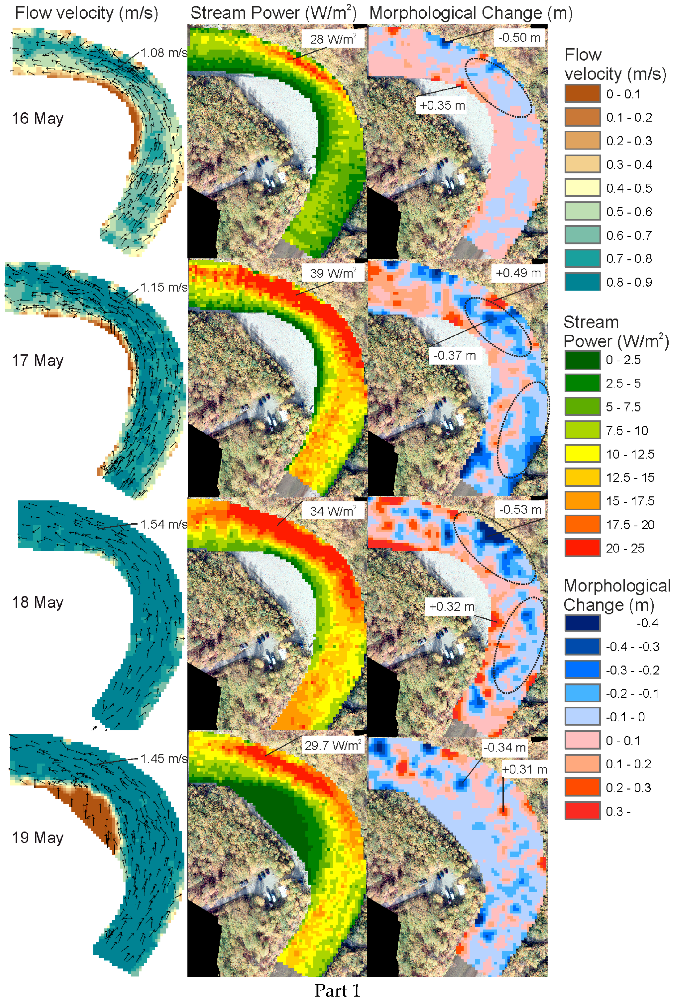
stream power	−0.361 **	−0.122 **	0.206 **	−0.082 **	0.005	−0.114 **
n-b velocity	−0.297 **	−0.145 **	0.243 **	−0.124 **	−0.062 *	−0.134 **

Notes: ** Correlation is significant at the 0.01 level (two-tailed); * Correlation is significant at the 0.05 level (two-tailed).

). Data from 18 and 22 May were applied, as they represented different fluvio-morphological conditions (Figure 5). Overall, the correlations were weak. The correlations between the total morphological change and stream power and near-bed velocity were negative on 18 May (High stream power). This means that the less deposition or more erosion had occurred, the greater the stream power or near bed velocity had been in that location. The strongest correlation (−0.316) was between the morphological changes (both erosion and deposition) and stream power on 18 May. In general, the correlations were stronger within the areas experiencing erosion, than experiencing deposition. Overall correlations were weaker on 22 May than on 18 May. The correlation was almost non-existent within the areas experiencing deposition on 22 May. Noteworthy is that the correlation is significant at 0.01 level in every other calculation, except when morphological changes at deposition areas are analyzed against the stream power and near bed velocity on 22 May. As the stream power was calculated based on the measured flow depth and velocity, the errors propagating from the measurements (see Section 4 for further details) also affect the stream power values.

The current data set confirms the results of earlier studies [21] that suggested that different parts of the point bar can experience erosion and deposition during a flood independent of the net morphological change of the area. In fact, the final net deposition over the point bar seems to be, in this case, partly a result of the backwater effect, which lowered the stream power and thereby enabled the deposition. However, the bar head area, which is normally considered an area of net erosion, gained deposition during the flood peak when the stream power and flow velocities were high. This shows that, even though the studies of Kasvi et al. [42] and McGowen and Garner [36] indicated that bar head deposition is a consequence of moderate- and low-flow stages, it can actually occur even during high flows.

Furthermore, near the outer bank, there was a daily oscillation of notable magnitudes of erosion and deposition (Figure 8). On 20 May, a local deposition of 0.75 m occurred near the outer bank beyond the apex. As the stream power was relatively low (mostly less than 3 W·m⁻²) and just minor morphological changes (<0.1 m, smaller than the errors in our data), occurred otherwise, it can be assumed that the notable outer bank deposition was the consequence of a bank failure. On 21 May, the same area gained net erosion up to 0.63 m. This could indicate that the loose bed material that had collapsed a day earlier was transported downstream. Again, the same area gained net deposition on 22 May and erosion on 23 May, indicating a similar cycle of bank failure and transportation of the eroded material. The same phenomenon was already evident during the more powerful phase of the flood, from 16 to 19 May. Thus, bank erosion was active throughout the flood. The bank area gained net erosion as a consequence of the flood (Figure 4c).

At the inner bank, the point bar was eroding and gaining material independent of the changes in the flow (Figure 8). This shows that other factors, such as sediment supply and possibly initiating vegetation growth, could affect the morphodynamics. Perhaps also the freshly deposited material is transported away more easily compared to the sediment that has stayed in one place longer, a phenomenon that is also connected to vegetation and point bar flood-plain transition [32]. The inner and outer bank processes were balanced such that the outer bank eroded while the point bar was growing laterally.

According to our data, the morphological processes were more active near the outer bank compared to the inner bank (Figure 8). However, it is difficult to determine whether the development was driven by the erosion of the outer bank or deposition of the inner bank. At the beginning of the flood, during high stream powers, the inner and outer bank processes seemed to occur simultaneously (Figure 8). However, at the end of the measurement period, the inner bank morphological changes were mostly minor, while the outer bank was evolving more actively. This could indicate that the outer bank erosion was the driving force of the meander migration in this case, as it occurred despite the lack of inner bend push. This is consistent with earlier studies by Hooke [28], Gautier et al. [29], Eke [30] and Van de Lageweg et al. [31] and thus slightly contradictory to the recent study of Schuurman et al. [32], who stated that “inner bank push” is required for the development of high-sinuosity meanders with neck cutoffs. However, they also noted that high outer-bank erodibility may diminish the necessity of inner bank push, which could be the case in our study reach where the outer bank was eroding. Compared to the results of the earlier studies, the consequences of the backwater effect on the morphodynamics are not easily distinguishable from other types of rivers behavior.

Based on our data set of only one year and one meander bend, it is difficult to draw conclusions about the effects of these processes on longer-term meander evolution. The investigated bend is a simple symmetric bend that was growing in amplitude, and the point bar showed lateral growth towards the outer bank. Simultaneously, the asymmetry of the bend was increasing, as the outer bank was also eroding upstream of the apex. This is typical behavior of a simple symmetric bend transforming towards an asymmetric shape [44,45]. However, our data showed that the changes were dependent on the stream power present in the inundated area (i.e., water level), and that the time period of low stream power was dominated by deposition, although the outer bank was still eroding. A long duration of high stream power could thereby hinder point-bar growth. Thus, in such a case the meander evolution would be driven by inner bank push, which would also hinder the overall meander evolution. On the other hand, the backwater effect during the flood could actually advance the bend development by allowing sedimentation on the point bar, as noted by Lotsari et al. [22]. This is an important finding, especially regarding rivers with strong backwater effects during flood events. The effects of flood events on river evolution should get more attention in future studies, as flood regimes are expected to change along with the changing climate, especially in high altitudes and latitudes [60].

Our study approach provided a novel way to investigate the spatial and temporal patterns of the fluvial processes in a natural riverine environment. The mini-boat approach fitted very well in a river with both deep and shallow areas. For example, even though side-scanning sonar enables high spatial resolution, it requires more flow depth [61,62]. There have also been attempts to develop new methods that would enhance the bathymetric data resolution and density by using optical methods [63,64,65]. Optical methods could allow for higher accuracy bathymetric models, provided that the water is clear enough, but they do not measure the flow characteristics simultaneously. In the future, the possibilities provided by modern research approaches and their combinations should be fully exploited by fluvial geomorphologists to solve the remaining research questions.

7. Conclusions

This study demonstrated the application of a remotely controlled mini-boat equipped with an ADCP device and high accuracy GNSS to investigate short-term and small-scale flow and sediment dynamics in a meander bend during a flood. The ADCP measured the flow characteristics (e.g., stream power, flow velocities and directions) and the river bed elevation simultaneously. To our knowledge, this is the first study to use daily measurements of flow and morphology with high spatial resolution (0.2–1.1 points/m²) to investigate this subject. The methodological approach allowed for dense data collection during a period (approximately 2 h) in which the flow conditions did not change notably, and the remotely controlled boat platform allowed us to take measurements over shallow areas without disturbing the flow field and river bed. The spatially and temporally intensive data set of this study showed that erosion dominated during periods of high discharge and stream power and deposition dominated during low discharge and stream power, both in the channel and over the point bar. However, both erosion and deposition occurred throughout the flood. The magnitudes of the morphological changes were also more notable during periods of high stream power compared to low-discharge periods. Thus, the flood duration and the rate of discharge increase and decrease seems to play key roles in determining the total morphological changes and thus also the longer-term river evolution. A long duration of high stream power may have a hindering effect on point-bar growth. During the measurement period of one flood, the inner bank and outer bank movements were more or less balanced and no clear indications of inner bend push or outer bank pull were observed. However, a daily oscillation of notable erosion and deposition was evident near the outer bank throughout the measurement period. This was interpreted to be a consequence of bank failure and transportation of the eroded loose-bed material downstream. Furthermore, the backwater effect may inhibit meander evolution by decreasing the temporal extension of high stream powers during a flood. On the other hand, it may allow point-bar growth by extending the inundation period and thereby advancing the meander evolution. Future research should study the effects of vegetation success and bar-floodplain conversion on the flood-induced morphological changes of meanders and how these are related to outer bank erosion in a natural channel, using high resolution data over multiple years. Short-term changes can be very spatially fragmented and thus reflect poorly the longer-term changes, as bar and dune dynamics and sediment supply play more important roles. On the other hand, these short-term processes might give new insights into the various factors influencing longer-term developments. Therefore, it would be necessary to study several meander bends and different flow events to better understand how these processes affect long-term meander evolution. The methodological approach demonstrated in this study is feasible for use in the further studies.

References

- Bridge, J.S.; Jarvis, J. Flow and sedimentary processes in the meandering river South Esk, Glen Clova, Scotland. Earth Surf. Process. 1976, 1, 303–336. [Google Scholar] [CrossRef]
- Dietrich, W.E.; Smith, J.D. Influence of the point bar on flow through curved channels. Water Resour. Res. 1983, 19, 1173–1192. [Google Scholar] [CrossRef]
- Ferguson, R.I.; Ashwoth, P.J. Spatial patterns of bedload transport and channel change in braided and near braided rivers. In Dynamics of Gravel-Bed Rivers; Billi, P., Hey, R.D., Thorne, C.R., Tacconi, P., Eds.; Wiley: Chichester, UK, 1993. [Google Scholar]
- Warburton, J.; Davies, T.R.; Mandl, M. A meso-scale field investigation of channel change and floodplain characteristics in an upland braided gravel-bed river, New Zealand. In Braided Rivers; Best, J.L., Bristow, C.S., Eds.; Geological Society Special Publication: London, UK, 1993. [Google Scholar]
- Frothingham, K.M.; Rhoads, B.L. Three-dimensional flow structure and channel change in an asymmetrical compound meander loop, Embarras River, Illinois. Earth Surf. Process. Landf. 2003, 28, 625–644. [Google Scholar] [CrossRef]
- Hooke, R.L.B. Distribution of Sediment Transport and Shear Stress in a Meander Bend. J. Geol. 1975, 83, 543–565. [Google Scholar] [CrossRef]
- Jackson, R.G. Velocity–bed-form–texture patterns of meander bends in the lower Wabash River of Illinois and Indiana. Geol. Soc. Am. Bull. 1975, 86, 1511–1522. [Google Scholar] [CrossRef]
- Bathurst, J.C.; Hey, R.D.; Thorne, C.R. Secondary flow and shear stress at river bends. J. Hydraul. Div. 1979, 105, 1277–1295. [Google Scholar]
- Bluck, B.J. Texture of gravel bars in braided stream. In Gravel-Bed Rivers; Hey, R.D., Bathurst, J.C., Thorne, C.R., Eds.; Wiley: Chichester, UK, 1982. [Google Scholar]
- Dietrich, W.E.; Smith, J.D. Bed Load Transport in a River Meander. Water Resour. Res. 1984, 20, 1355–1380. [Google Scholar] [CrossRef]
- Thompson, A. Secondary flows and the pool-riffle unit: A case study of the processes of meander development. Earth Surf. Process. Landf. 1986, 11, 631–641. [Google Scholar] [CrossRef]
- Lane, S.N.; Richards, K.S.; Chandler, J.H. Developments in monitoring and modelling small-scale river bed topography. Earth Surf. Process. Landf. 1994, 19, 349–368. [Google Scholar] [CrossRef]
- Heritage, G.L.; Fuller, I.C.; Charlton, M.E.; Brewer, P.A.; Passmore, D.P. CDW photogrammetry of low relief fluvial features: Accuracy and implications for reach-scale sediment budgeting. Earth Surf. Process. Landf. 1998, 23, 1219–1233. [Google Scholar] [CrossRef]
- Brasington, J.; Rumsby, B.T.; McVey, R.A. Monitoring and modelling morphological change in a braided gravel-bed river using high resolution GPS-based survey. Earth Surf. Process. Landf. 2000, 25, 973–990. [Google Scholar] [CrossRef]
- Fuller, I.C.; Large, A.R.G.; Milan, D.J. Quantifying channel development and sediment transfer following chute cutoff in a wandering gravel-bed river. Geomorphology 2003, 54, 307–323. [Google Scholar] [CrossRef]
- Heritage, G.; Hetherington, D. Towards a protocol for laser scanning in fluvial geomorphology. Earth Surf. Process. Landf. 2007, 32, 66–74. [Google Scholar] [CrossRef]
- Bridge, J.S.; Jarvis, J. The dynamics of a river bend: A study in flow and sedimentary processes. Sedimentology 1982, 29, 499–541. [Google Scholar] [CrossRef]
- Guerrero, M.; Lamberti, A. Flow Field and Morphology Mapping Using ADCP and Multibeam Techniques: Survey in the Po River. J. Hydraul. Eng. 2011, 137, 1576–1587. [Google Scholar] [CrossRef]
- Brasington, J.; Langham, J.; Rumsby, B. Methodological sensitivity of morphometric estimates of coarse fluvial sediment transport. Geomorphology 2003, 53, 299–316. [Google Scholar] [CrossRef]
- Westaway, R.M.; Lane, S.N.; Hicks, D.M. Remote survey of large-scale braided, gravel-bed rivers using digital photogrammetry and image analysis. Int. J. Remote Sens. 2003, 24, 795–815. [Google Scholar] [CrossRef]
- Kasvi, E.; Vaaja, M.; Kaartinen, H.; Kukko, A.; Jaakkola, A.; Flener, C.; Hyyppä, H.; Hyyppä, J.; Alho, P. Sub-bend scale flow–sediment interaction of meander bends—A combined approach of field observations, close-range remote sensing and computational modelling. Geomorphology 2015, 238, 119–134. [Google Scholar] [CrossRef]
- Lotsari, E.; Vaaja, M.; Flener, C.; Kaartinen, H.; Kukko, A.; Kasvi, E.; Hyyppä, H.; Hyyppä, J.; Alho, P. Annual bank and point bar morphodynamics of a meandering river determined by high-accuracy multitemporal laser scanning and flow data. Water Resour. Res. 2014, 50, 5532–5559. [Google Scholar] [CrossRef]
- Darby, S.E.; Alabyan, A.M.; Van de Wiel, M.J. Numerical simulation of bank erosion and channel migration in meandering rivers: Simulating bank erosion in menadering rivers. Water Resour. Res. 2002, 38. [Google Scholar] [CrossRef]
- Ottevanger, W.; Blanckaert, K.; Uijttewaal, W.S.J. Processes governing the flow redistribution in sharp river bends. Geomorphology 2012, 163–164, 45–55. [Google Scholar] [CrossRef]
- Engel, F.L.; Rhoads, B.L. Interaction among mean flow, turbulence, bed morphology, bank failures and channel planform in an evolving compound meander loop. Geomorphology 2012, 163–164, 70–83. [Google Scholar] [CrossRef]
- Hooke, J.M.; Yorke, L. Rates, distributions and mechanisms of change in meander morphology over decadal timescales, River Dane, UK. Earth Surf. Process. Landf. 2010, 35, 1601–1614. [Google Scholar] [CrossRef]
- Hackney, C.; Best, J.; Leyland, J.; Darby, S.E.; Parsons, D.; Aalto, R.; Nicholas, A. Modulation of outer bank erosion by slump blocks: Disentangling the protective and destructive role of failed material on the three-dimensional flow structure: Impact of slump blocks on 3-D flow field. Geophys. Res. Lett. 2015, 42, 10663–10670. [Google Scholar] [CrossRef]
- Hooke, J.M. Spatial variability, mechanisms and propagation of change in an active meandering river. Geomorphology 2007, 84, 277–296. [Google Scholar] [CrossRef]
- Gautier, E.; Brunstein, D.; Vauchel, P.; Jouanneau, J.-M.; Roulet, M.; Garcia, C.; Guyot, J.-L.; Castro, M. Channel and floodplain sediment dynamics in a reach of the tropical meandering Rio Beni (Bolivian Amazonia). Earth Surf. Process. Landf. 2010, 35, 1838–1853. [Google Scholar] [CrossRef]
- Eke, E. Numerical Modeling of River Migration Incorporating Erosional and Depositional Bank Processes. Ph.D. Thesis, University of Illinois, Chicago, IL, USA, 2013. [Google Scholar]
- Van de Lageweg, W.I.; van Dijk, W.M.; Baar, A.W.; Rutten, J.; Kleinhans, M.G. Bank pull or bar push: What drives scroll-bar formation in meandering rivers? Geology 2014, 42, 319–322. [Google Scholar] [CrossRef]
- Schuurman, F.; Shimizu, Y.; Iwasaki, T.; Kleinhans, M.G. Dynamic meandering in response to upstream perturbations and floodplain formation. Geomorphology 2016, 253, 94–109. [Google Scholar] [CrossRef]
- Flener, C.; Wang, Y.; Laamanen, L.; Kasvi, E.; Vesakoski, J.-M.; Alho, P. Empirical Modeling of Spatial 3D Flow Characteristics Using a Remote-Controlled ADCP System: Monitoring a Spring Flood. Water 2015, 7, 217–247. [Google Scholar] [CrossRef]
- Williams, R.D.; Brasington, J.; Hicks, M.; Measures, R.; Rennie, C.D.; Vericat, D. Hydraulic validation of two-dimensional simulations of braided river flow with spatially continuous aDcp data: Two-dimensional simulation of braided river flow. Water Resour. Res. 2013, 49, 5183–5205. [Google Scholar] [CrossRef]
- Williams, R.D.; Rennie, C.D.; Brasington, J.; Hicks, D.M.; Vericat, D. Linking the spatial distribution of bed load transport to morphological change during high-flow events in a shallow braided river: Spatially distributed bedload transport. J. Geophys. Res. Earth Surf. 2015, 120, 604–622. [Google Scholar] [CrossRef]
- Mcgowen, J.H.; Garner, L.E. Physiographic features and stratification types of coarse-grained pointbars: Modern and ancient examples. Sedimentology 1970, 14, 77–111. [Google Scholar] [CrossRef]
- Rhoads, B.L.; Welford, M.R. Initiation of river meandering. Prog. Phys. Geogr. 1991, 15, 127–156. [Google Scholar] [CrossRef]
- Ackers, P.; Charlton, F.G. Meander geometry arising from varying flows. J. Hydrol. 1970, 11, 230–252. [Google Scholar] [CrossRef]
- Schumm, S.A.; Khan, H.R. Experimental Study of Channel Patterns. Geol. Soc. Am. Bull. 1972, 83, 1755. [Google Scholar] [CrossRef]
- Kasvi, E. Fluvio-Morphological Processes of Meander Bends—Combining Conventional Field Measurements, Close-Range Remote Sensing and Computational Modelling. Ph.D. Thesis, University of Turku, Turku, Finland, 2015. [Google Scholar]
- Dietrich, W.E.; Smith, J.D.; Dunne, T. Flow and Sediment Transport in a Sand Bedded Meander. J. Geol. 1979, 87, 305–315. [Google Scholar] [CrossRef]
- Kasvi, E.; Vaaja, M.; Alho, P.; Hyyppä, H.; Hyyppä, J.; Kaartinen, H.; Kukko, A. Morphological changes on meander point bars associated with flow structure at different discharges. Earth Surf. Process. Landf. 2013, 38, 577–590. [Google Scholar] [CrossRef]
- Smith, J.D.; Mclean, S.R. A Model for Flow in Meandering Streams. Water Resour. Res. 1984, 20, 1301–1315. [Google Scholar] [CrossRef]
- Brice, J.C. Evolution of Meander Loops. Geol. Soc. Am. Bull. 1974, 85, 581. [Google Scholar] [CrossRef]
- Hickin, E.J. The development of meanders in natural river-channels. Am. J. Sci. 1974, 274, 414–442. [Google Scholar] [CrossRef]
- Hooke, J.M. River channel adjustment to meander cutoffs on the River Bollin and River Dane, northwest England. Geomorphology 1995, 14, 235–253. [Google Scholar] [CrossRef]
- Parker, G.; Andrews, E.D. On the time development of meander bends. J. Fluid Mech. 1986, 162, 139–156. [Google Scholar] [CrossRef]
- Claude, N.; Rodrigues, S.; Bustillo, V.; Bréhéret, J.-G.; Tassi, P.; Jugé, P. Interactions between flow structure and morphodynamic of bars in a channel expansion/contraction, Loire River, France. Water Resour. Res. 2014, 50, 2850–2873. [Google Scholar] [CrossRef]
- Dinehart, R.L.; Burau, J.R. Repeated surveys by acoustic Doppler current profiler for flow and sediment dynamics in a tidal river. J. Hydrol. 2005, 314, 1–21. [Google Scholar] [CrossRef]
- Nystrom, E.A.; Rehmann, C.R.; Oberg, K.A. Evaluation of Mean Velocity and Turbulence Measurements with ADCPs. J. Hydraul. Eng. 2007, 133, 1310–1318. [Google Scholar] [CrossRef]
- Rennie, C.D.; Church, M. Mapping spatial distributions and uncertainty of water and sediment flux in a large gravel bed river reach using an acoustic Doppler current profiler. J. Geophys. Res. 2010, 115, F03035. [Google Scholar] [CrossRef]
- Riley, J.D.; Rhoads, B.L. Flow structure and channel morphology at a natural confluent meander bend. Geomorphology 2012, 163–164, 84–98. [Google Scholar] [CrossRef]
- Sontek. Sontek Riversurveyor M9. Available online: http://www.xylemanalytics.co.uk/media/pdfs/riversurveyor-s5-m9-eng-%282013-07-26%29r.pdf (accessed on 10 February 2017).
- Sontek. RiverSurveyor S5/M9 System Manual, Firmware Version 3.50; SonTek, a Xylem Brand: San Diego, CA, USA, 2013. [Google Scholar]
- Solinst. Solinst Levelogger Gold. Available online: https://www.solinst.com/products/dataloggers-and-telemetry/3001-levelogger-series/operating-instructions/user-guide/1-introduction/1-1-7-levelogger-gold.php (accessed on 8 February 2017).
- Richtman, C. A GIS Method for Determining Volumetric Flow in a Riverine Channel; Saint Mary’s University of Minnesota Central Services Press: Winona, MN, USA, 2006. [Google Scholar]
- David, L.; Esnault, A.; Calluaud, D. Comparison of interpolation techniques for 2D and 3D velocimetry. In Proceedings of the 11th International Symposium on Applications of Laser Techniques to Fluid Mechanics, Lisboa, Portugal, 8–11 July 2002.
- Bull, W.B. Threshold of critical power in streams. Geol. Soc. Am. Bull. 1979, 90, 453–464. [Google Scholar] [CrossRef]
- Wahba, G. Spline Models for Observational Data; Society for Industrial and Applied Mathematics: Philadelphia, PA, USA, 1990. [Google Scholar]
- Veijalainen, N.; Lotsari, E.; Alho, P.; Vehviläinen, B.; Käyhkö, J. National scale assessment of climate change impacts on flooding in Finland. J. Hydrol. 2010, 391, 333–350. [Google Scholar] [CrossRef]
- Parsons, D.R.; Best, J.L.; Orfeo, O.; Hardy, R.J.; Kostaschuk, R.; Lane, S.N. Morphology and flow fields of three-dimensional dunes, Rio Paraná, Argentina: Results from simultaneous multibeam echo sounding and acoustic Doppler current profiling. J. Geophys. Res. Earth Surf. 2005, 110. [Google Scholar] [CrossRef]
- Kaeser, A.J.; Litts, T.L.; Tracy, T.W. Using low-cost side-scan sonar for benthic mapping throughout the lower Flint River, Georgia, USA: Low-cost sonar benthic mapping in rivers. River Res. Appl. 2013, 29, 634–644. [Google Scholar] [CrossRef]
- Legleiter, C.J. Remote measurement of river morphology via fusion of LiDAR topography and spectrally based bathymetry. Earth Surf. Process. Landf. 2012, 37, 499–518. [Google Scholar] [CrossRef]
- Flener, C.; Lotsari, E.; Alho, P.; Käyhkö, J. Comparison of empirical and theoretical remote sensing based bathymetry models in river environments. River Res. Appl. 2012, 28, 118–133. [Google Scholar] [CrossRef]
- Williams, R.D.; Brasington, J.; Vericat, D.; Hicks, D.M. Hyperscale terrain modelling of braided rivers: Fusing mobile terrestrial laser scanning and optical bathymetric mapping: Hyperscale terrain modelling of braided rivers. Earth Surf. Process. Landf. 2014, 39, 167–183. [Google Scholar] [CrossRef]