1. Introduction
Following the conclusion of the UN’s Millennium Development Goals in 2015, it was estimated that over 2 billion people had gained access to an improved water source. However, current water resources distribution still highlights water stress and scarcity throughout Africa and Asia, with half of the remaining 700 million people without access to an improved water source located within sub-Saharan Africa [
1]. Therefore, the UN’s 2030 Agenda for Sustainable Development dedicated one of the seventeen Sustainable Development Goals (SDGs) to ensuring
equitable availability of water, integrating water resource management, and encouraging more sustainable withdrawals and supply.
Within sub-Saharan Africa, economic and social growth are both reliant upon the sustainable management of water resources [
2]. However, current water resource management failures and inadequacies can be largely linked to inadequate assessment of water resources [
3]. Unfortunately, the quantification of water resources is both complex and costly, especially within basins that cross socio-political and economic boundaries. Although all inputs into hydrologic models introduce uncertainty, the accurate quantification and spatial distribution of precipitation over a watershed is especially critical for hydrologic estimates of runoff, and, consequently, streamflow [
4,
5]. Unfortunately, over the past few decades, the quantity of rainfall gauge station data in Africa has been drastically declining. In the early 1980s, there were 2400 stations providing rainfall data to public data streams including the Global Historical Climate Network (GHCN) and Global Summary of the Day (GSOD). However, the number of stations declined to 500 by 2010 [
6].
Basins can be considered poorly gauged based on the quantity, spatial distribution, and quality of precipitation data. A low quantity and spatial distribution of rainfall gauge stations can cause overgeneralization and inaccurate quantification of water availability while unreliable or incomplete datasets can be unable to or incorrectly identify seasonal or larger range temporal patterns. In place of high density in situ rainfall gauge stations, hydrologists now have access to precipitation estimates derived from climate reanalysis and remote sensing instruments. Although these datasets may not be exact substitutes to direct measurements, they are often more cost effective, timely, and reliable, thus allowing for seasonal, temporal, and spatial patterns in rainfall to be observed and incorporated into hydrologic models.
In a study performed in Vietnam, the use of several gridded climate reanalysis and remotely-sensed precipitation datasets resulted in comparable model performance of simulating discharge to the use of in situ station data [
7]. In addition, in basins upstream of the Three Gorges Reservoir in China, Yang et al. [
8] compared precipitation datasets derived from land-surface models, reanalysis datasets, and climatology models with in situ station data. They discovered that, in a relatively flat basin, gridded precipitation datasets estimated runoff better than the in situ station data within the SWAT model. Over the last decade, several additional studies [
9,
10,
11] positively reviewed the efficacy of the use of satellite-derived products within hydrologic models, but there was unanimous consensus that continued studies are necessary. Moreover, remote-sensing based or land-surface model precipitation estimates do not consistently outperform in situ data [
12,
13,
14]. Thus, even when creating hydrologic models in poorly gauged regions, it is important to determine whether or not replacing in situ data with precipitation estimation is appropriate.
The purpose of this study was twofold. First, we tested the ease/applicability of the conversion and implementation of the CHIRPS dataset, a gridded satellite-derived precipitation dataset, into a standard hydrologic model. Second, we tested the relative performance of gridded climate reanalysis and satellite-derived precipitation datasets to in situ station precipitation data at estimating streamflow in a data-scarce region in eastern Africa.
2. Study Area
The study was carried out in the Lake Victoria Basin (LVB) (sub-Saharan Africa), which is a vital shared water resource for five different countries. However, because the five nations have differing political and environmental agendas, it has been difficult to monitor and implement water resource management strategies within the LVB, especially without consistent and accurate quantification of resources. Consequently, the basin is experiencing watershed degradation and declines in water quality and quantity [
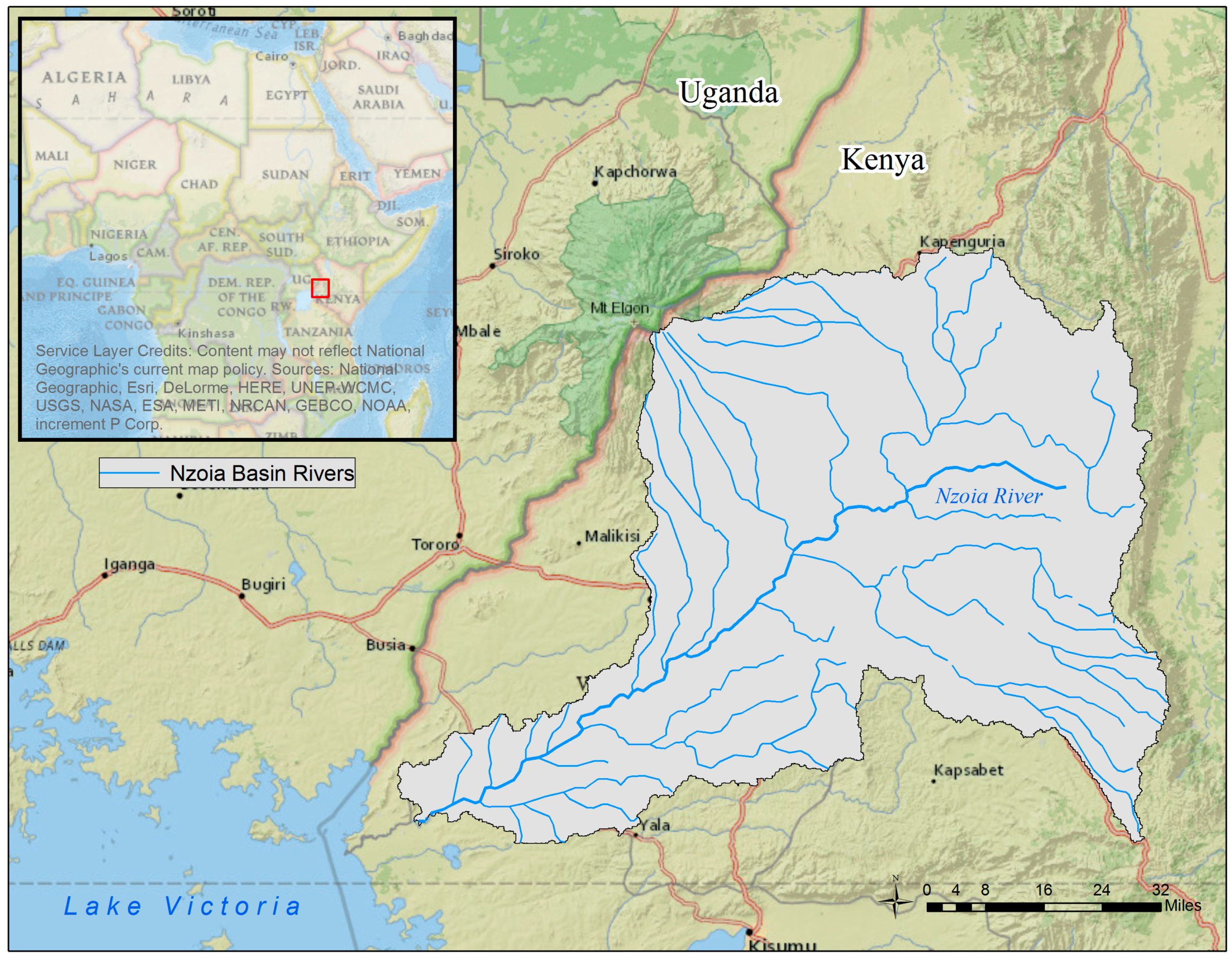
15]. One of the largest tributary contributors to lake inflow [
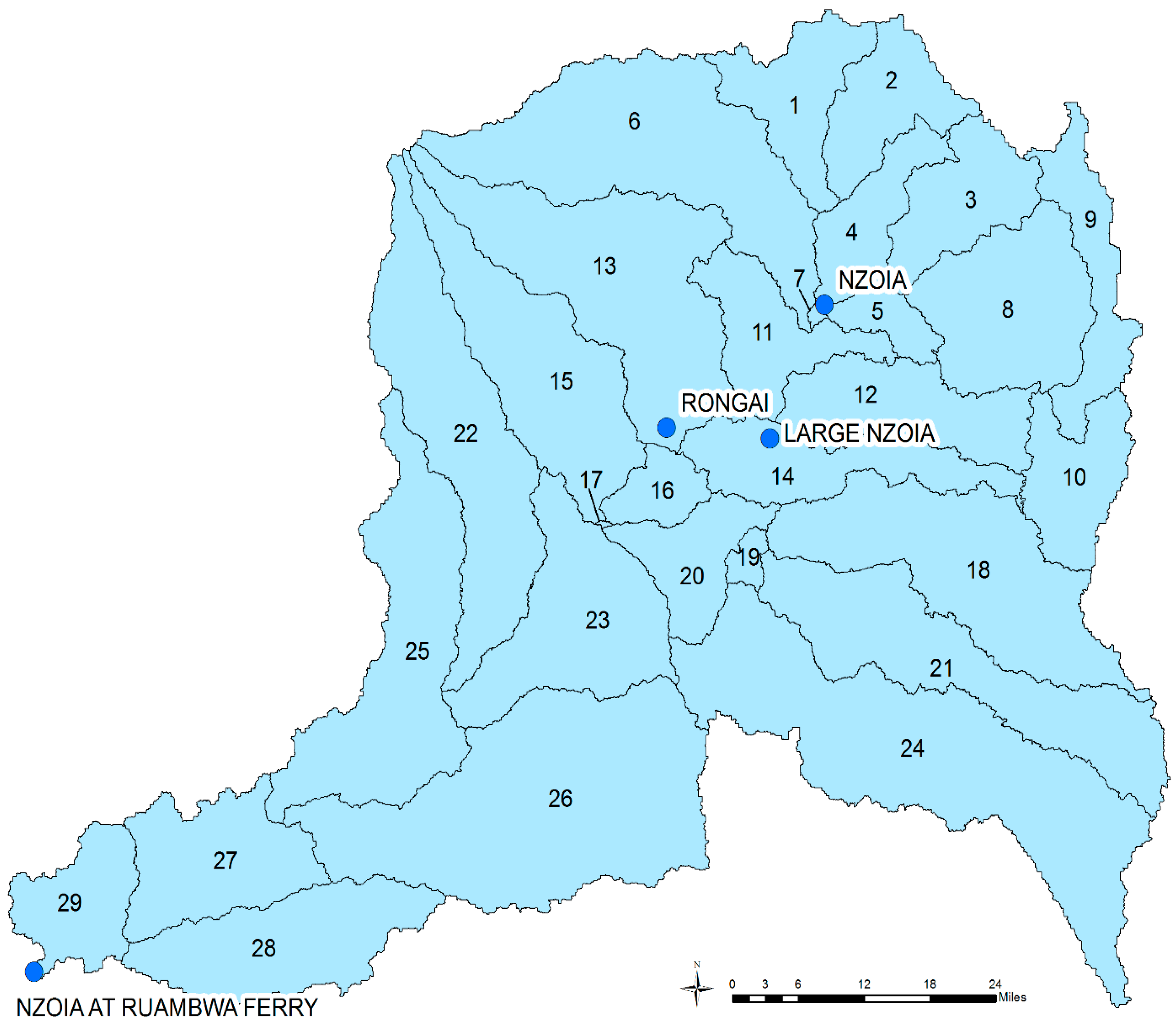
16], the Nzoia Basin (latitudes 1°30′ N and 0°05′ S and longitudes 34° and 35°45′ E), covers a catchment area of over 12,000 km
2 and originates from the eastern slopes of Mount Elgon and the western slopes of the Cherangani Hills (
Figure 1). Based on basin geomorphology and land use, it can be separated into four zones: mountain zone, plateau zone transition zone, and lowland zone [
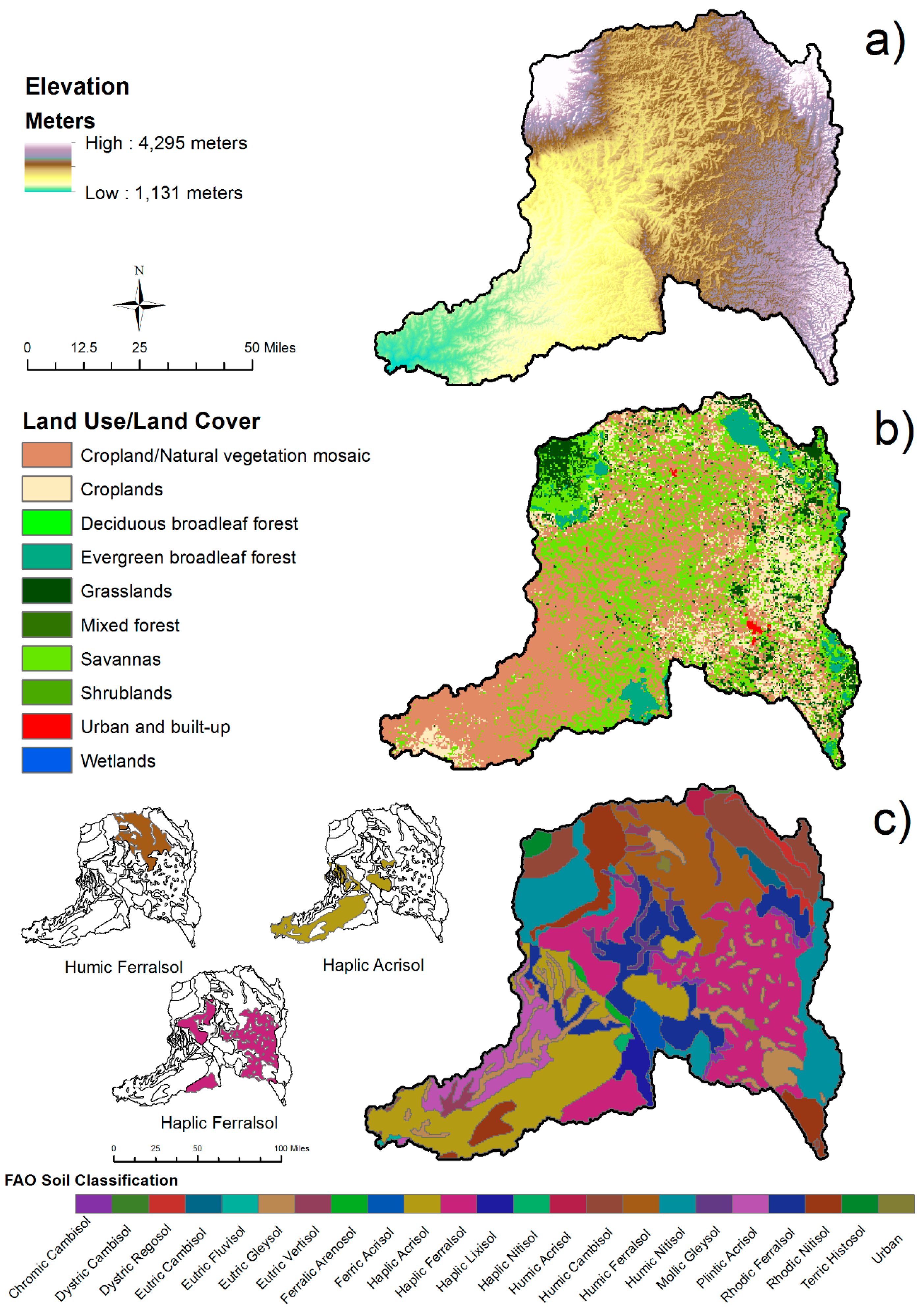
17]. The mountain zone includes the higher elevation regions of Mount Elgon and the Cherangani Hills, and the plateau zone is the major farming region within the basin with smaller-scale farming continuing into the transition and lowland zones. The lowland zone also experiences perennial flooding due to its slopes and soils. The two most dominant soil types within the basin are acrisols and ferralsols. Acrisols are found in the low-lying areas close to the outlet of the basin. They often create a hard surface crust, which causes insufficient penetration of water during precipitation events and adds significantly to the region’s flooding potential. Ferralsols are a less weathered version of acrisols and found upstream from them in the higher elevation regions of the basin. Ferralsols have a limited capacity to hold “available” water, which is harmful to crop growth and during periods of drought. The average rainfall for the basin is about 1424 mm, with high rainfall amounts between 1500 and 1750 mm occurring at higher elevations (Mount Elgon and Cherangani Hills) and lower rainfall amounts between 800 and 1100 mm in the lower reaches of the catchment [
18]. Although Lake Victoria has a unique influence on the basin’s local climate [
19], there are generally four distinct seasons (two rainy and two dry) throughout the year based on the annual shifting of the inter-tropical convergence zone (ITCZ).
Currently, ~90% of the basin’s inhabitants rely on subsistence agriculture and livestock for their livelihood [
20], resulting in over 40% of the land within the basin classified as cropland (based on the International Geosphere-Biosphere Programme classifications). The Nzoia Basin expects urban growth and has a medium to high potential for industrial agricultural schemes [
21] despite its significant population of more than 3 million inhabitants [
22]. Unfortunately, this growth is also paired with projected water scarcity. In 2007, Kenya’s fresh water per capita was 647 m
3, a value below the United Nations recommended 1000 m
3. Projections largely based on population growth indicate that fresh water per capita has the potential to decline to 235 m
3 by 2025 [
23].
3. Materials and Methods
In order to understand how to improve water resource assessment in relatively poorly gauged basins, the statistical performance of SWAT model streamflow estimation was compared when utilizing three different types of precipitation datasets as model inputs. The SWAT model has been used previously within the Nzoia Basin [
24,
25,
26] as it is open source and a powerful tool for water resource managers. As precipitation data is often considered the largest influence in hydrologic simulation models [
4,
5], it was important to understand the impact of variable precipitation inputs to the SWAT model within the Nzoia Basin.
The following datasets were used as inputs into the SWAT model to simulate streamflow (
Figure 2): 30 m Advanced Spaceborne Thermal Emission and Reflection Radiometer (ASTER) Global Digital Elevation Model Version 2 (GDEM V2 obtained from the Land Processes Distributed Active Archive Center (LP DAAC) Global Data Explorer), 1:1,000,000 Soil and Terrain Database for Kenya (KENSOTER v.2) from the International Soil Reference and Information Centre, Moderate Resolution Imaging Spectroradiometer (MODIS)’ 500 m land cover product (MCD12Q1), and various precipitation inputs that will be discussed more in depth. The World Agroforestry Centre (ICRAF) provided daily streamflow data for four river gauge stations (
Figure 3). The stations had data from 1971 to 2000, but none of the stations had complete records over the temporal range. The Lake Victoria Basin Commission (LVBC) provided monthly discharge data for the Nzoia at Ruambwa Ferry station over the temporal range 1974–2008 with no missing data.
3.1. Various Precipitation Inputs
This study analyzed the use of three different types of precipitation inputs: in situ station data, precipitation data derived from reanalysis of numerical weather predictions, and blended satellite and station data.
3.1.1. Rain Gauge Stations
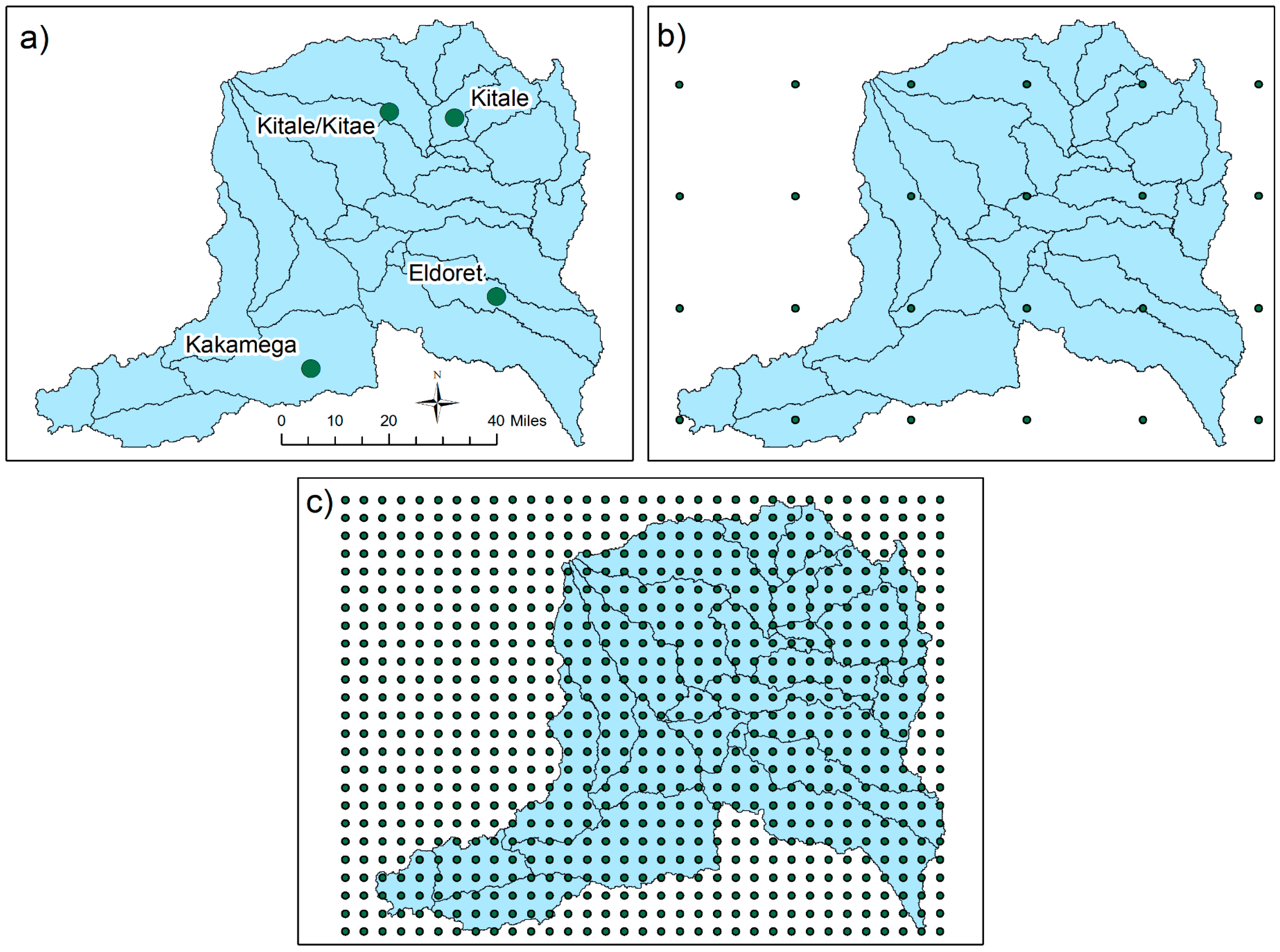
The University of California Santa Barbara’s Climate Hazards Group (CHG) provided monthly in situ rainfall data station gauge data. The spatial distribution of the four stations can be seen in
Figure 4a. Although the stations are spatially distributed adequately throughout the basin, none of the stations had complete records for the temporal range of the study. The Global Historical Climate Network (GHCN) dataset was used as the foundation for the precipitation record and any missing records were filled with Global Summary of the Day (GSOD) and World Meteorological Organization’s Global Telecommunication System (GTS) gauge data, respectively. The ranking is due to the unreliability of the GSOD and GTS datasets in comparison to the GHCN dataset [
6]. Despite the blending of station data, there were still significant gaps in the precipitation record over the temporal range. All four stations had missing data with anywhere between 30% and 65% of data missing.
3.1.2. CFSR Dataset
The National Centers for Environmental Prediction (NCEP) CFSR daily meteorological dataset was compiled with a 38 km horizontal resolution. The dataset is derived from the reanalysis of a global, high resolution, coupled atmosphere-ocean-land surface-sea ice system. The reanalysis occurs every 6 h and incorporates previously predicted forecast data and data from the analysis used to create the upcoming forecast in order to eliminate trends that never came to pass. The spatial distribution of the 30 CFSR data locations throughout the Nzoia Basin is shown in
Figure 4b. The dataset is available on the SWAT website and is recommended by the developers. However, although SWAT developers recommend the CFSR dataset, a study comparing different precipitation products in a watershed in eastern Africa found that the CFSR dataset in particular had poor spatial correlation in comparison to satellite-derived and interpolated gauge precipitation datasets. In addition, the size of the Nzoia Basin (12,000 km
2) may not be suitable for the use of reanalysis data without downscaling the data [
27].
3.1.3. CHIRPS Dataset
The CHIRPS dataset is a relatively new quasi-global, high resolution, daily, pentadal, and monthly precipitation dataset. The dataset is unique in that it provides low latency, long recorded high resolution gridded data and allows scientists to both analyze current trends and compare them to historic trends on the scale appropriate for watershed management [
6]. Essentially, CHIRPS uses a fixed Cold Cloud Duration (CCD) value threshold and regression techniques based off of Tropical Rainfall Measuring Mission (TRMM) Multi-Satellite Precipitation Analysis (TMPA) data to create rainfall estimates that are blended with in situ station data using a modified inverse distance weighted algorithm [
28]. The incorporation of station data also helps to correct for estimates that often underestimate the intensity of precipitation events. It should be noted that since the CHIRPS dataset was first published in 2015, there are very few studies that evaluate and compare the CHIRPS dataset with similar global precipitation datasets. Even a recent study in eastern Africa from 2016 [
27] comparing global precipitation datasets as an alternative to gauge data did not include the CHIRPS dataset in their analysis. Although not geographically relevant to this study, Duan et al. [
29] compared three different types of precipitation products for a small watershed in Italy: interpolated gauge station information like the Global Precipitation Climatology Centre (GPCC) data, datasets based off of numerical weather predictions and atmospheric models like the CFSR product, and datasets created from a blend of satellite-derived information and gauge station information like TRMM and CHIRPS. Overall, the study found that the CHIRPS dataset, at the 0.05° spatial resolution, showed the smallest bias and relatively better performance than all of the other precipitation products. Furthermore, the 0.05° resolution (currently the lowest spatial resolution of all of the satellite-derived global precipitation datasets) of the CHIRPS data makes it a favorable dataset for application in hydrological models at small basin scales.
CHIRPS data is available on the Climate Hazard Group’s File Transfer Protocol (FTP) site in a variety of spatial and temporal resolutions and file formats. Daily precipitation .tif files were downloaded from the FTP site at a 0.05° resolution. The SWAT model requires climate inputs as text files. As a result, the Mapping Toolbox within MATLAB was used to create a “station” at every pixel of the precipitation .tif file in order to read the precipitation information into a sequential text file. The Mapping Toolbox in conjunction with the basin’s DEM were necessary for maintaining the 3-dimensional spatial location of each “station”. After processing, there were a total of 825 stations throughout the study area (
Figure 4c).
3.1.4. Precipitation Dataset Comparison
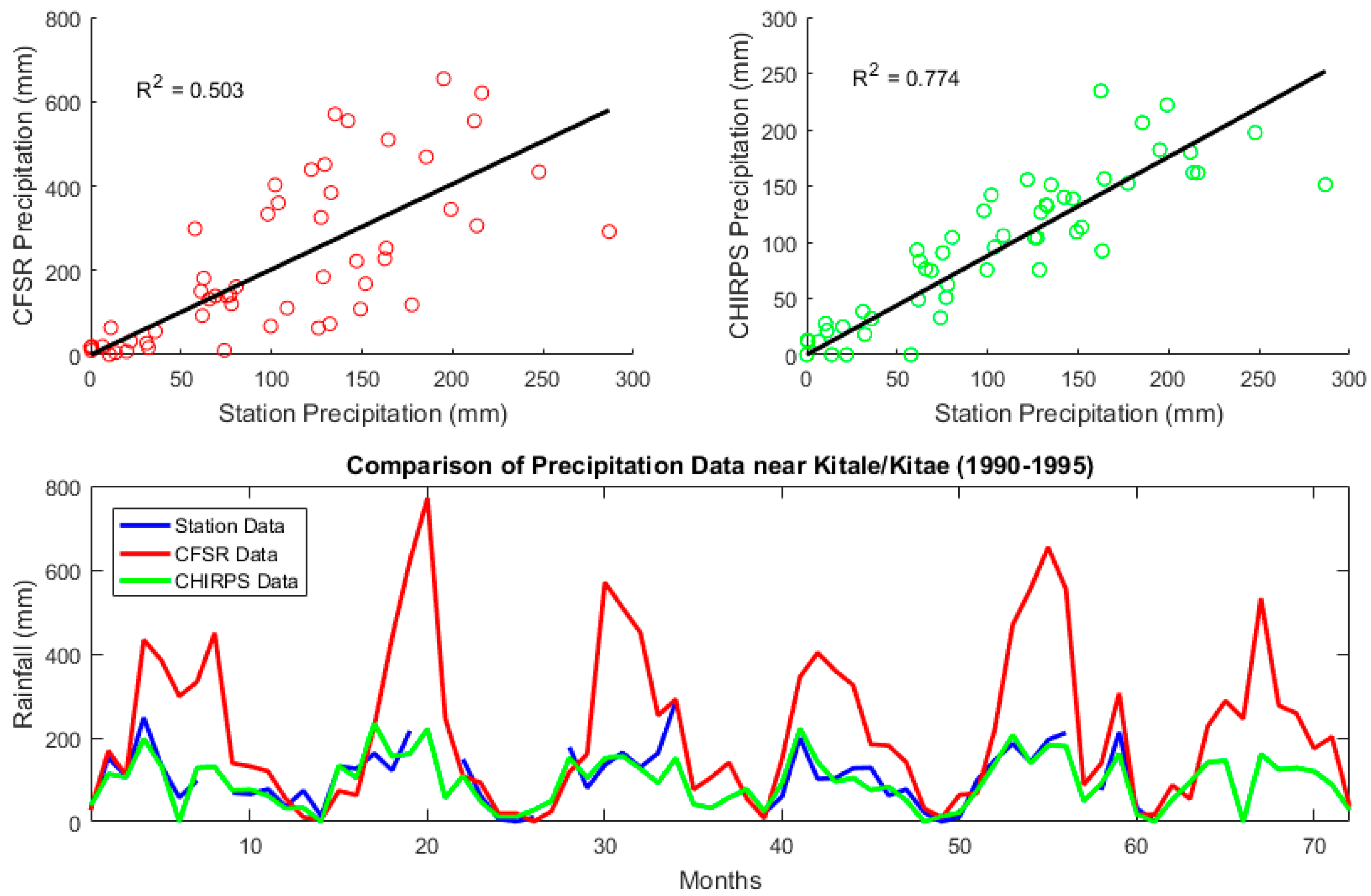
Of the four stations providing precipitation information, Kitale/Kitae had the least complete records with about 65% of the data missing. Precipitation records of in situ station data, CFSR reanalysis, and satellite-derived CHIRPS data were compared at stations with the closest proximity to the Kitale/Kitae station over the temporal range (
Figure 5). As shown, the CHIRPS dataset had a greater temporal correlation with the in situ station data than the CFSR dataset. As mentioned previously, this is likely due to the CFSR dataset’s poor spatial correlation and unsuitability for small-scale watershed studies. However, although the CHIRPS dataset does match the in situ station better than the CFSR dataset, it still consistently overpredicted rainfall during wetter periods and reported 0 mm of rainfall in months that the in situ station dataset reported anywhere between 13.7 and 57.67 mm of rainfall. Overall, since the CHIRPS dataset had the higher correlation with the gauge station data and it had the greatest spatial density (
Figure 4) and temporal consistency (
Figure 5) of all three datasets, it was hypothesized that the CHIRPS dataset would be the most complete and accurate dataset for hydrologic modeling within the Nzoia Basin.
3.2. SWAT Model
The SWAT model is a semi-distributed and time continuous watershed simulation tool that operates on a daily time step. The tool is largely based off of the concept of hydrologic response units (HRUs). The DEM is used to define the watershed boundary and drainage network. Then, the watershed in question is first discretized into subwatersheds, and further discretized into HRUs that are defined by unique land use/land cover, slope, and soil attributes [
30]. After discretization and the input of climate parameters (precipitation, air temperature, relative humidity, wind speed, and solar radiation), the following water balance equation is applied daily to each individual HRU:
where
t is time in days,
SW is soil water content, and
R,
Q,
ET,
P, and
QR are daily amounts (mm) of precipitation, runoff, evapotranspiration, percolation, and groundwater flow, respectively. It is important to note that, of the climate parameters, precipitation was the only parameter that changed between model iterations. The CFSR dataset was used for the remaining climate parameters. To maintain a continuous water balance, the model used a modified Soil Conservation Service (SCS) curve number method to simulate runoff, which is based off of curve numbers (CNs) derived from the ISRIC soil database. In addition, since the CFSR dataset provides wind speed, relative humidity, and solar radiation data, evapotranspiration could be estimated by the model using the Penman–Monteith method [
31].
The sequential uncertainty domain parameter fitting (SUFI-2) algorithm is an auto-calibration technique included within the SWAT Calibration and Uncertainty Program (SWAT-CUP) [
32].
4. Results
The accuracy of SWAT model iterations in representing streamflow was determined by comparing simulated streamflow values to measured values from discharge stations provided by ICRAF and the LVBC.
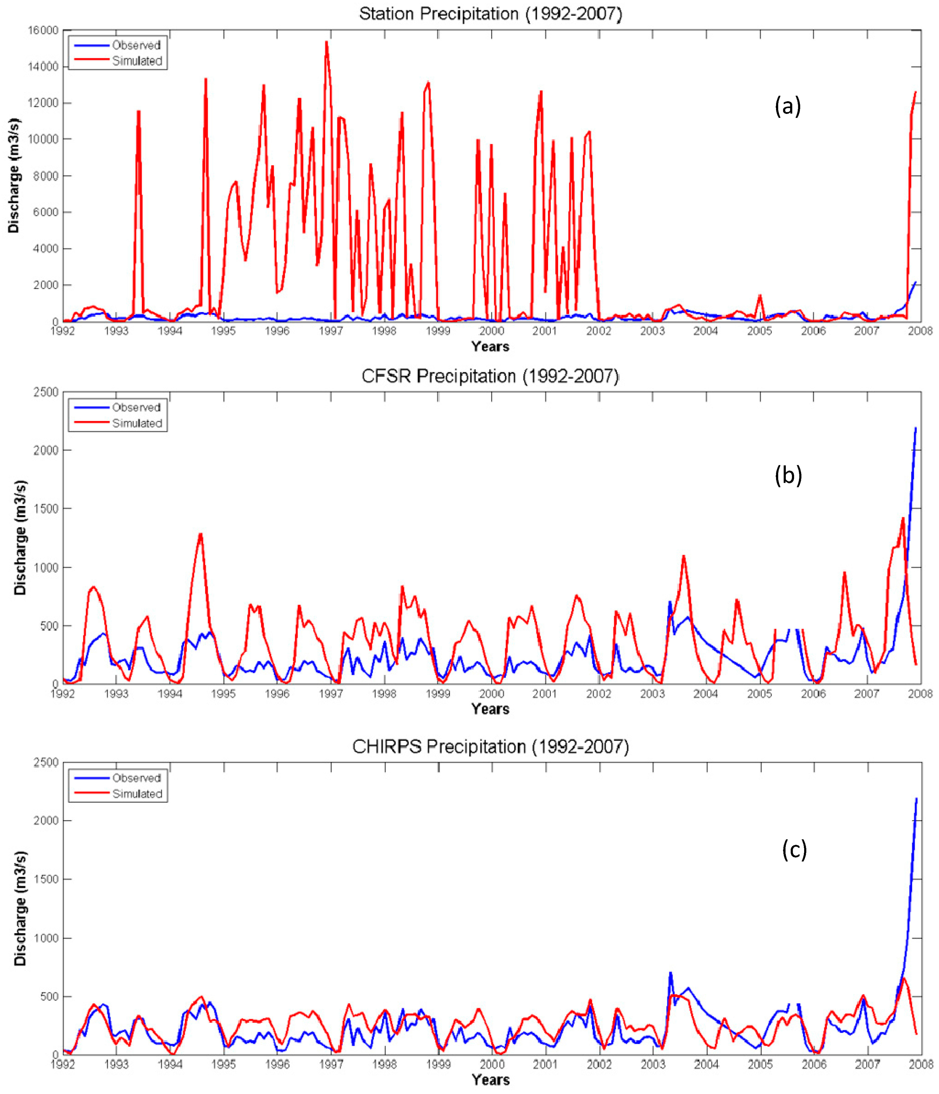
Figure 6 is a comparison of the observed monthly streamflows from the Nzoia at Ruambwa Ferry discharge station and uncalibrated simulated monthly streamflows for each of the various precipitation inputs from subbasin 29. As shown, streamflow estimation using the in situ station precipitation ranges up to 16,000 m
3/s, with the model simulation greatly overestimating streamflow. By comparison, using the CFSR and CHIRPS precipitation datasets allowed for a greater correlation of streamflow peaks. The extremely poor performance of streamflow estimation using gauge station data can be attributed to the low temporal consistency and spatial density of the data. Based on the initial comparison of SWAT model streamflow estimation, only the CFSR and CHIRPS models were calibrated over a smaller subset of the temporal range of the study.
Since the CFSR and CHIRPS datasets were available at a daily time step, model calibration (1990–1995) and validation (1996–2000) were done using daily discharge data provided by ICRAF at four different stations. After determining the sensitive hydrologic parameters to streamflow estimation, the SWAT-CUP algorithm allows the user to optimize for various statistical tests.
Table 1 indicates the sensitive parameters for each of the model runs.
Both model runs showed significant sensitivity to the SCS curve number (essentially runoff estimation), which is a common source of uncertainty for the SWAT model [
33,
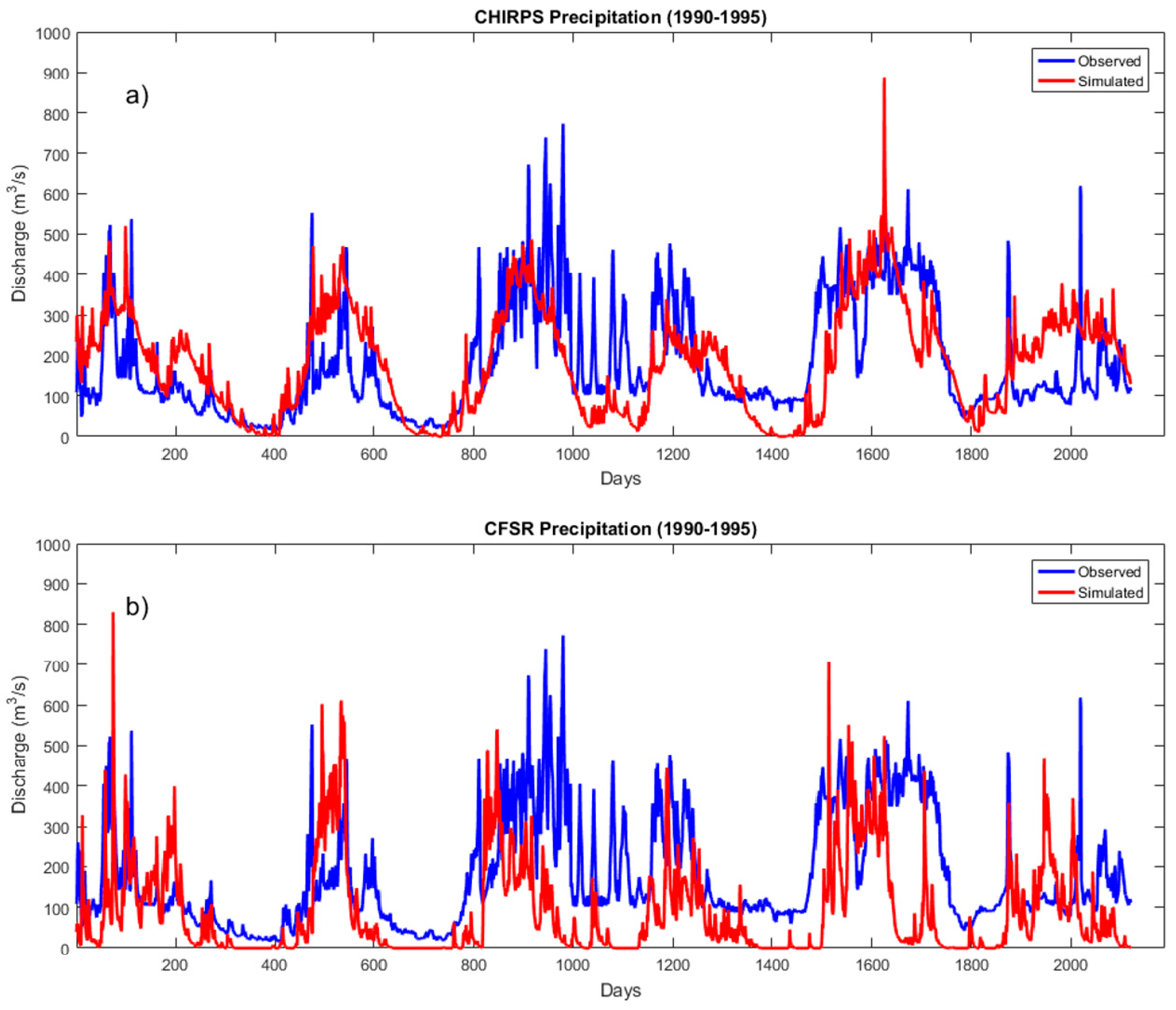
34]. The model runs using the CFSR dataset, however, showed greater sensitivity to hydrologic parameters that influence the magnitude and timing of water recharging into the groundwater system than the model runs using the CHIRPS dataset (GW_DELAY, ALPHA_BF, and RCHRG_DP). The precipitation analysis at the Kitale/Kitae station showed that the CFSR dataset was overpredicting rainfall estimates more during wetter months than the CHIRPS dataset. When the CFSR dataset was used as an input to the SWAT model, however, streamflow was more frequently underestimated during dry periods in comparison to SWAT model runs using the CHIRPS dataset (
Figure 7). Therefore, it is likely that, in order to compensate for the greater amount of rainfall during the wetter months, the CFSR model runs were depending heavily on changing parameter values for hydrologic processes related to groundwater processes.
The two statistical criteria that were used for evaluating model estimation of streamflow were the Nash–Sutcliffe Efficiency (NSE) and the coefficient of determination (R
2). The NSE is one of the most highly used criteria for comparing hydrologic model performance with observed values and can be deconstructed into three different components: linear correlation (r, ideal value = 1), normalized bias (β, ideal value = 0), and relative variability (α, ideal value = 1) [
35]. As shown in
Table 2, although streamflow estimation using the CFSR dataset resulted in reasonable R
2 values, streamflow estimation using the CHIRPS dataset resulted in equally reasonable R
2 values but improved NSE values by comparison. Parameter ranges that were used to achieve the calibrated streamflow estimates with CHIRPS data were then used for the validation period (1996–2000) and the statistical performance can also be found in
Table 2.
5. Discussion
Although the results show that the incorporation of remote sensing-based precipitation data resulted in improvements compared to the station precipitation model run, the CHIRPS model run did not consistently outperform the CFSR model run. The CFSR model run resulted in improved R
2 values at the Nzoia location, a discharge station located in the higher slope regions of the basin (
Figure 3). The CSFR model run was likely better at depicting precipitation in this region because satellite-derived precipitation estimates have been found to have limitations in mountainous regions of East Africa [
36]. Typically, rainfall estimates derived from thermal infrared (TIR) have difficulty discriminating between raining and non-raining clouds as orographic clouds that produce precipitation are often warm. Algorithms that rely on data from passive microwave sensors are also subject to misidentification based on the appearance of ice within clouds [
37]. The CHIRPS dataset references five satellite products that include information from microwave and infrared wavelengths [
6]. As a result, the CHIRPS dataset could be providing less accurate estimates of precipitation in the higher slope regions of the Nzoia Basin and impacting streamflow estimation, which could explain the difference in estimation efficiency shown in
Figure 8.
It is important to note, however, that the literature for the CHIRPS dataset does not suggest that its performance in complex topography is poor [
6,
38]. When comparing the performance of the various statistical tests for the CFSR and CHIRPS model runs, the mathematical measure of the efficiency criteria is important. The coefficient of determination (R
2) is used to understand how much of the observed variance is expressed in the simulated data. Therefore, high R
2 values can be obtained even when there is a relatively significant difference between simulated and observed magnitudes as long as the timing and shape of the magnitudes are present. The efficiency E from the NSE statistical test is a sum of the absolute squared differences between predicted and observed data normalized by the variance in the observed dataset [
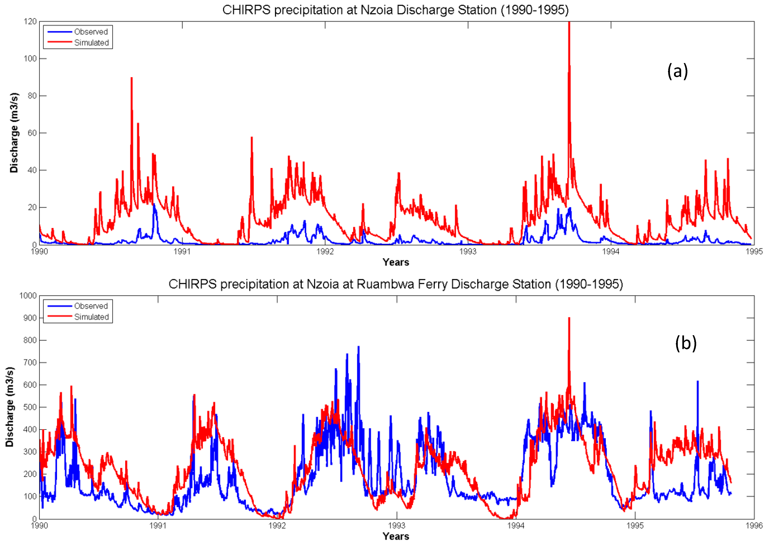
39]. Since the differences between predicted and observed data are squared, the statistical test weights larger differences more than smaller ones. For example, the R
2 values at the Nzoia discharge station and the Nzoia at Ruambwa Ferry discharge station were 0.49 and 0.38, respectively. However, it is clear that the simulated streamflow at the Nzoia discharge station (
Figure 8a) overestimated flows to a greater magnitude during wetter periods. In contrast, the magnitude of flows was matched more accurately at the Nzoia at Ruambwa Ferry discharge station (
Figure 8b).
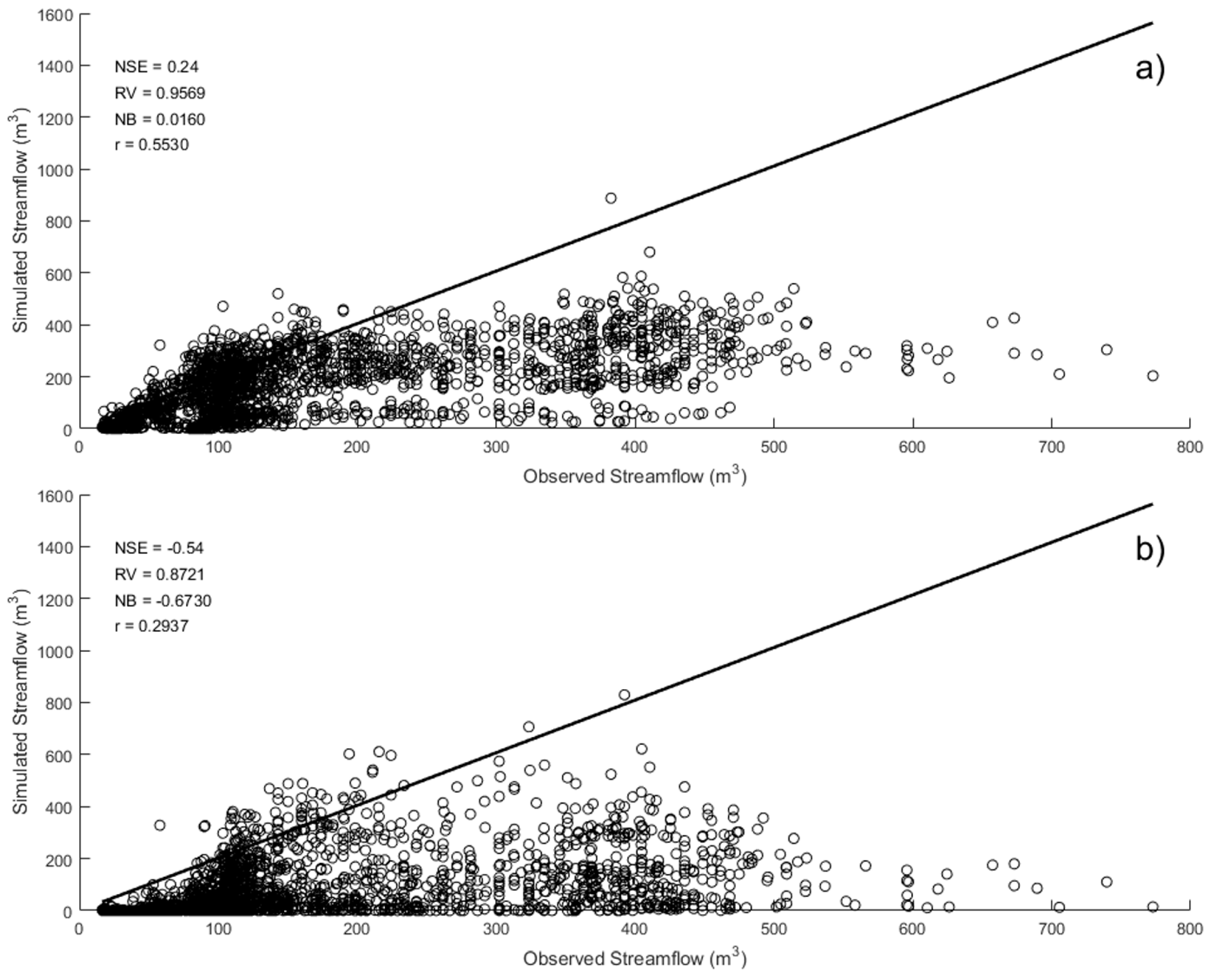
Lastly, especially with low and negative NSE values, decomposition of the NSE can provide important statistical insight as to why model simulation of streamflow is or is not matching observed values.
Figure 9 shows the temporal correlation between observed streamflow and simulated streamflows using the CHIRPS and CFSR datasets. The streamflow estimation using the CFSR dataset had more data points falling along the area near the regression line as streamflow increased, but streamflow estimation using the CHIRPS dataset had a better correlation with observed streamflow when flows were less than 200 m
3, a pattern observed in
Figure 7 as well. The values for relative variability can be considered “good” for both streamflow estimations, indicating that neither precipitation datasets resulted in anomalously high streamflow values. The values for normalized bias, however, were much better for streamflow estimates using the CHIRPS dataset than for streamflow estimates using the CSFR dataset. The bias within the streamflow estimates using the CFSR dataset could be linked back to the dataset’s overestimation of precipitation in the wetter months. Finally, although the linear correlation value that indicates the simulation data’s ability to reproduce the timing and shape of discharge is greater for streamflow estimates using the CHIRPS dataset, it is still not ideal and explains why the overall NSE value is so low. The inability to reproduce timing and shape of discharge can be linked to the CHIRPS dataset’s tendency to consistently overpredict rainfall during wetter months and anomalously report 0 mm of rainfall during some dry periods.


