Article

Automated Extraction of Urban Water Bodies from ZY‐3 Multi‐Spectral Imagery

1
School of Geomatics, Liaoning Technical University, Fuxin 123000, China
2
Satellite Surveying and Mapping Application Center, National Administration of Surveying, Mapping and Geoinformation, Beijing 100048, China
*
Author to whom correspondence should be addressed.
Water 2017, 9(2), 144; https://doi.org/10.3390/w9020144
Submission received: 31 October 2016 / Accepted: 14 February 2017 / Published: 21 February 2017

Abstract

:
The extraction of urban water bodies from high-resolution remote sensing images, which has been a hotspot in researches, has drawn a lot of attention both domestic and abroad. A challenging issue is to distinguish the shadow of high-rise buildings from water bodies. To tackle this issue, we propose the automatic urban water extraction method (AUWEM) to extract urban water bodies from high-resolution remote sensing images. First, in order to improve the extraction accuracy, we refine the NDWI algorithm. Instead of Band2 in NDWI, we select the first principal component after PCA transformation as well as Band1 for ZY-3 multi-spectral image data to construct two new indices, namely NNDWI1, which is sensitive to turbid water, and NNDWI2, which is sensitive to the water body whose spectral information is interfered by vegetation. We superimpose the image threshold segmentation results generated by applying NNDWI1 and NNDWI2, then detect and remove the shadows in the small areas of the segmentation results using object-oriented shadow detection technology, and finally obtain the results of the urban water extraction. By comparing the Maximum Likelihood Method (MaxLike) and NDWI, we find that the average Kappa coefficients of AUWEM, NDWI and MaxLike in the five experimental areas are about 93%, 86.2% and 88.6%, respectively. AUWEM exhibits lower omission error rates and commission error rates compared with the NDWI and MaxLike. The average total error rates of the three methods are about 11.9%, 18.2%, and 22.1%, respectively. AUWEM not only shows higher water edge detection accuracy, but it also is relatively stable with the change of threshold. Therefore, it can satisfy demands of extracting water bodies from ZY-3 images.

1. Introduction

Cities are the crystallization of highly developed civilization. As an important factor in the urban ecosystem, water bodies play a critical role in maintaining stability of the urban ecosystem [1]. Their changes are closely related with people’s life. Negative changes may lead to disasters, pollution, water shortage, or even epidemics [2]. Therefore, understanding the distribution and changes of urban water has become the focus of people’s attention.
In recent years, with the development and application of remote sensing technology, it has played an increasingly important role in natural resource surveying [3,4], dynamic monitoring [5,6], and natural surface water planning [7,8], thus attracting researchers’ attention. Remote sensing images enable us to observe the earth from a totally different perspective and monitor its real-time changes. Water bodies are common ground object in remote sensing images, the rapid acquisition of their dynamic information is apparently valuable for water resource survey, water conservancy planning and environmental monitoring and protection [9]. Among current water extraction technologies, a mainstream method is using remote sensing data to gather urban water information in a timely and accurate way [10]. Thus far, researchers have proposed many methods to extract water using remote sensing images [10,11]. These models could be roughly divided into four categories: (a) single-band or multiple-band threshold methods [12,13]; (b) water indices [14,15,16]; (c) linear un-mixing models [17]; and (d) supervised or unsupervised classification methods [18,19]. Other methods that are not as frequent used as the above include water extraction technology based on digital elevation models [20,21], microwave remote sensing imagery [22,23,24] and object oriented technology [25,26]. In general, the water indices are most commonly used in practice because of their simple, convenient and fairly accurate algorithm models [27].
The water indices are under constant refinement. The first model, Normalized Difference Water Index (NDWI), proposed by McFeeters [16], is based on the principle of Normalized Difference Vegetation Index (NDVI). Its basic idea is to extract water bodies by enhancing water information and suppressing non-water information. Xu Hanqiu [17] found that the NDWI algorithm could not effectively inhibit the impact of buildings and proposed a refined version, in which he used the Shortwave Infrared (SWIR) instead of the NIR in the original NDWI algorithm. The new algorithm was called the Modified Normalized Difference Water Index (MNDWI). It exhibits higher accuracy, but it still could not distinguish shadows. Therefore, Feyisa G L [18] proposed a method called the automated water extraction index (AWEI) to adapt to different environments. Five bands of Landsat5 Thematic Mapper (Band1, Band2, Band4, Band5, and Band7) were used to compute the index to enhance the contrast between water and non-water information which could be used to model the water images with or without shadows.
Most of the algorithms, however, are proposed based on medium- or low-resolution remote sensing images. Because of resolution limitations, smaller water bodies cannot be extracted effectively, especially in urban areas where the size of water bodies varies and there are many small artificial lakes and rivers [28]. Therefore, we should prioritize the use of high-resolution remote sensing images in those areas. The ZY-3 satellite is China’s first civil high-resolution stereo mapping satellite launched in 9 December 2012. Equipped with four sets of optical cameras, it includes an orthographic panchromatic time delay and integration charge-coupled device (TDI CCD) camera with the ground resolution of 2.1 m, two front-view and rear-view panchromatic TDI CCD cameras with the ground resolution of 3.6 m, and an orthographic multi-spectral camera with the ground resolution of 5.8 m. The acquired data are mainly used for topographic mapping [29], digital elevation modeling [30] and resource investigation [31]. Therefore, it is an ideal multi-spectral image data source for urban water extraction [31].
Recently, with the increase of image resolution, most of the high-resolution remote sensing images (such as those from WorldView-2, IKONOS, RapidEye and ZY-3 satellites) do not have so many available bands for water extraction compared with those from LandsatTM/ETM+/OLI imagery, rendering the MNDWI and AWEI algorithms useless. After all, most high-resolution remote sensing images only have four bands (blue, green, red and near-infrared), lacking the SWIR necessary to compute the MNDWI/AWEI indices [31]. It is therefore problematic to use the NDWI to extract urban water from high-resolution images. For instance, it is difficult to remove shadows, especially those of high-rise buildings in urban areas. The problem dramatically worsens when analyzing high-resolution images [32], thus it is difficult to distinguish between water bodies and shadows [25,33].
To tackle urban water extraction issue, some scholars have pioneered on this subject and proposed some preliminary solutions such as the object oriented technology to detect shadows by computing their texture features [34]. It can achieve expected results, but is relatively complex and time-consuming in the texture description and computation [35]. Therefore, it is not an optimal model for the shadow detection. Another method based on Support Vector Machine (SVM) feature training can be used to remove the impact of shadows on urban water extraction [31]. However, the SVM training is time-consuming, especially when there are many training samples with high-dimension eigenvectors [36]. Some researchers combine the morphological shadow index (MSI) [37] and the NDWI to extract urban water bodies from WorldView-2high-resolution imagery, in order to increase the detection accuracy [38]. The principle of this method is simple, but since the urban water extraction method is based on the NDWI algorithm, the detection accuracy is not very high, especially when detecting small areas of water surrounded by lush vegetation. In those areas, the spectral features of water will be severely contaminated and extremely unstable [39]. In addition, urban water bodies are typically sediment-laden and algae polluted, and thus exhibit different optical features compared with non-contaminated natural water bodies [31].
Therefore, to remove the limitations of traditional NDWI indices in water extraction and improve the initial classification accuracy, we propose the NNDWI1, which is sensitive to turbid water bodies, and NNDWI2, which is sensitive to water bodies whose spectral information is seriously disturbed by that of vegetation, based on the analysis of water features and shadows. To remove the disturbance of shadows of high-rise buildings to the water extraction results, and to better express the features of shadows and water bodies, we use the Object-Oriented Technology to classify the water bodies and shadows. Meanwhile, if the features expressed by the operators are too complex, it will not be conducive to reduce the computational time. Thus, it is better to use operators that express the spectral rather than textural features of ground objects in the algorithm in order to improve the computational efficiency. To further improve the efficiency, we use thresholds rather than the time-consuming classification algorithm to differentiate water bodies from shadows. The experimental results show that the automatic urban water extraction method (AUWEM) algorithm can better identify shadows and water bodies, and improve the urban water detection accuracy.

2. Study Areas and Data

2.1. Study Areas

To verify the feasibility of the automatic urban water extraction method (AUWEM) algorithm, we select five images featuring different areas with different environments including lakes and rivers within territory of China for experiments. The selected areas were located in Beijing, Guangzhou, Suzhou and Wuhan. As for Wuhan, the city is an ideal place for experiment because of its large amount of rivers and lakes as well as rich diversity of water bodies, so we select two different coverage areas for experiment. Details of the experimental areas are described in the following Table 1, and the corresponding images from ZY-3 satellite are detailed in Table 2.

2.2. Experimental ZY3 Imagery and Its Corresponding Reference Imagery

ZY-3 Images used in the experiments can be queried and ordered from http://sjfw.sasmac.cn/product/order/productsearchmap.htm. We use theZY-3 multi-spectral data to extract water. All image data are Level 1A products, which have been adjusted through radiometric and geometric correction. All the images used in the experiments were cloud free.ZY-3 satellite parameters are shown in Table 2. The experimental image information is described in the following Table 3.
The reference imagery is used to evaluate the urban water classification accuracy. To acquire the corresponding reference imagery, we manually delineate the water edge in high-resolution imagery, which is obtained by fusion of ZY-3’s high-resolution Panchromatic and ZY-3’s Multispectral Images. During the experiment, we asked an experienced analyst to manually map out the water bodies. To prevent arbitrariness, all referential images corresponding to five experimental areas were drawn by a single person. It took about 10 days, including eight days of imagery creation and two days of double-checking. Before manually mapping out water bodies and non-water areas, we collected and studied a large amount of related samples so that relevant criteria can be set up to improve the accuracy of water boundary mapping. Figure 1 shows the five referential images that are manually drawn. Here, the water bodies are in blue, and non-water area areas are in black. The relevant criteria for water body delineate are as follows:
  • Delineate precision of the fuzzy boundary of water body is within three pixels while the clear boundary of water body is within one pixels.
  • Less than or equal to one pixels of water body information is not given to delineate.
  • We choose reference of higher resolution Google map image in order to distinguish between water body and building shadow as well as the seemingly water body and non-water body.
  • Urban water system is basically interconnected with each, other except for the river intercepted by bridge.
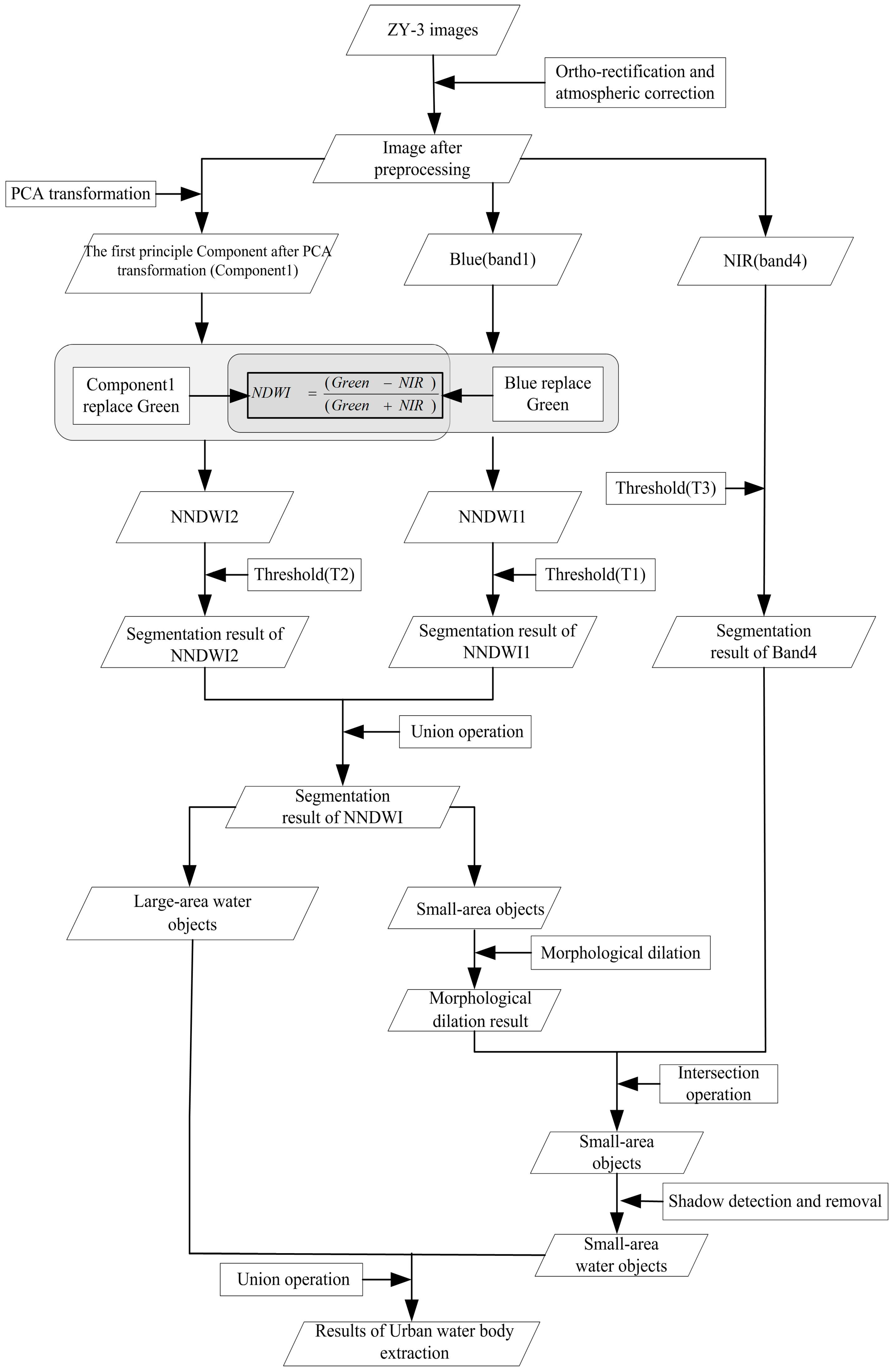
3. Method

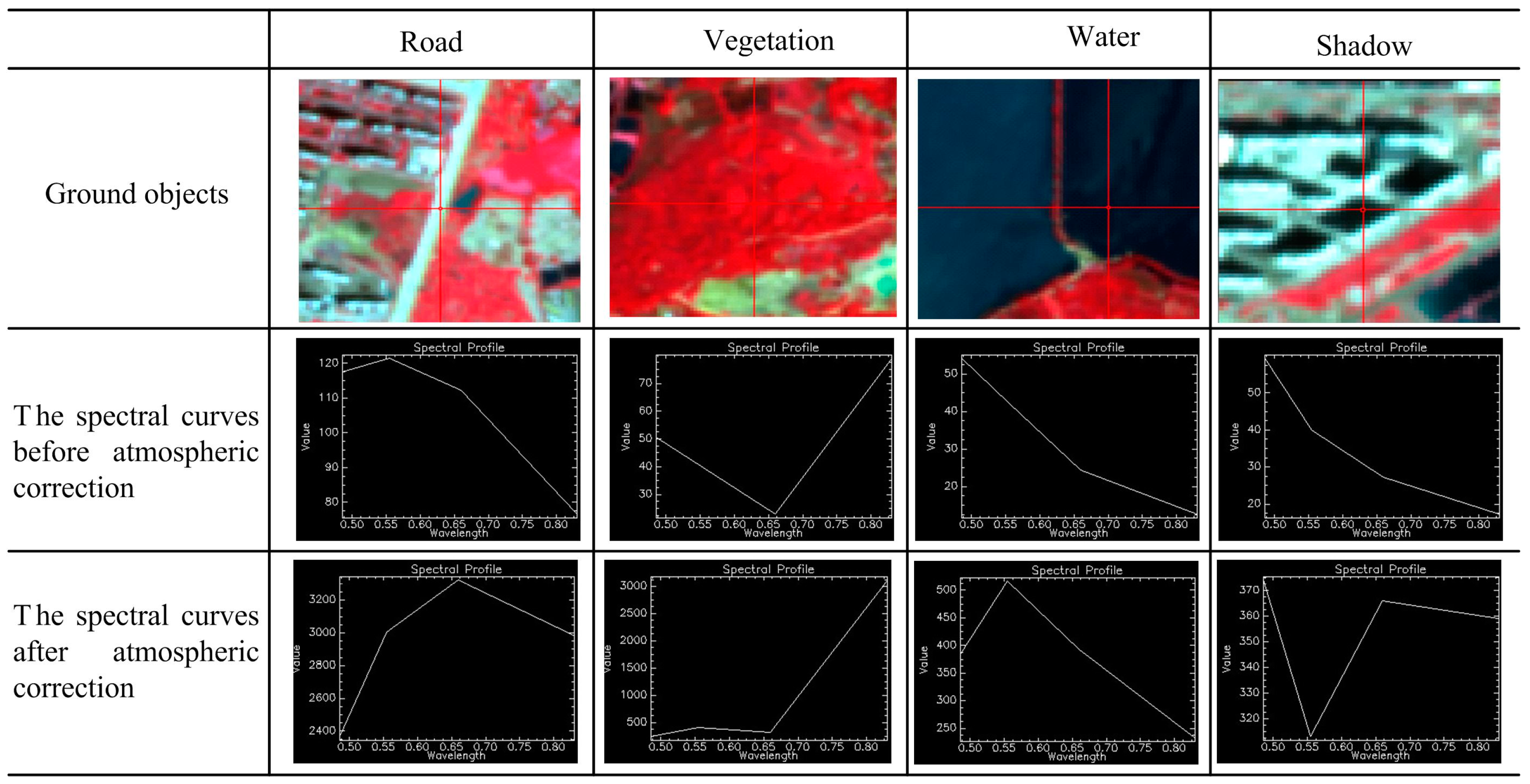
3.1. Satellite Image Preprocessing

We used in the study the level-1 imagery taken from ZY-3 satellite without Ortho-rectification, therefore we used RPC+30m DEM to process the experimental images and applied Ortho-rectification without control points. We used FLAASH (Fast Line-of-Sight Atmospheric correction model Analysis of Spectral Hypercubus) for atmospheric correction [40]. All of the above steps were completed in ENVI5.2 software.
The radiometric calibration coefficient of ZY-3 FLAASH atmospheric correction can be downloaded from http://www.cresda.com/CN/Downloads/dbcs/index.shtml. The spectral response function could be downloaded from http://www.cresda.com/CN/Downloads/gpxyhs/index.shtml.
Figure 2 depicts the spectral curves of ground objects before and after atmospheric correction. We can see from this figure that there is huge difference between the two spectral curves of pixels. The one after the atmospheric correction is more consistent with the actual features of ground objects.

3.2. Normalized Difference Water Index (NDWI)

The NDWI was first proposed by McFeeters in 1996 and successfully applied to detect the surface water in multi-spectral imagery from Landsat Multi-spectral Scanner (MSS) [14]. The definition is as follows:
N D W I = ( G r e e n N I R ) ( G r e e n + N I R )
According to this equation and the spectral feature curves of ground objects, the NDWI index value of water surface is greater than 0, the NDWI value of soil and other ground objects with high reflectivity approximately equals 0, while the NDWI value of vegetation is below 0 because the reflectivity of the vegetation on the infrared band is higher than on the green band. As a result, the water can be easily extracted from multi-spectral images.

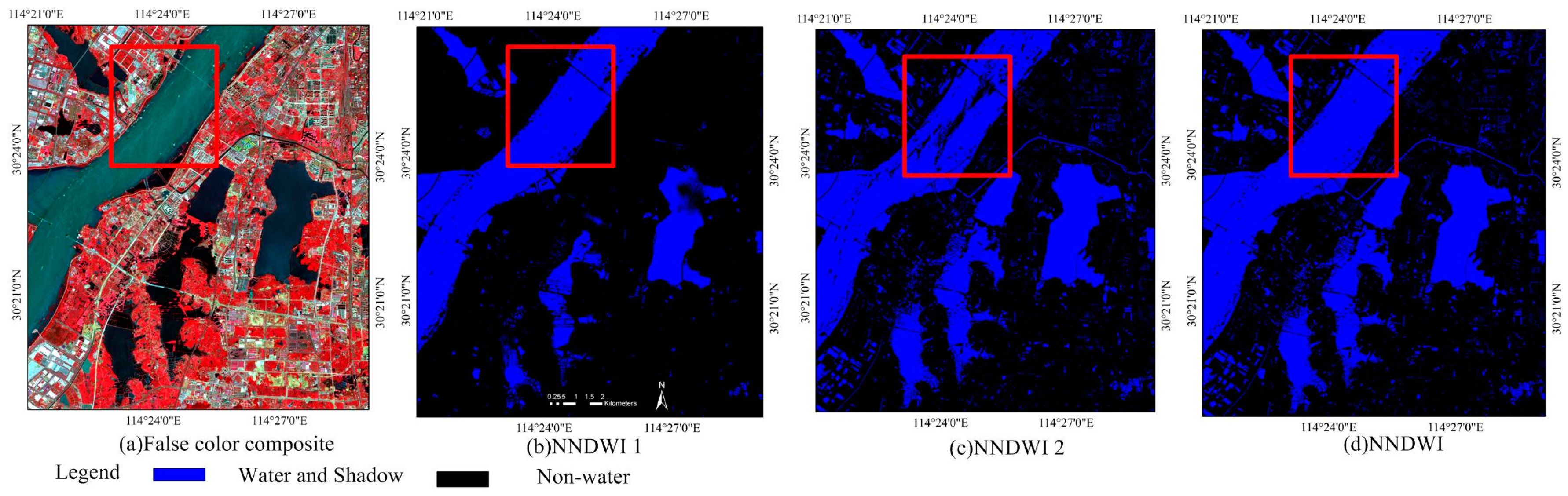
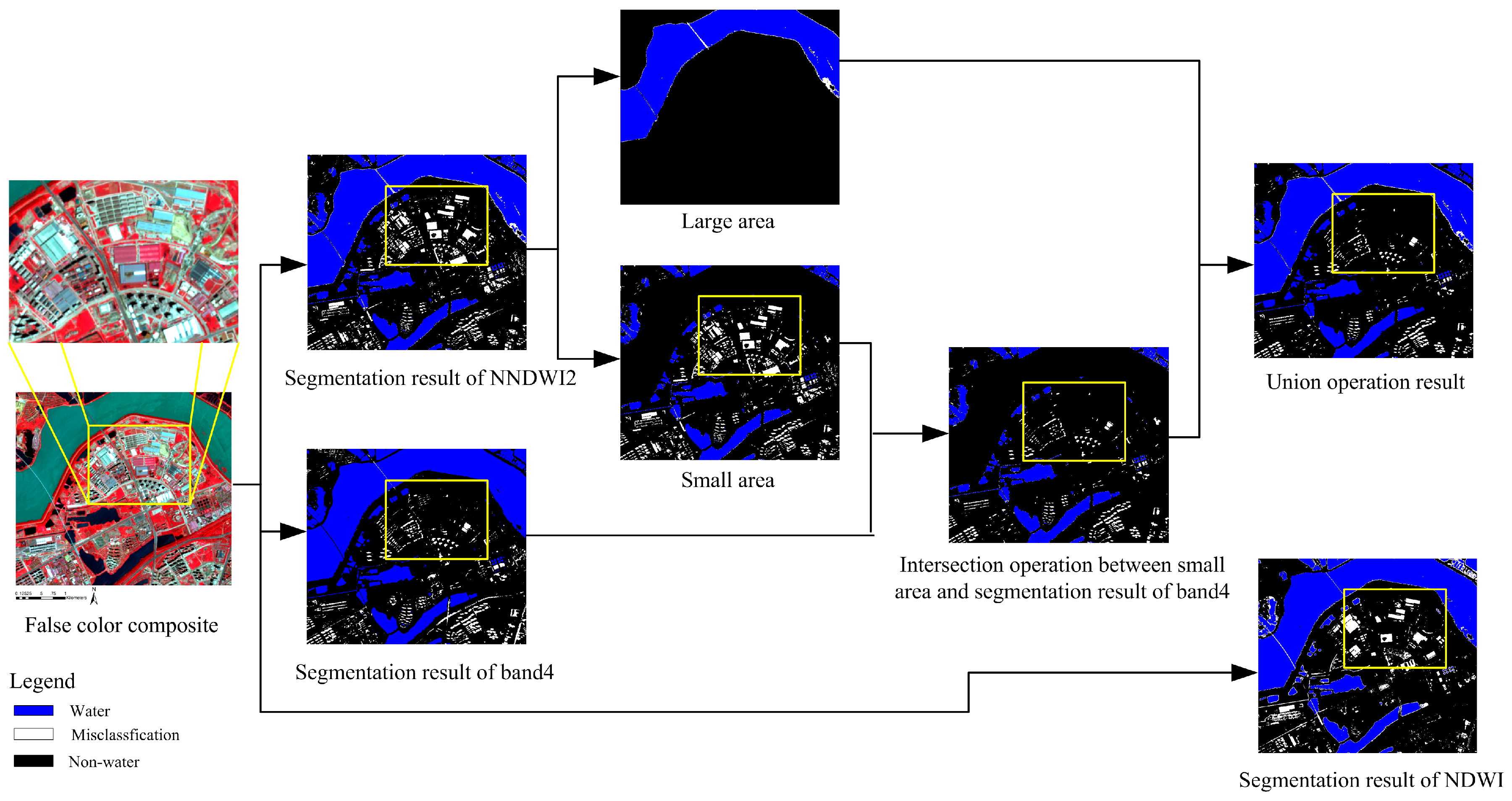
3.3. New Normalized Difference Water Indexes (NNDWI)

In our study, the computation of NNDWI comprises of two steps:
  • Use the ZY-3 Blue band (Band1) to replace the green band in Equation (1) to obtain NNDWI1, i.e.,
    N N D W I 1 = ( B l u e N I R ) ( B l u e + N I R )
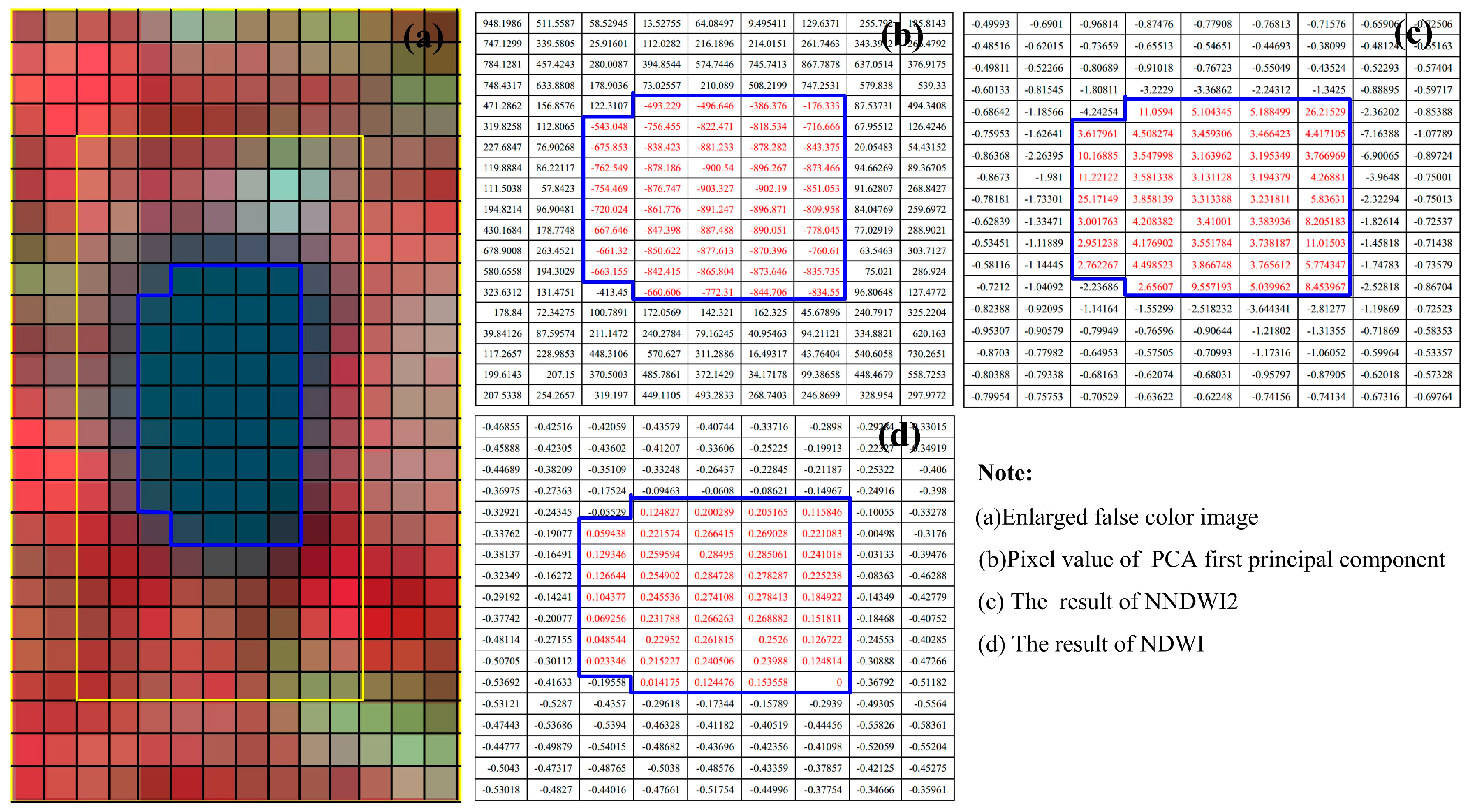
  • Four bands of ZY-3 imagery were processed by the Principal Component Analysis (PCA) transformation [41], use the first principle component after PCA transformation to replace the Green band in Equation (1) to obtain NNDWI2, i.e.,
    N N D W I 2 = ( C o m p o n e n t 1 N I R ) ( C o m p o n e n t 1 + N I R )
    where Component1 is the first principal component after PCA transformation. The PCA transformation reflects the methodology of dimension reduction [41]. From the mathematic perspective, it is to find a set of basis vectors which can most efficiently express the relations among various data. From the geometrical perspective, it is to rotate the original coordinate axis and get an orthogonal one, so that all data points reach the maximum dispersion along the new axis direction. When applied to the image analysis, it is to find as few basis images as possible to preserve the maximum information of the original images, thus achieving the purpose of feature extraction.
In our study, the initial water extraction results are generated by the superimposition of the threshold segmentation results from two water indexes, namely NNDWI1 and NNDW2. Therefore, NNDWI is expressed as follows:
N N D W I = ( s e g m e n t a t i o n _ N N D W I 1 ) ( s e g m e n t a t i o n _ N N D W I 2 )
In Equation (4), segmentation_NNDWI1 and segmentation_NNDWI2 represent the threshold segmentation results generated by NNDWI1 and NNDWI2 index image, respectively.
The result generated by NNDWI integrates the water extraction results from both algorithms, thus the omission caused by a singular index is avoided. As shown below in Figure 3, NNDWI2 algorithm is not sensitive to turbid water, whereas NNDWI1 is a complement because of its sensitivity to turbid water. Therefore, in practice, these two algorithms can be combined to generate a composite water extraction result instead of two separate ones, thus the subsequent water extraction accuracy can be enhanced.

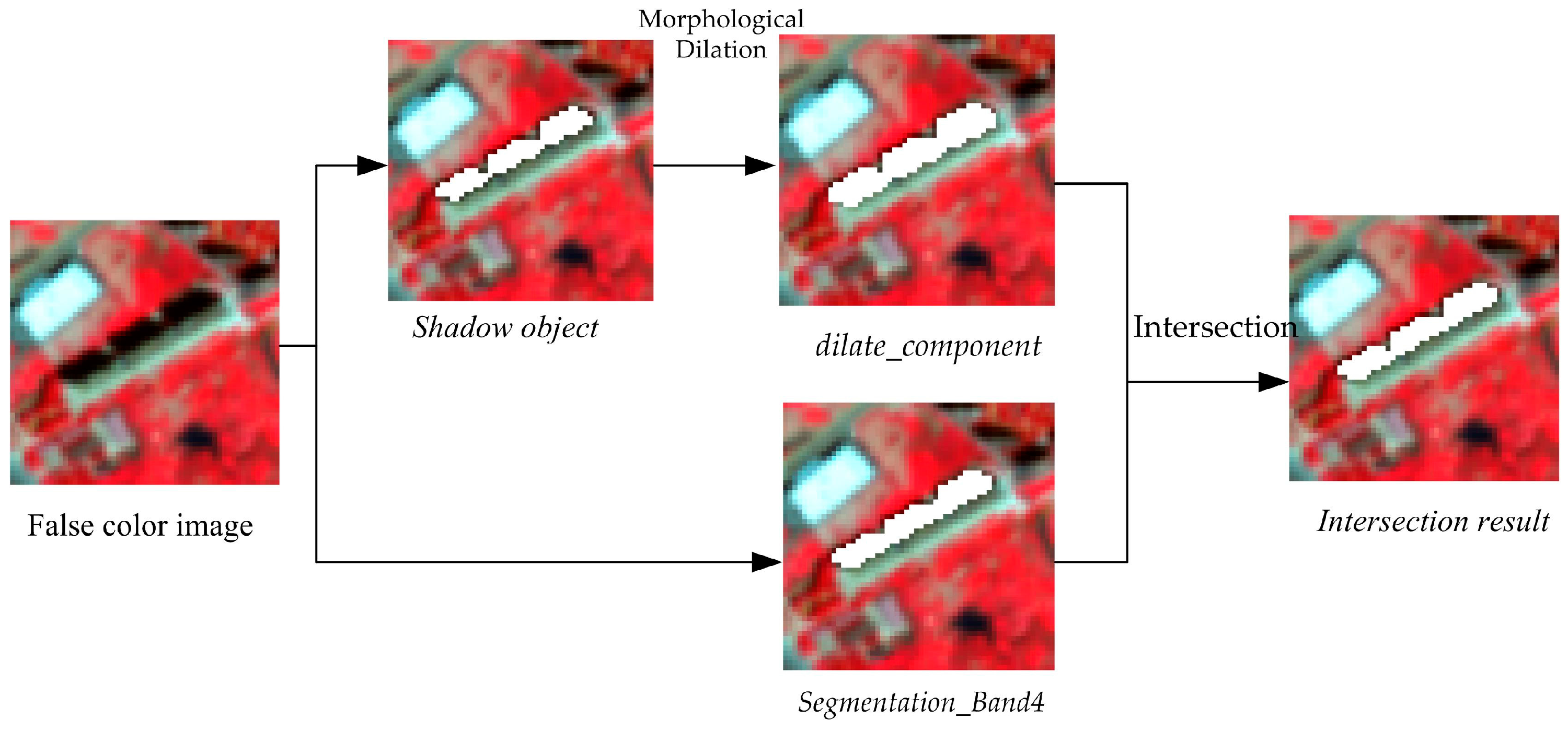
3.4. Shadow Detection Based on Object Oriented Technology

3.4.1. Shadow Objects

In the initial water extraction results generated by NNDWI, shadows are extracted along with the water bodies. While analyzing the image data extracted using NNDWI, we find that the areas of shadows are generally smaller than those of water bodies, except for some small artificial ponds and lakes in the city. Therefore, in practice, we only need to detect objects that cover small areas. These objects will encompass almost all possible shadows and small area water bodies. The model for acquiring small-area objects can be described as follows:
{ c o m p o n e n t = w a t e r i f a r e a ( c o m p o n e n t ) > t , c o m p o n e n t N N D W I c o m p o n e n t = s h a d o w o r w a t e r i f a r e a ( c o m p o n e n t ) t , c o m p o n e n t N N D W I
where t indicates the set segmentation threshold, whose value is the number of pixels that enables the maximum shadow objects; it is a minimum detectable size of water bodies that equals exclusion. The number of pixels of the largest shadow area varies in different images, resulting in different values of t, which should be set accordingly. The experimental statistics show that if we set 2000 < t < 5000, the results will be satisfactory. component indicates the discrete objects in the water extraction results generated using NNDWI, including water and shadow areas. area(component) indicates the object areas: if area(component) > t, then it indicates the water objects, while, if area(component) ≤ t, then it indicates either small area water or shadow objects.
It is impossible to extract all the shadow pixels from the water extraction results generated by using NNDWI. For better application of the Object Oriented Technology, the acquired shadow objects are under morphological dilation [42], so that the dilated objects can better include shadow pixels in the area. Meanwhile, to limit the dilation results in the actual shadow areas, we use the threshold segmentation results on the near infrared band (Band4) of ZY-3 images as the constraint. (Due to relatively low reflectivity of water and shadows on the near infrared band (Band4), the values of water and shadow pixels are relatively small. The water and shadow areas are in dark black on this band. The threshold segmentation can effectively enable the extraction of water and shadow objects. Therefore, the threshold segmentation results of Band4 serve as a constraint.) Specifically, the constraint on the dilation results is set by intersecting the dilated images and those under threshold segmentation on Band4, expressed as below:
c o m p o n e n t 2 = ( d i l a t e _ c o m p o n e n t ) ( s e g m e n t a t i o n _ B a n d 4 )
In Equation (6), the dilate_component indicates dilation results of component (i.e., the objects of water/shadow whose areas are below the threshold); and the segmentation_Band4 indicates threshold segmentation results on the near-infrared band (Band4). How the dilation results are constrained by way of intersection is shown in Figure 4.

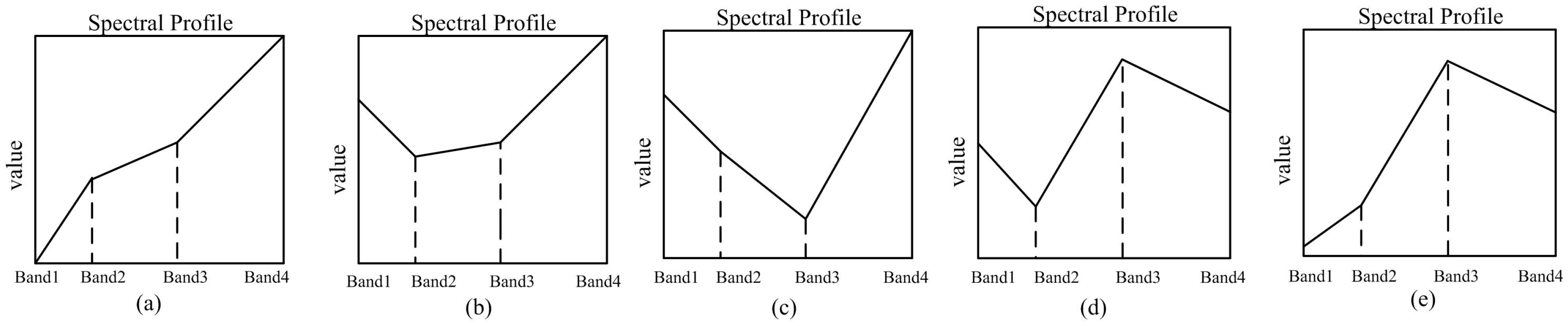
3.4.2. The Shadow Objects Description (The Description of Spectral Feature Relations between Water-Body Pixels and Shadow-Area Pixels)

Generally, the water extraction results generated by the NNDWI only cover water and shadow areas. Thus, we only need to analyze their features and find the proper ones. In the study, we find that textural features can be used to effectively describe shadows and water bodies, but those of ground objects (such as Gray Level Co-occurrence Matrix, GLCM) are complex and time-consuming to compute and thus unfit for the classification of water bodies and shadows. As a result, we use the spectral features of ground objects to describe the pixels of water and shadow areas and distinguish between them.
Through an extensive analysis of the spectral feature curves of water bodies and shadows, we find that, in general, the spectral relation of water pixels satisfies the following inequality:
Band2 > Band4
The spectral curves of shadow-area pixels are more complicated. When the sunshine is blocked by buildings, there will be shadows. The spectral features of the pixels in the shaded areas typically resemble those of other ground objects, such as vegetation, cement and soil. After analyzing the spectral features of those areas, we summarized five different spectral curve models, as shown in Figure 5.
Accordingly, we can set up the following model that shows the spectral relations of shadow pixels:
{ B a n d 2 > B a n d 1 B a n d 3 > B a n d 2 B a n d 4 > B a n d 3
{ B a n d 1 > B a n d 2 B a n d 4 > B a n d 2 B a n d 4 > B a n d 3
{ B a n d 3 > B a n d 2 B a n d 3 > B a n d 4 B a n d 4 > B a n d 2
If the spectral curves in the experimental results generated by the NNDWI index correspond with the pixels shown in the above three models, they will be classified as shadow pixels, and vice versa.

3.4.3. The Shadow Objects Detection Method

In the experiments, the classification of each small-area discrete object is determined. First, the spectral relation of each pixel of discrete objects is described to judge whether it satisfies the constraint of a shadow pixel. The number of shadow pixels in each object is recorded. According to extensive statistical experiments, we find that if the proportion of shadow pixels exceeds the threshold T, then the object can be classified as a shadow area. Otherwise, the object is classified as a water body. The judgment function can be expressed as:
{ c o m p o n e n t 2 = w a t e r i f m n T c o m p o n e n t 2 = s h a d o w i f m n > T
where n indicates the total number of pixels of an object, and m indicates the number of its shadow pixels. The threshold T is an empirical number optimized through experiments. In a statistical analysis of the shadow pixels of the ZY-3 images, we find that when T equals 0.5, water and shadow objects can be effectively differentiated.

3.5. Urban Water Extraction and Its Accuracy Evaluation

Figure 6 depicts the steps of the AUWEM algorithm. First, preprocess the imagery (by using Ortho rectification and atmospheric correction). Second, use the NNDWI described in Section 3.3 to obtain the initial water extraction results. Third, use the shadow detection method of the Object Oriented Technology detailed in Section 3.4 to detect shadow objects. Finally, remove detected shadow objects to obtain the final results of urban water extraction. The overall flow chart of AUWEM is shown in Figure 6. In order to compare image classification accuracy, we use six indicators to describe the extraction accuracy of different algorithms, including producer accuracy, user accuracy, Kappa coefficient, omission error, commission error and total error.

4. Experimental Results and Analysis

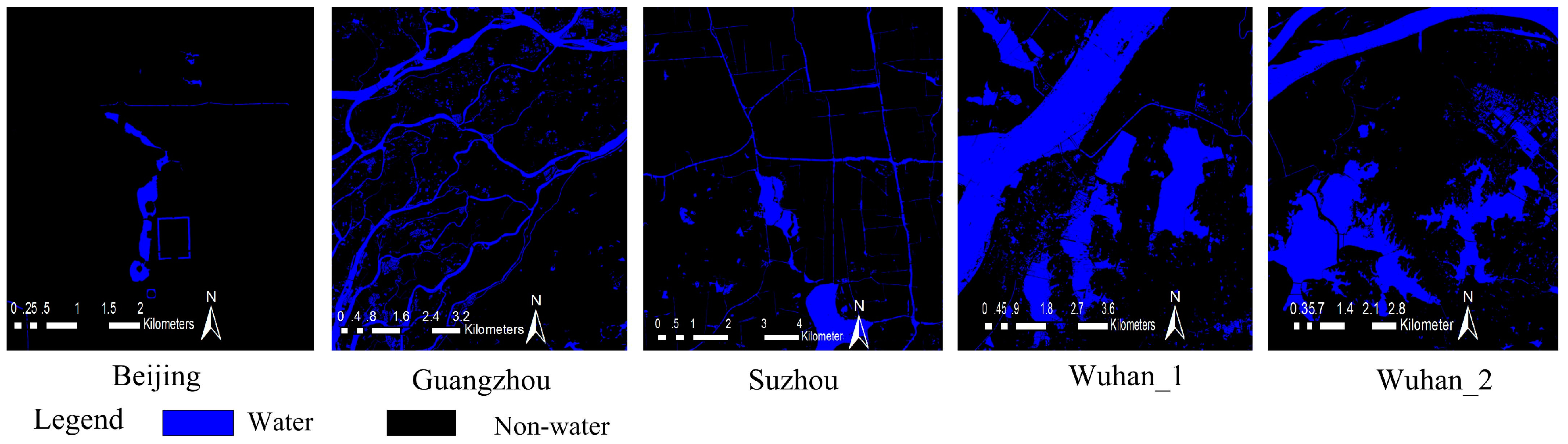
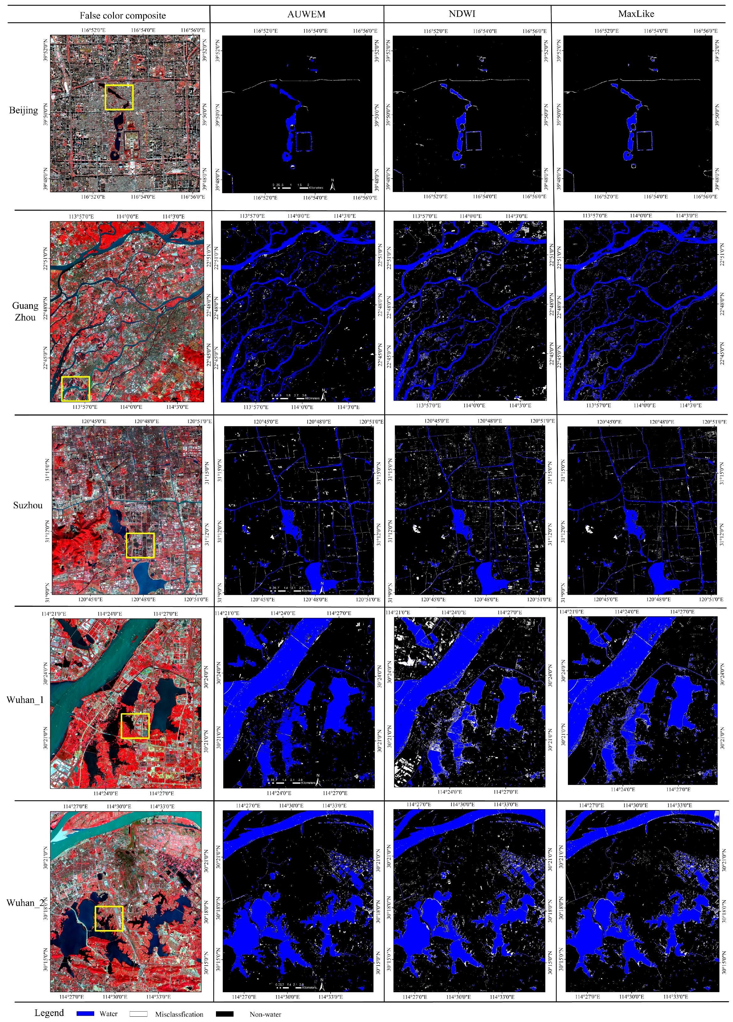
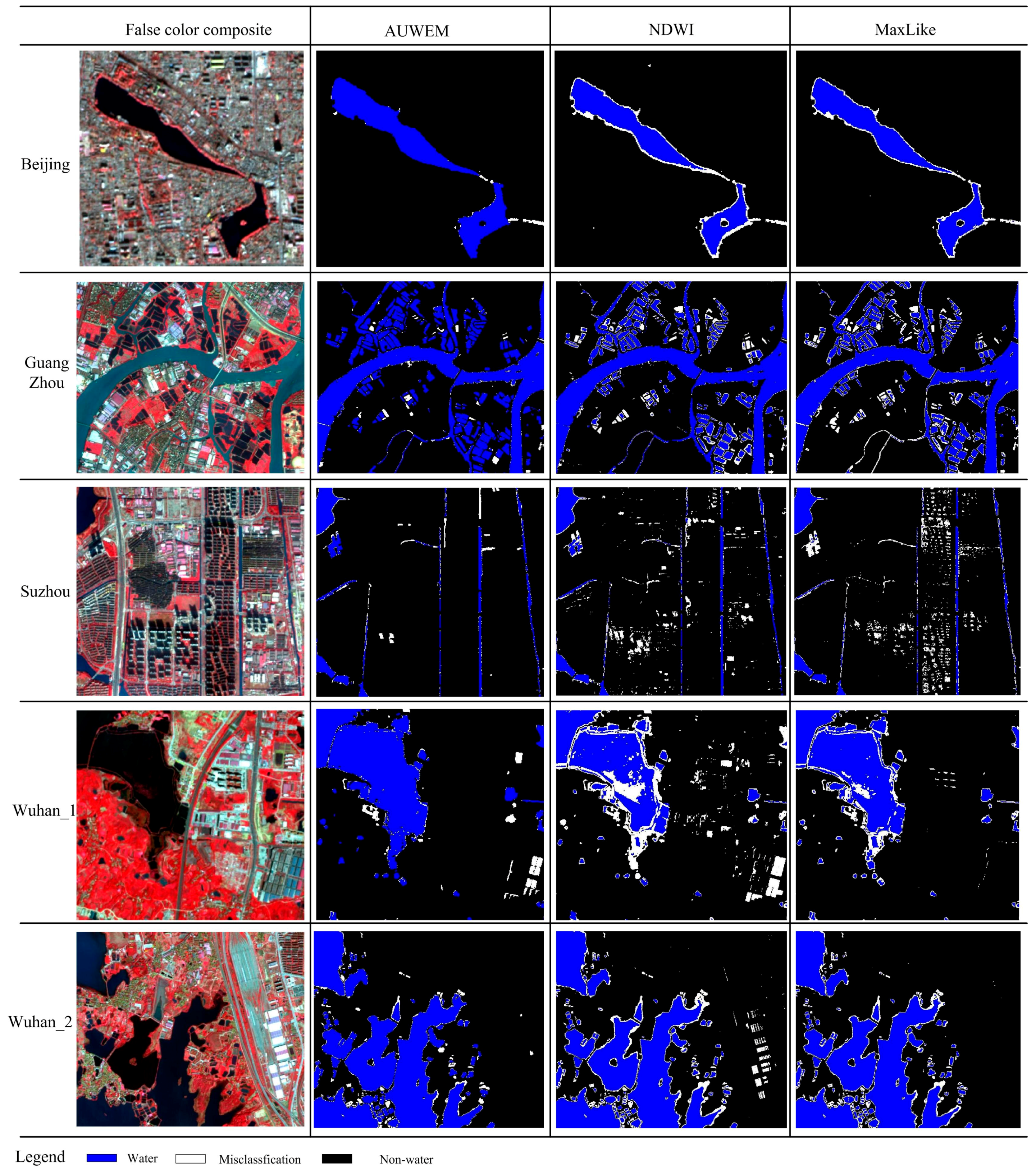
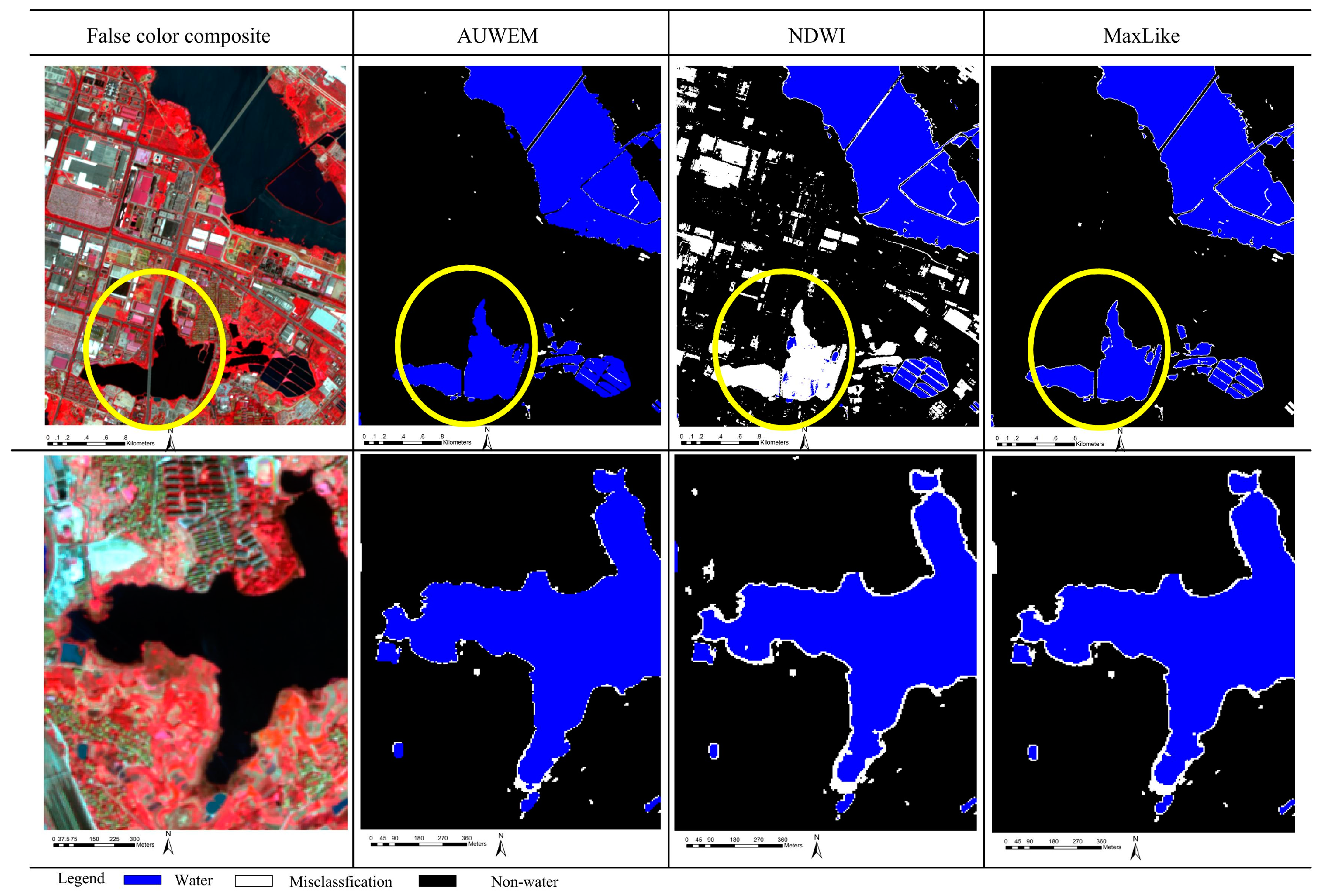
4.1. Water Extraction Maps

To demonstrate the feasibility of the algorithm, we compare the water extraction results generated by using NDWI algorithm and the supervised Maximum Likelihood (MaxLike) classifier was also included in our comparison as the latter one is one of the most widely used methods in land cover classification [16]. Table 4 shows the settings of threshold parameters in different algorithms that are used to extract water from each area. To evaluate the accuracy of the three algorithms, high-resolution fusion imageries are used as the accuracy reference data. We obtain the reference imageries by manually delineating the water edge in fusion imagery, whose information is shown in Table 3. We compare reference imageries with the classification results generated by the three algorithms. For visual interpretation and analysis of classification results generated by different algorithm, the correct classification of water pixels is colored in blue, correct classification of non-water pixels in black. If there are erroneous classifications, corresponding pixels will be highlighted in white.
The experimental results are shown in Figure 7. To facilitate the observation and analysis, we select a small area in yellow rectangular frame from the image, and the classification results are shown in Figure 8. According to the results, the classification accuracy of AUWEM was better than that of NDWI and MaxLike. The AUWEM algorithm excels in classifying mixed pixels of the water edge (judging from the water classification results shown in Beijing, Wuhan_1and Wuhan_2), detecting small pond water compared with NDWI and the MaxLike (judging from classification results shown in Suzhou), and removing shadows of buildings (judging from the classification results shown in Suzhou and Wuhan_2). The NNDWI algorithm is excellent in extracting water bodies that are turbid or whose spectral information is seriously disturbed by vegetation. Therefore, it shows better edge classification results compared with the NDWI algorithm. On the other hand, the classification results of the MaxLike depend on selection of water samples. A limited number of samples will result in unsatisfactory results, especially when the edge pixels are seriously affected by the mixed spectrum. Similarly, small rivers in urban areas are usually flanked with trees, so their spectral information will be seriously disturbed by that of the vegetation. Therefore, the NDWI and MaxLike are inadequate to extract water bodies of small rivers. The Object-Oriented Technology is adopted to differentiate shadows from water bodies by expressing their spectral features, in order to eliminate the influence of high-rise urban buildings on water extraction results.

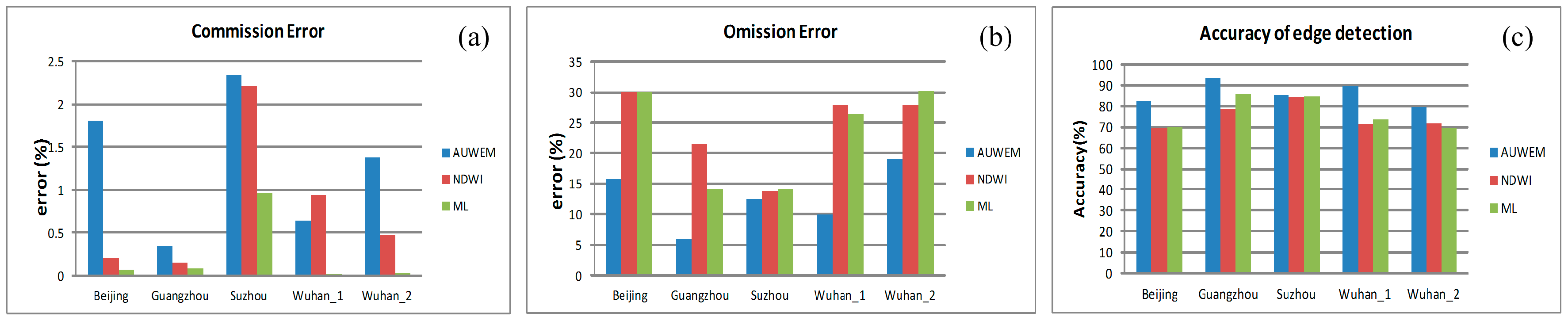
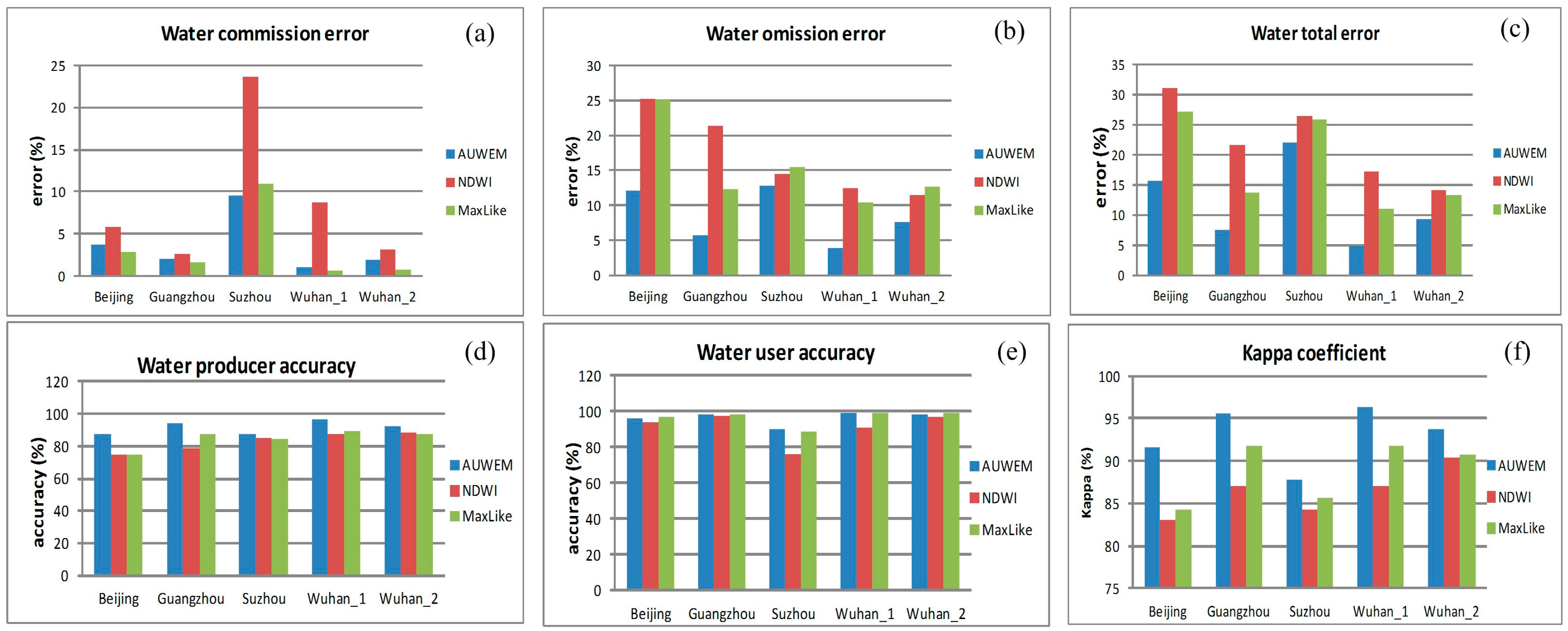
4.2. Water Extraction Accuracy

Accuracy of water extraction can be evaluated by visual interpretation and one-by-one pixel comparison. The visual interpretation has been discussed in Section 4.1. In this section, we will evaluate the classification accuracy by using some quantitative indicators. Table 5 shows the comparison of water classification accuracy among three algorithms in different experimental areas. A statistical analysis of Table 5 indicates that the classification accuracy of AUWEM is greater than that of NDWI and MaxLike. AUWEM algorithm exhibits the greatest classification accuracy in five experimental areas with the average Kappa coefficient of 93%; the NDWI exhibits the lowest classification accuracy with the average Kappa coefficient of about 84.4%; and the MaxLike falls in between, with the average Kappa coefficient of about 88.6%. As shown in the schedule, we use the detailed statistics of the confusion matrix to describe the classification accuracy of the three algorithms in different experimental areas. Among them, Table A1, Table A2, Table A3, Table A4, Table A5, Table A6, Table A7, Table A8, Table A9, Table A10, Table A11, Table A12, Table A13, Table A14 and Table A15 shows the detailed classification accuracy of the three algorithms in different experimental areas.
Figure 9 shows the histogram of water classification accuracy of three different algorithms in the five experimental areas. From the histogram, we can find that the water extraction classification accuracy of AUWEM algorithm is higher than that of NDWI and MaxLike. The commission error of AUWEM is below 5% in most experimental area except in Suzhou (9.5%). The omission error rate of AUWEM is significantly lower than that of NDWI and MaxLike in all the five areas. When both the commission and omission error rates are low, the total error rate will be minimal. From the histogram, we can find that the proposed algorithm exhibits the lowest total error rate, followed by the MaxLike and NDWI. The approximate average total error rates of the three algorithms are about 11.9%, 18.2% and 22.1%, respectively.
In terms of the water classification producer accuracy, the AUWEM algorithm ranks first with the average accuracy of about 91.6%, followed by MaxLike with an average of about 84.8% and NDWI with an average of about 82.9%. In terms of the user accuracy, MaxLike ranks first with the average accuracy of about 96.6%, followed by the proposed algorithm with an average of about 96.4% and NDWI with an average of about 91.2%.

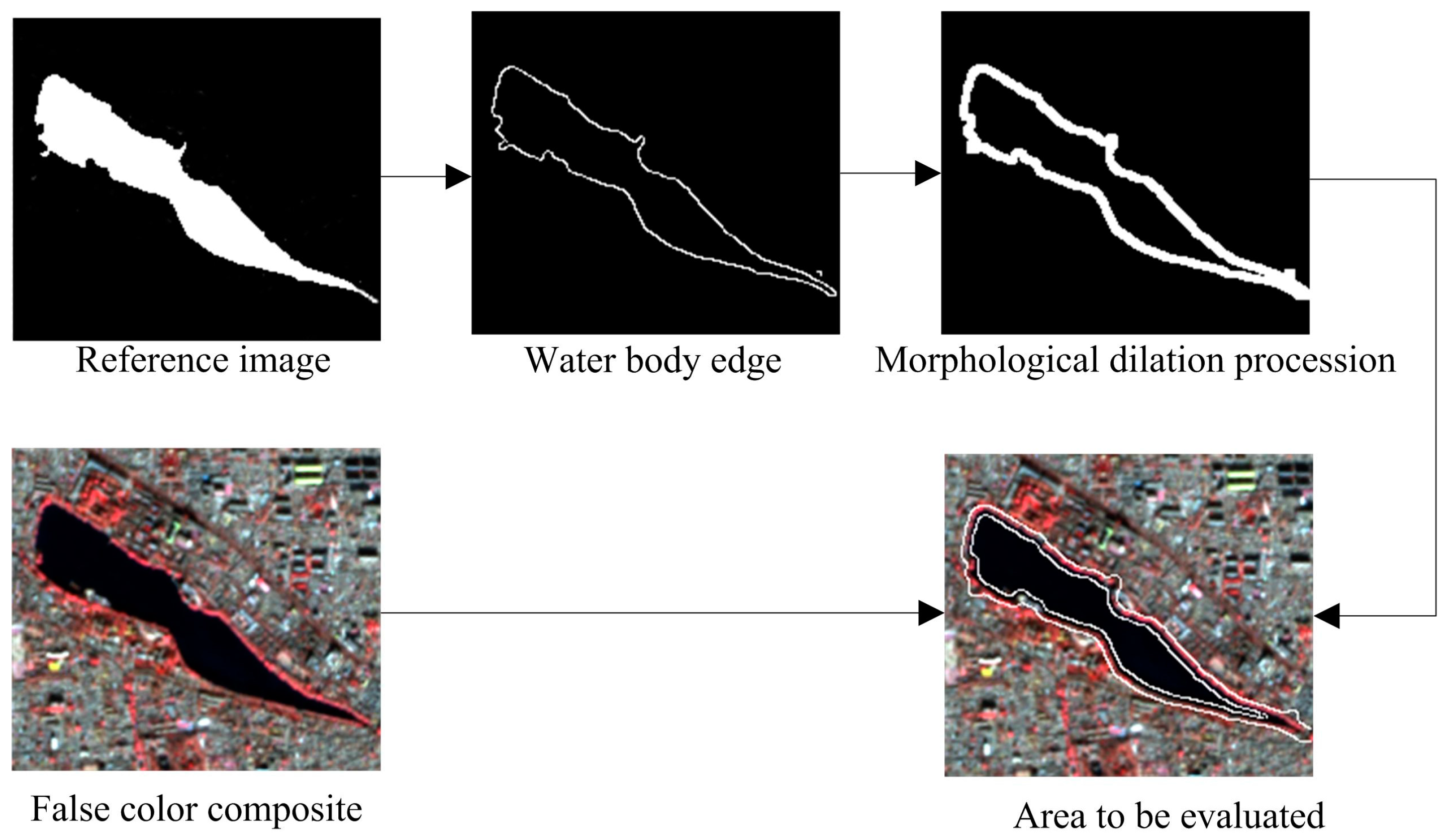
4.3. An Analysis of Water-Edge Pixel Extraction Accuracy

In order to evaluate the edge detection accuracy of the three algorithms more objectively, we design the algorithm below. The steps are as follows:
  • Use the reference image to acquire the water edge by applying the Canny operator.
  • Apply the morphological dilation to the acquired edge to establish a buffer zone centered around the edge with a radius of four pixels.
  • Determine the pixels in the buffer zone. Suppose that the total number of pixels in the buffer zone is N, the number of correctly classified pixels is NR, the number of omitted pixels is No, and the number of commission error is Nc, then:
    A = N R N × 100 %
    E O = N O N × 100 %
    E C = N C N × 100 %
    where A + Eo + Ec = 100%. A indicates the proportion of correctly classified edge pixels (accuracy of edge detection), Eo indicates the proportion of omitted edge pixels (omission error), and Ec is the proportion of commissioned edge pixels (commission error). The edge detection results generated by the approach indicate a comparative rather than absolute conclusion. After all, the reference imageries we use are manually obtained so there will be limitations in visual observations and statistical results are an approximate reflection of the algorithms’ edge extraction accuracy. The process of obtaining the algorithm to acquire the water edge area for evaluation is shown below in Figure 10.
Table 6 showed the statistics about the water edge detection accuracy of above methods in the experimental areas. The statistics include the commission error, omission error and the accuracy of edge detection. Comparison in Figure 11 clearly shows that the edge detection accuracy of the AUWEM algorithm exceeds that of NDWI and MaxLike. The maximum and minimum rates of correct classification of water edge pixels by AUWEM algorithm are 93.7691% (shown in Guangzhou) and 79.5798% (shown in Wuhan_2); the maximum and minimum correct rates of NDWI are 84.0917% (shown in Suzhou) and 69.8310% (shown in Beijing); the maximum and minimum correct rates of MaxLike are 85.8149% (shown in Guangzhou) and 69.7974% (shown in Wuhan_2).

5. Discussion

5.1. Effect of PCA Transformation

By replacing Green in Equation (1) with the first principal component of PCA transformation, we obtain the improved NNDWI2. The NNDWI2 computational result has good resistance to mixed spectral interference, especially when the water bodies are eutrophicated or surrounded by dense vegetation. The pixels of those water bodies exhibit the spectral information of non-water because they are affected and interfered by the spectral information of vegetation like algae, thus their detection will be severely disturbed. According to the classification results shown in Figure 12, the pixels of the water bodies whose spectral information is interfered can be effectively classified in threshold segmentation results of NNDWI2. The number of misclassified pixels generated using the algorithm is less than that generated using NDWI and MaxLike. In addition, the water edge pixels in the images are effectively classified, thus the overall water extraction accuracy is enhanced.

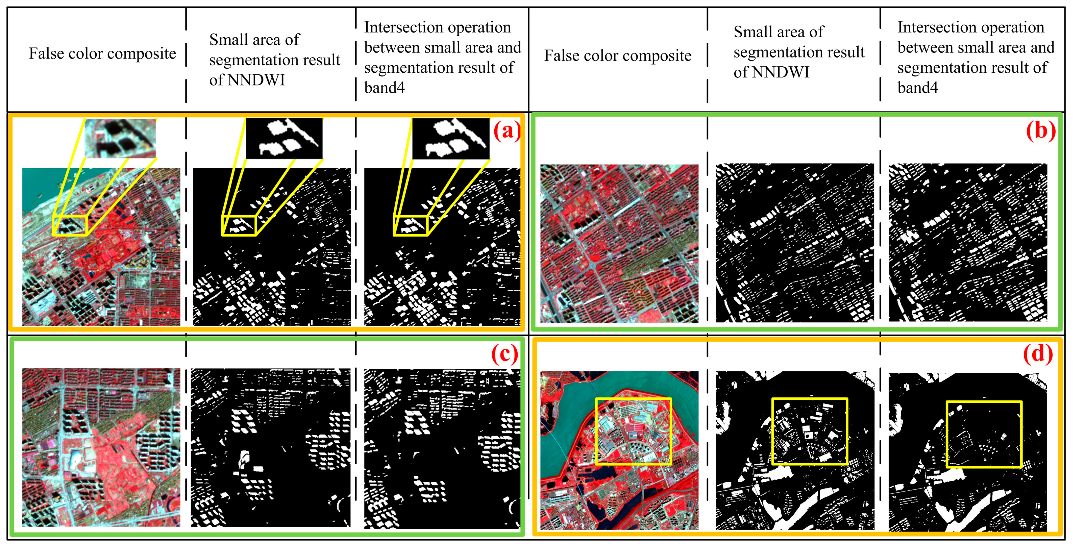
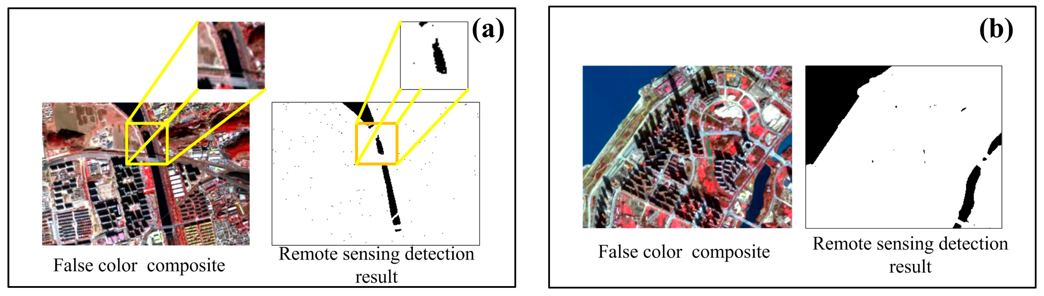
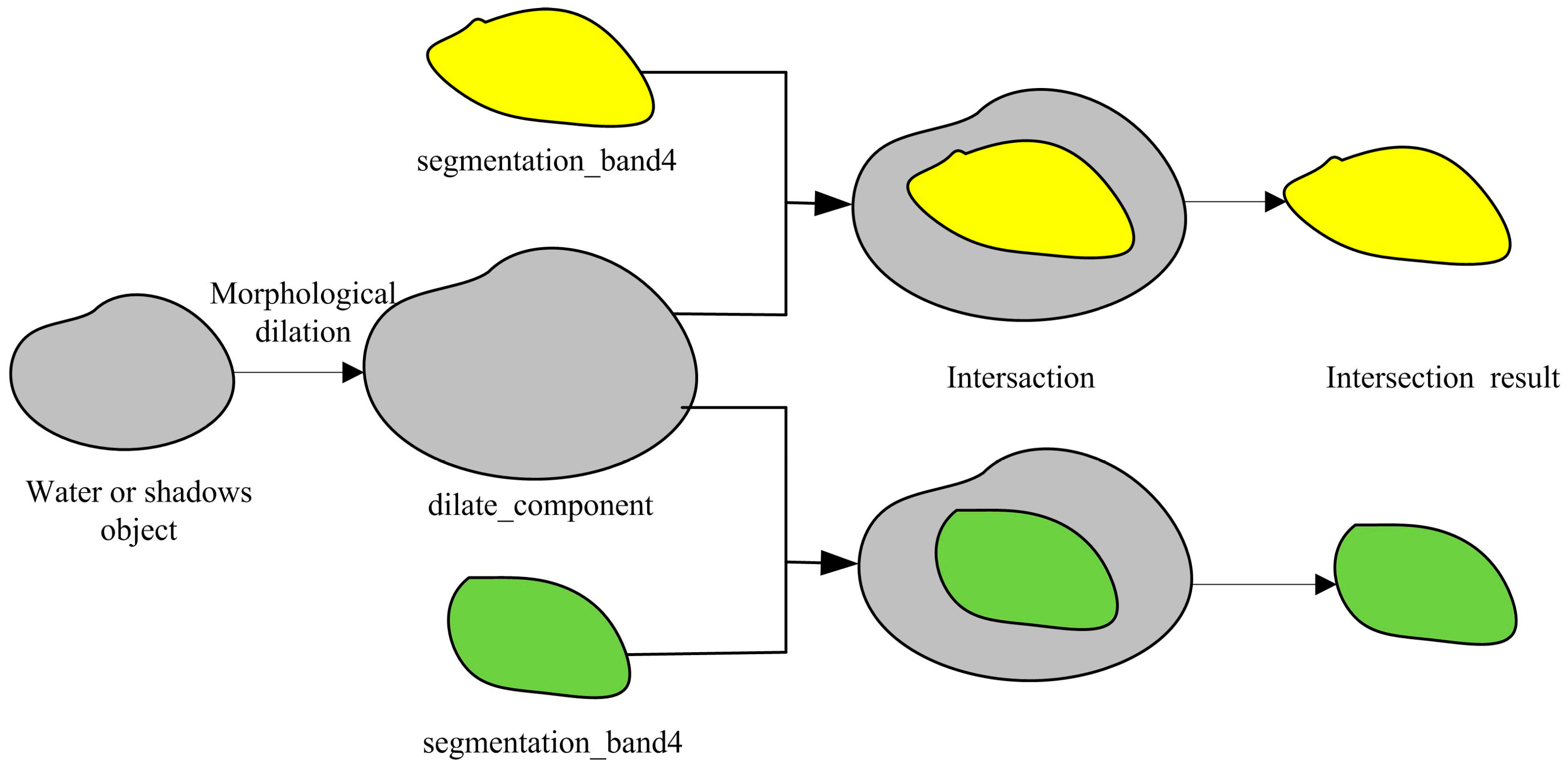
5.2. Effect of Intersection

In Section 3.4.1, we set the constraint on dilation results by intersecting the dilated images and those under threshold segmentation on Band4. However, how many pixels are in the result of the segmentation prior to intersection, and how many pixels are there after the intersection? We choose the following four urban areas for the experiment. The results are shown in the Figure 13. The value changes of water body/shadow pixels before and after computing the intersection are shown in the Table 7. The statistics show that the number of pixels increases after the computation in Figure 13a–c where there are many shadows. After zooming in Figure 13a, we find that after the computation, the building shadows correctly represent the shaded areas. However, the number of pixels is reduced in Figure 13d after the computation, indicating that the computation can result in the removal of error detections generated by the NNDWI algorithm. It can be explained by the experimental results in Figure 14.
As shown in Figure 14, the ground objects in the yellow rectangle are misclassified as water by both NNDWI and NDWI. In fact, these objects are the roof surface of buildings. On the other hand, the objects in this area can be correctly classified by using threshold segmentation result on Band4. After morphological dilation of small-area objects, intersecting it with the images under threshold segmentation on Band4 enables the correction of pixel classification in this area, thus the subsequent classification accuracy of the water bodies will be enhanced.

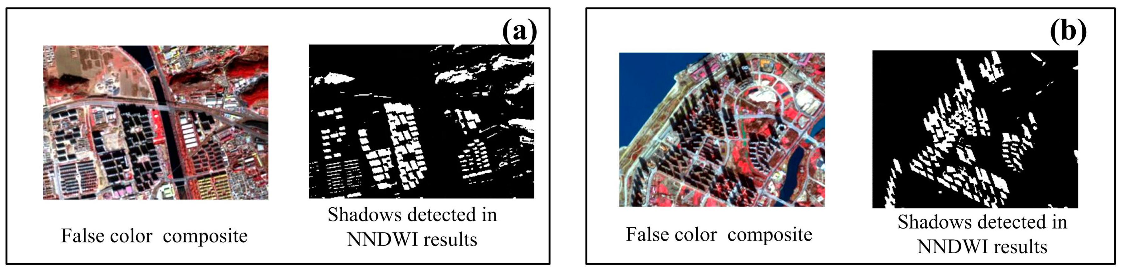
5.3. Shadow Detection Ability of the Shadow Object Description Method

Since the shadow detection algorithm model is established on the premise of extracting water and shadow, we cannot guarantee a sound result by solely relying on it, as shown in Figure 15. The spectral features of the shadows are similar to those of such ground objects as cement surface, soil, vegetation, etc. In our study, we find that the spectral features of such ground objects are presented in the shaded areas. Therefore, it is not ideal to solely use the spectral relation model to detect shadows. Otherwise, almost all of the objects other than water bodies will be detected as shadows. In that case, the imagery is classified into water and non-water areas. However, when zooming in, we find that the water edge detection accuracy is poor; the pixels in water edges cannot be detected properly. On the other hand, when the shadow detection model is used in the NNDWI extraction results, the effect is quite satisfactory, as shown in Figure 16.
From the experiment described above, we can conclude that a combination of the model and the NNDWI extraction results will enable us to effectively detect shadows. When applied solely, the model is not competent in detecting shadows, resulting in misclassification.

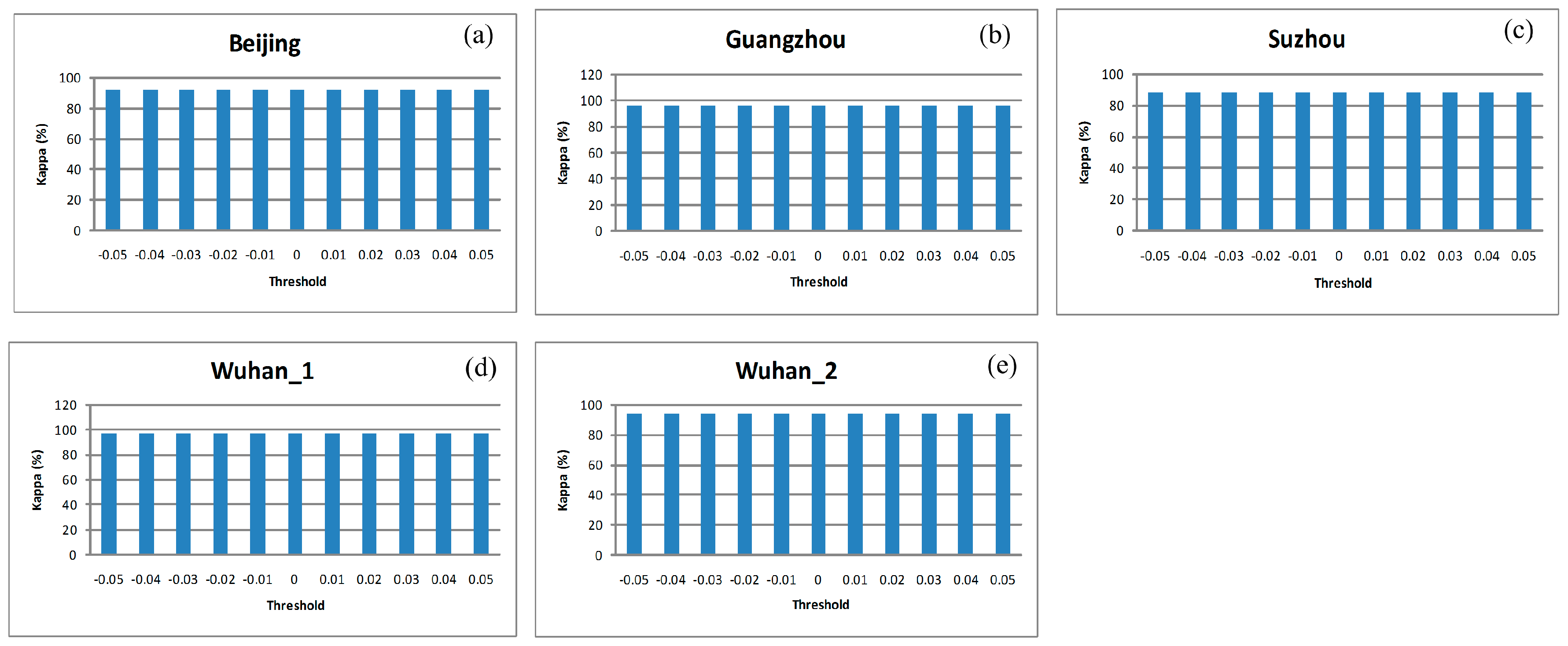
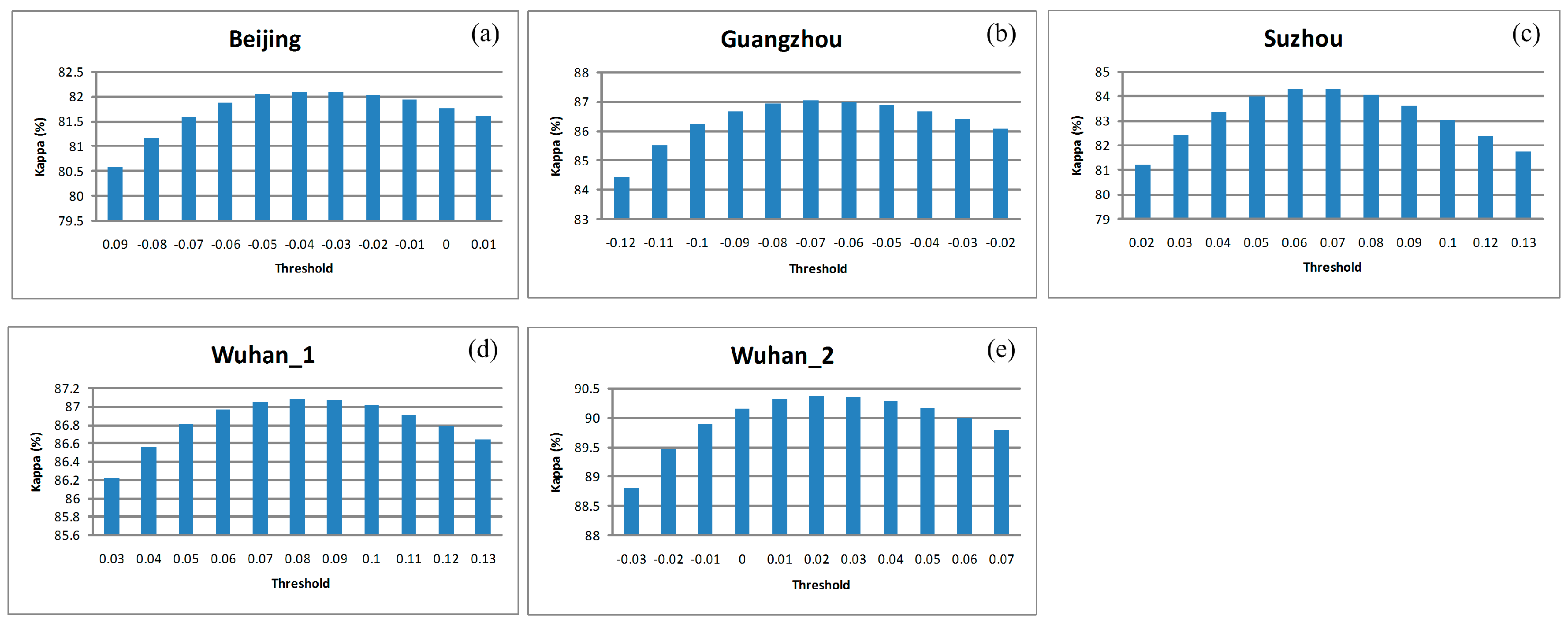
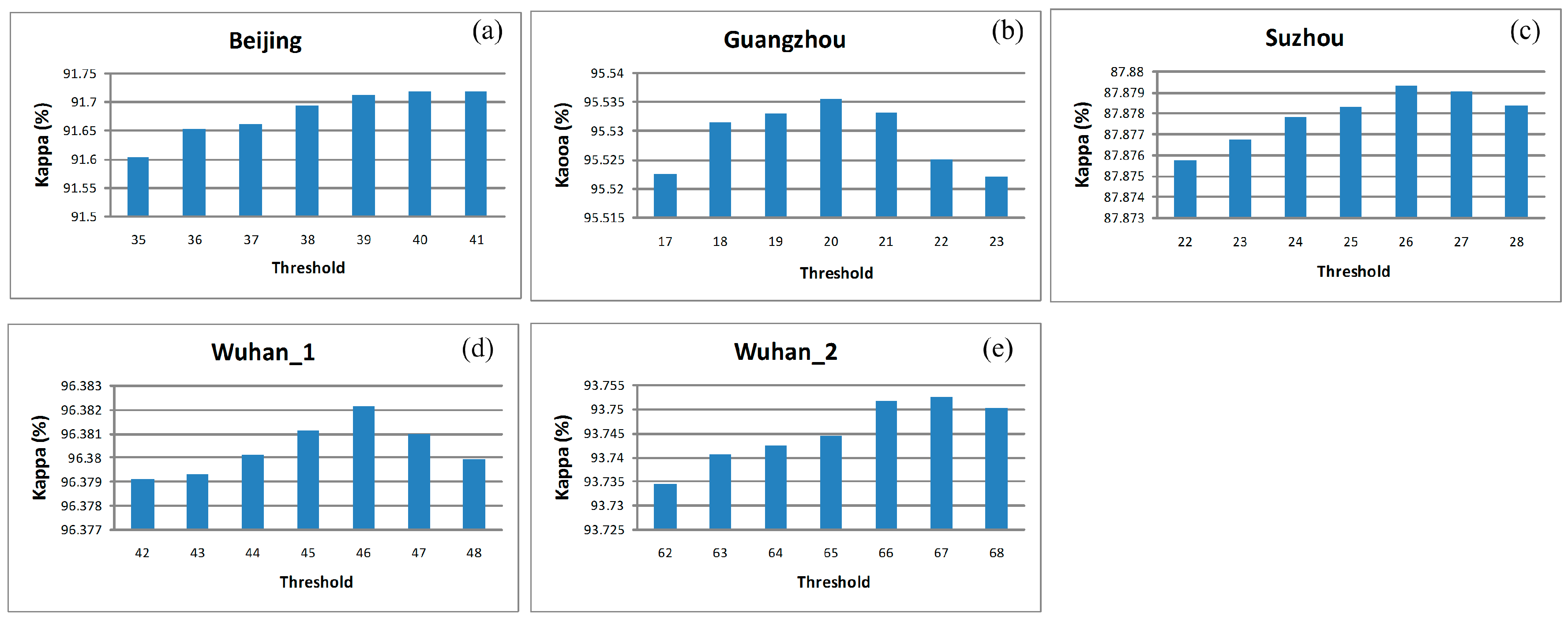
5.4. Threshold Setting and Stability of Algorithm in Correlation Computation

Although there are many problems concerning threshold setting in AUWEM algorithm, it is necessary to set three thresholds, namely NNDWI1, NNDWI2 and Band4 segmentation thresholds. The optimized segmentation threshold value of near-infrared (Band4) is obtained by gray histogram. Before image histogram statistics, we use the Equation (15) to normalize the segmented image pixel value into the range of (0~255). The standardized expression is shown as follows:
y = 255 × ( x x min ) ( x max x min )
where y indicates the standardized value, x indicates all of the pixel values that need to be processed on Band4, xmin indicates the minimum value on Band4, and xmax indicates the maximum value on Band4.
NNDWI1 is more sensitive to the turbid water. When the threshold value is set to 0, the turbid water will be effectively extracted. As for NNDWI2 threshold setting, we can analyze and discuss in detail the following figures. Figure 17a is the false color image for experimental analysis, and Figure 17b shows the pixel value of the first principal component after the PCA transformation on the four bands of the image. It can be seen from the figure that the pixel values of water areas are below 0 in the first principal component (the maximum pixel value is −176.333), while the pixel values of non-water areas are above 0 (the minimum pixel value is 39.8416); in the NNDWI2 calculation results, as shown in Figure 17c, the pixel values of water areas are above 0 (the minimum and maximum pixel values are 2.65607 and 25.17149, respectively), while the pixel values of non-water areas are below 0 (the minimum and maximum pixel values are −6.90065 and −0.44693, respectively). The difference between the minimum value of water areas and the maximum value of non-water areas is 3.103 (in some parts of the image, the actual difference is even greater). Therefore, the optimal segmentation threshold of the images after the computation of NNDWI2 can be set to 0. This is also verified by other experiments, and zero can be used as the best segmentation threshold of NNWI2 index image.
In Figure 18, Figure 19, Figure 20 and Figure 21, we compare the water extraction accuracy among algorithms when the threshold changes. The statistical results show that AUWEM algorithm will not have an obvious impact on classification accuracy when the threshold is within the range of T ± △T. (T is the selected or optimal threshold. In Figure 18, Figure 19 and Figure 20, △T = 0.05, and in Figure 17, △T = 3.) On the other hand, NDWI’s accuracy is greatly affected when the threshold changes. By analyzing the accuracy data of NDWI in Figure 18, we can find that the water extraction accuracy changes drastically when the threshold changes, the variance are 0.4639 (Beijing), 0.7902 (Guangzhou), 1.0588 (Suzhou), 0.2651 (Wuhan_1) and 0.4749 (Wuhan_2). Thus, the changes in threshold affect NDWI’s accuracy (especially in Guangzhou and Suzhou). It shows that the algorithm is unstable. In Figure 19 and Figure 20, we find that when the threshold changes, the accuracy of NNDWI1 and NNDWI2 is almost unchanged. In Figure 21, we find that the accuracy on Band4 is to some extent influenced by the changes in threshold, but such influence is minimal, and the mean square deviation of the accuracy in the experimental areas corroborates with the observation (variance are 0.0433 (Beijing), 0.0056 (Guangzhou), 0.0013 (Suzhou), 0.0011 (Wuhan_1) and 0.0066 (Wuhan_2)). In summary of the statistical analysis of Figure 18, Figure 19, Figure 20 and Figure 21, we can conclude that when the thresholds change, the water extraction accuracy of AUWEM algorithm is more stable than that of NDWI. Even though three threshold values need to be set, the setting is quite simple, so there is no need to consider too many influencing factors.
When the threshold changes, the water extraction accuracy on Band4 is to some extent influenced. Through the experimental analysis, we find that it is mainly caused by the way we compute intersection in Section 3.4.1. The computation results in constraints on the dilation. The related analysis is shown in Figure 22. From the figure, we can find that different threshold segmentation results cover different areas, but the area variation is very small, within the range of T ± △T. The threshold will not impact on the water in terms of covering area and detection, thus barely affecting the detection accuracy.

5.5. Summary

Although results are quite satisfactory in different experimental areas, some issues remain to be considered, such as seasons, the sun’s height angle, components of the atmosphere, and the chemical composition of water bodies. All of these factors have an impact on the reflection features. Different atmospheric correction for subsequent image segmentation threshold may be different, thus affecting the subsequent water detection accuracy; the same atmospheric correction method will exhibit different atmospheric correction accuracy under different weather conditions, especially when there is heavy haze. Heavy haze has been a serious issue in Chinese urban areas during wintertime in recent years. The current atmospheric correction model may not necessarily work well when correcting atmospheric haze. In some areas of the imagery, shadows and water bodies are adjacent. If water body area is large enough, the whole area will be classified as water. Our algorithm is proposed for ZY-3 image data, so whether it has a wider applicability or not needs to be validated by image data from other sources and in different areas. These issues are worth of our follow-up study and verification.

6. Conclusions

We propose a new method for urban water extraction from high-resolution remote sensing images. In order to improve the accuracy of water extraction, we improve the NDWI algorithm and propose two new water indices, namely the NNDWI1 which is sensitive to turbid water, andNNDWI2 which is sensitive to water bodies whose spectral information is interfered by that of vegetation. We superimpose NNDWI1 and NNDWI2 image segmentation results, and then use Object-Oriented Technology to detect and remove shadows in the small areas, in order to obtain the final results of urban water extraction. Our experiments test the accuracy of algorithms in five urban areas. According to the results, the AUWEM algorithm has greater water extraction accuracy compared with NDWI and the MaxLike, with an average Kappa coefficient of 93% and an average total error rate of about 11.9%. In contrast, the average Kappa coefficient and error rate of the MaxLike are about 88.6% and 18.2%, respectively; the average Kappa coefficient and error rate of NDWI is about 86.2% and 22.1%, respectively. In addition, AUWEM exhibits greater accuracy when detecting water edge and small rivers. It can effectively distinguish shadows of high buildings from water bodies to improve the overall accuracy. More importantly, AUWEM has more stable detection accuracy than NDWI has when the threshold changes. It can also be applicable for other water features extraction, and can be applied to monitor and study the changes in water bodies in other places.

Acknowledgments

The authors wish to thank the editors, reviewers, and Yueming Peng’s help. This work was supported by outstanding postgraduate development schemes of School of Geomatics, Liaoning Technical University (YS201503), Key Laboratory Fund Item of Liaoning Provincial Department of Education (LJZS001), Scientific research project of Liaoning Provincial Department of Education (LJYB023) and the National key research and development program of China (2016YFB0501403).

Author Contributions

Jianhua Guo was responsible for the research design, experiment and analysis, and drafting of the manuscript. Fan Yang reviewed the manuscript and was responsible for the analysis of data and main technical guidance. Hai Tan and Jingxue Wang were responsible for drafting and revising the manuscript and took part in the discussion of experiment design. All authors read and approved the manuscript.

Conflicts of Interest

The authors declare no conflict of interest.

Appendix A

Table A1. Statistic results of image water extraction based on maximum likelihood method in Beijing area.
Ground Truth (Pixels)
ClassWaterNo_WaterTotalProduc Accuracy (%)Omission Error (%)
Water34,96111,65746,61874.994625.0054
No_water10612,244,7712,245,83299.95280.0472
Total 36,0222,256,4282,292,450
User Accuracy (%)97.054699.4834
Commission Error (%)2.94540.5166
Overall Accuracy = 99.4452%; Kappa Coefficient = 84.3326%
Table A2. Statistic results of image water extraction based on the NDWI index in Beijing.
Ground Truth (Pixels)
ClassWaterNo_WaterTotalProduc Accuracy (%)Omission Error (%)
Water34,82711,79146,61874.707225.2928
No_water21252,243,7072,245,83299.90540.0946
Total36,9522,255,4982,292,450
User Accuracy (%)94.249399.4772
Commission Error (%)5.75070.5228
Overall Accuracy = 99.3930%; Kappa Coefficient = 83.0431%
Table A3. Statistic results of image water extraction based on AUWEM in Beijing.
Ground Truth (Pixels)
ClassWaterNo_WaterTotalProduc Accuracy (%)Omission Error (%)
Water40,929568946,61887.796612.2034
No_water15712,244,2612,245,83299.93000.0700
Total42,5002,249,9502,292,450
User Accuracy (%)96.303599.7471
Commission Error (%)3.69650.2529
Overall accuracy = 99.6833%; Kappa Coefficient = 91.6924%

Appendix B

Table A4. Statistic results of image water extraction based on maximum likelihood method in Guangzhou.
Ground Truth (Pixels)
ClassWaterNo_WaterTotalProduc Accuracy (%)Omission Error (%)
Water1,212,617169,9761,382,59387.706012.2940
No_water19,1578,988,8859,008,04299.78730.2127
Total1,231,7749,158,86110,390,635
User Accuracy (%)98.444898.1441
Commission Error (%)1.55521.8559
Overall accuracy = 98.1798%; Kappa Coefficient = 91.7285%
Table A5. Statistic results of image water extraction based on the NDWI index in Guangzhou.
Ground Truth (Pixels)
ClassWaterNo_WaterTotalProduc Accuracy (%)Omission Error (%)
Water1,087,494295,0991,382,59378.656121.3439
No_water29,1058,978,9379,008,04299.67690.3231
Total1,116,5999,274,03610,390,635
User Accuracy (%)97.393496.8180
Commission Error (%)2.60663.1820
Overall accuracy = 96.8798%; Kappa Coefficient = 85.2771%
Table A6. Statistic results of image water extraction based on AUWEM in Guangzhou.
Ground Truth (Pixels)
ClassWaterNo_WaterTotalProduc Accuracy (%)Omission Error (%)
Water1,304,00178,5921,382,59394.31565.6844
No_water26,7338,981,3099,008,04299.70320.2968
Total1,330,7349,059,90110,390,635
User Accuracy (%)97.991199.1325
Commission Error (%)2.00890.8675
Overall accuracy = 98.9863%; Kappa Coefficient = 95.5355%

Appendix C

Table A7. Statistic results of image water extraction based on maximum likelihood method in Suzhou.
Ground Truth (Pixels)
ClassWaterNo_WaterTotalProduc Accuracy (%)Omission Error (%)
Water415,71776,225491,94284.505315.4947
No_water50,9485,673,1545,724,10299.10990.8901
Total466,6655,749,3796,216,044
User Accuracy (%)89.082598.6742
Commission Error (%)10.91751.3258
Overall accuracy = 97.9541%; Kappa Coefficient = 85.6260%
Table A8. Statistic results of image water extraction based on the NDWI index in Suzhou.
Ground Truth (Pixels)
ClassWaterNo_WaterTotalProduc Accuracy (%)Omission Error (%)
Water420,72671,216491,94285.523514.4765
No_water130,8845,593,2185,724,10297.71352.2865
Total551,6105,664,4346,216,044
User Accuracy (%)76.272498.7428
Commission Error (%)23.72761.2572
Overall accuracy = 96.7487%; Kappa Coefficient = 78.8652%
Table A9. Statistic results of image water extraction based on AUWEM in Suzhou.
Ground Truth (Pixels)
ClassWaterNo_WaterTotalProduc Accuracy (%)Omission Error (%)
Water429,10162,841491,94287.225912.7741
No_water45,1825,678,9205,724,10299.21070.7893
Total474,2835,741,7616,216,044
User Accuracy (%)90.473698.9055
Commission Error (%)9.52641.0945
Overall accuracy = 98.2622%Kappa Coefficient = 87.8783%

Appendix D

Table A10. Statistic results of image water extraction based on maximum likelihood method in Wuhan_2.
Ground Truth (Pixels)
ClassWaterNo_WaterTotalProduc Accuracy (%)Omission Error (%)
Water1,562,974182,2671,745,24189.556310.4437
No_water92743,905,1303,914,40499.76310.2369
Total1,572,2484,087,3975,659,645
User Accuracy (%)99.410195.5408
Commission Error (%)0.58994.4592
Overall accuracy = 96.6157%; Kappa Coefficient = 91.8418%
Table A11. Statistic results of image water extraction based on the NDWI index in Wuhan_2.
Ground Truth (Pixels)
ClassWaterNo_WaterTotalProduc Accuracy (%)Omission Error (%)
Water1,526,202219,0391,745,24187.449412.5506
No_water146,8673,767,5373,914,40496.24805.4944
Total1,673,0693,986,5765,659,645
User Accuracy (%)91.221794.5056
Commission Error (%)8.77833.7520
Overall accuracy = 93.5348%; Kappa Coefficient = 84.6675%
Table A12. Statistic results of image water extraction based on AUWEM in Wuhan_2.
Ground Truth (Pixels)
ClassWaterNo_WaterTotalProduc Accuracy (%)Omission Error (%)
Water1,676,38768,8541,745,24196.05483.9452
No_water17,8033,896,6013,914,40499.54520.4548
Total1,694,1903,965,4555,659,645
User Accuracy (%)98.949298.2637
Commission Error (%)1.05081.7363
Overall accuracy = 98.4689%; Kappa Coefficient = 96.3811%

Appendix E

Table A13. Statistic results of image water extraction based on maximum likelihood method in Wuhan_3.
Ground Truth (Pixels)
ClassWaterNo_WaterTotal Produc Accuracy (%)Omission Error (%)
Water2,084,870303,3032,388,17387.299812.7002
No_water17,1987,422,6537,439,85199.76880.2312
Total2,102,0687,725,9569,828,024
User Accuracy (%)99.181996.0742
Commission Error (%)0.72013.9258
Overall accuracy = 96.7389%; Kappa Coefficient = 90.7601%
Table A14. Statistic results of image water extraction based on the NDWI index inWuhan_3.
Ground Truth (Pixels)
ClassWaterNo_WaterTotalProduc Accuracy (%)Omission Error (%)
Water2,114,412273,7612,388,17388.536811.4632
No_water68,4787,371,3737,439,85199.07960.9204
Total2,182,8907,645,1349,828,024
User Accuracy (%)96.863096.4191
Commission Error (%)3.13703.5809
Overall accuracy = 96.5177%; Kappa Coefficient = 90.2501%
Table A15. Statistic results of image water extraction based on AUWEM in Wuhan_3.
Ground Truth (Pixels)
ClassWaterNo_WaterTotalProduc Accuracy (%)Omission Error (%)
Water2,207,784180,3892,388,17392.44667.5534
No_water41,3207,398,5317,439,85199.44460.5554
Total2,249,1047,578,9209,828,024
User Accuracy (%)98.162897.6199
Commission Error (%)1.83722.3801
Overall accuracy = 97.7441%; Kappa Coefficient = 93.7445%

References

  1. Stabler, L.B. Management regimes affect woody plant productivity and water use efficiency in an urbandesert ecosystem. Urban Ecosyst. 2008, 11, 197–211. [Google Scholar] [CrossRef]
  2. Mcfeeters, S.K. Using the Normalized Difference Water Index (NDWI) within a Geographic Information System to Detect Swimming Pools for Mosquito Abatement: A Practical Approach. Remote Sens. 2013, 5, 3544–3561. [Google Scholar] [CrossRef]
  3. Zhai, W.; Huang, C. Fast building damage mapping using a single post-earthquake PolSAR image: A case study of the 2010 Yushu earthquake. Earth Planets Space 2016, 68, 1–12. [Google Scholar] [CrossRef]
  4. Raju, P.L.N.; Sarma, K.K.; Barman, D.; Handique, B.K.; Chutia, D.; Kundu, S.S.; Das, R.; Chakraborty, K.; Das, R.; Goswami, J.; et al. Operational remote sensing services in north eastern region of India for natural resources management, early warning for disaster risk reduction and dissemination of information and services. ISPRS—Int. Arch. Photogramm. Remote Sens. Spat. Inform. Sci. 2016, XLI-B4, 767–775. [Google Scholar] [CrossRef]
  5. Muriithi, F.K. Land use and land cover (LULC) changes in semi-arid sub-watersheds of Laikipia and Athi River basins, Kenya, as influenced by expanding intensive commercial horticulture. Remote Sens. Appl. Soc. Environ. 2016, 3, 73–88. [Google Scholar] [CrossRef]
  6. Byun, Y.; Han, Y.; Chae, T. Image fusion-based change detection for flood extent extraction using bi-temporal very high-resolution satellite images. Remote Sens. 2015, 7, 10347–10363. [Google Scholar] [CrossRef]
  7. Kang, L.; Zhang, S.; Ding, Y.; He, X. Extraction and preference ordering of multireservoir water supply rules in dry years. Water 2016, 8, 28. [Google Scholar] [CrossRef]
  8. Katz, D. Undermining demand management with supply management: Moral hazard in Israeli water policies. Water 2016, 8, 159. [Google Scholar] [CrossRef]
  9. Deus, D.; Gloaguen, R. Remote sensing analysis of lake dynamics in semi-arid regions: Implication for water resource management. Lake Manyara, east African Rift, northern Tanzania. Water 2013, 5, 698–727. [Google Scholar] [CrossRef]
  10. Zhai, K.; Xiaoqing, W.U.; Qin, Y.; Du, P. Comparison of surface water extraction performances of different classic water indices using OLI and TM imageries in different situations. Geo-Spat. Inform. Sci. 2015, 18, 32–42. [Google Scholar] [CrossRef]
  11. Gautam, V.K.; Gaurav, P.K.; Murugan, P.; Annadurai, M. Assessment of surface water dynamics in Bangalore using WRI, NDWI, MNDWI, supervised classification and K-T transformation. Aquat. Procedia 2015, 4, 739–746. [Google Scholar] [CrossRef]
  12. Bryant, R.G.; Rainey, M.P. Investigation of flood inundation on playas within the Zone of Chotts, using a time-series of AVHRR. Remote Sens. Environ. 2002, 82, 360–375. [Google Scholar] [CrossRef]
  13. Sun, F.; Sun, W.; Chen, J.; Gong, P. Comparison and improvement of methods for identifying water bodies in remotely sensed imagery. Int. J. Remote Sens. 2012, 33, 6854–6875. [Google Scholar] [CrossRef]
  14. Mcfeeters, S.K. The use of the Normalized Difference Water Index (NDWI) in the delineation of open water features. Int. J. Remote Sens. 1996, 17, 1425–1432. [Google Scholar] [CrossRef]
  15. Xu, H. Modification of normalized difference water index (NDWI) to enhance open water features in remotely sensed imagery. Int. J. Remote Sens. 2006, 27, 3025–3033. [Google Scholar] [CrossRef]
  16. Feyisa, G.L.; Meilby, H.; Fensholt, R.; Proud, S.R. Automated Water Extraction Index: A new technique for surface water mapping using Landsat imagery. Remote Sens. Environ. 2014, 140, 23–35. [Google Scholar] [CrossRef]
  17. Rogers, A.S.; Kearney, M.S. Reducing signature variability in unmixing coastal marsh Thematic Mapper scenes using spectral indices. Int. J. Remote Sens. 2004, 25, 2317–2335. [Google Scholar] [CrossRef]
  18. Lira, J. Segmentation and morphology of open water bodies from multispectral images. Int. J. Remote Sens. 2006, 27, 4015–4038. [Google Scholar] [CrossRef]
  19. Lv, W.; Yu, Q.; Yu, W. Water Extraction in SAR Images Using GLCM and Support Vector Machine. In Proceedings of the IEEE 10th International Conference on Signal Processing Proceedings, Beijing, China, 24–28 October 2010.
  20. Wendleder, A.; Breunig, M.; Martin, K.; Wessel, B.; Roth, A. Water body detection from TanDEM-X data: Concept and first evaluation of an accurate water indication mask. Soc. Sci. Electron. Publ. 2011, 25, 3779–3782. [Google Scholar]
  21. Wendleder, A.; Wessel, B.; Roth, A.; Breunig, M.; Martin, K.; Wagenbrenner, S. TanDEM-X water indication mask: Generation and first evaluation results. IEEE J. Sel. Top. Appl. Earth Obs. Remote Sens. 2012, 6, 1–9. [Google Scholar] [CrossRef] [Green Version]
  22. Wang, Y.; Ruan, R.; She, Y.; Yan, M. Extraction of water information based on RADARSAT SAR and Landsat ETM+. Procedia Environ. Sci. 2011, 10, 2301–2306. [Google Scholar] [CrossRef]
  23. Wang, K.; Trinder, J.C. Applied Watershed Segmentation Algorithm for Water Body Extraction in Airborne SAR Image. In Proceedings of the European Conference on Synthetic Aperture Radar, Aachen, Germany, 2–4 June 2014.
  24. Ahtonen, P.; Hallikainen, M. Automatic Detection of Water Bodies from Spaceborne SAR Images. In Proceedings of the 2005 IEEE International on Geoscience and Remote Sensing Symposium, IGARSS ‘05, Seoul, Korea, 25–29 July 2005.
  25. Li, B.; Zhang, H.; Xu, F. Water Extraction in High Resolution Remote Sensing Image Based on Hierarchical Spectrum and Shape Features. In Proceedings of the 35th International Symposium on Remote Sensing of Environment (ISRSE35), Beijing, China, 22–26 April 2013.
  26. Deng, Y.; Zhang, H.; Wang, C.; Liu, M. Object-Oriented Water Extraction of PolSAR Image Based on Target Decomposition. In Proceedings of the 2015 IEEE 5th Asia-Pacific Conference on Synthetic Aperture Radar (APSAR), Singapore, 1–4 September 2015.
  27. Jiang, H.; Feng, M.; Zhu, Y.; Lu, N.; Huang, J.; Xiao, T. An automated method for extracting rivers and lakes from Landsat imagery. Remote Sens. 2014, 6, 5067–5089. [Google Scholar] [CrossRef]
  28. Steele, M.K.; Heffernan, J.B. Morphological characteristics of urban water bodies: Mechanisms of change and implications for ecosystem function. Ecol. Appl. 2014, 24, 1070–1084. [Google Scholar] [CrossRef] [PubMed]
  29. Yu, X.; Li, B.; Shao, J.; Zhou, J.; Duan, H. Land Cover Change Detection of Ezhou Huarong District Based on Multi-Temporal ZY-3 Satellite Images. In Proceedings of the 2015 IEEE 23rd International Conference on Geoinformatics, Wuhan, China, 19–21 June 2015.
  30. Dong, Y.; Chen, W.; Chang, H.; Zhang, Y.; Feng, R.; Meng, L. Assessment of orthoimage and DEM derived from ZY-3 stereo image in Northeastern China. Surv. Rev. 2015, 48, 247–257. [Google Scholar] [CrossRef]
  31. Yao, F.; Wang, C.; Dong, D.; Luo, J.; Shen, Z.; Yang, K. High-resolution mapping of urban surface water using ZY-3 multi-spectral imagery. Remote Sens. 2015, 7, 12336–12355. [Google Scholar] [CrossRef]
  32. Su, N.; Zhang, Y.; Tian, S.; Yan, Y.; Miao, X. Shadow detection and removal for occluded object information recovery in urban high-resolution panchromatic satellite images. IEEE J. Sel. Top. Appl. Earth Obs. Remote Sens. 2016, 9, 1–15. [Google Scholar] [CrossRef]
  33. Li, Y.; Gong, P.; Sasagawa, T. Integrated shadow removal based on photogrammetry and image analysis. Int. J. Remote Sens. 2005, 26, 3911–3929. [Google Scholar] [CrossRef]
  34. Zhou, W.; Huang, G.; Troy, A.; Cadenasso, M.L. Object-based land cover classification of shaded areas in high spatial resolution imagery of urban areas: A comparison study. Remote Sens. Environ. 2009, 113, 1769–1777. [Google Scholar] [CrossRef]
  35. Xie, J.; Zhang, L.; You, J.; Shiu, S. Effective texture classification by texton encoding induced statistical features. Pattern Recognit. 2014, 48, 447–457. [Google Scholar] [CrossRef]
  36. Lizarazo, I. SVM-based segmentation and classification of remotely sensed data. Int. J. Remote Sens. 2008, 29, 7277–7283. [Google Scholar] [CrossRef]
  37. Huang, X.; Zhang, L. Morphological building/shadow index for building extraction from high-resolution imagery over urban areas. IEEE J. Sel. Top. Appl. Earth Obs. Remote Sens. 2012, 5, 161–172. [Google Scholar] [CrossRef]
  38. Xie, C.; Huang, X.; Zeng, W.; Fang, X. A novel water index for urban high-resolution eight-band WorldView-2 imagery. Int. J. Digit. Earth 2016, 9, 925–941. [Google Scholar] [CrossRef]
  39. Sivanpilla, R.; Miller, S.N. Improvements in mapping water bodies using ASTER data. Ecol. Inform. 2010, 5, 73–78. [Google Scholar] [CrossRef]
  40. Nazeer, M.; Nichol, J.E.; Yung, Y.K. Evaluation of atmospheric correction models and Landsat surface reflectance product in an urban coastal environment. Int. J. Remote Sens. 2014, 35, 6271–6291. [Google Scholar] [CrossRef]
  41. Pechenizkiy, M.; Tsymbal, A.; Puuronen, S. PCA-based feature transformation for classification: Issues in medical diagnostics. Proc. IEEE Symp. Comput. Based Med. Syst. 2004, 1, 535–540. [Google Scholar]
  42. Heijmans, H.J.A.M.; Ronse, C. The algebraic basis of mathematical morphology I. Dilations and erosions. Comput. Vis. Graph. Image Process. 1990, 50, 245–295. [Google Scholar] [CrossRef]
Figure 1. Manually drawn referential imagery.
Water 09 00144 g001
Figure 2. Comparison of ground objects’ spectral curves before and after the atmospheric correction.
Water 09 00144 g002
Figure 3. Different water extraction results generated by NNDWI1, NNDWI2 and NNDWI, respectively.
Water 09 00144 g003
Figure 4. Diagram of dilation constraint.
Water 09 00144 g004
Figure 5. The spectral feature curves of the shadow-area pixels: (ae) typical spectral curves of five types of pixels.
Water 09 00144 g005
Figure 6. The overall flowchart of AUWEM.
Water 09 00144 g006
Figure 7. Comparison of water extraction results of three algorithms in different experimental areas.
Water 09 00144 g007
Figure 8. Comparison of water classification results among different algorithms in local areas (a small area in yellow rectangular frame from the image of Figure 8).
Water 09 00144 g008
Figure 9. A comparison of classification accuracy among different algorithms in five experimental areas. (a) water commission error; (b) Water omission error; (c) Water total error; (d) Water producer accuracy; (e) Water user accuracy; (f) Kappa coefficient.
Water 09 00144 g009
Figure 10. Process of acquiring water edge area for evaluation. Edge of the reference images are extracted and processed by morphological dilation to acquire the water edge for evaluation.
Water 09 00144 g010
Figure 11. Comparison of water edge detection accuracy among different algorithms in five experimental areas. (a) Commission Error; (b) Omission Error; (c) Accuracy of edge detection.
Water 09 00144 g011
Figure 12. Comparison of results of classifying pixels of spectrally contaminated water bodies among different algorithms. The yellow circle indicates an area clearly undetected by the NDWI algorithm. The water body in this area is eutrophicated with a lot of algal vegetation that affects its spectral information, making it hard for the NDWI to detect.
Water 09 00144 g012
Figure 13. Intersection operation results. (a) First experimental results; (b) Second experimental results; (c) Third experimental results; (d) Fourth experimental results.
Water 09 00144 g013
Figure 14. Comparison between intersection result and NDWI result.
Water 09 00144 g014
Figure 15. Shadow detection results generated when solely applying the model. (a) First experimental results; (b) Second experimental results.
Water 09 00144 g015
Figure 16. The shadow detection results generated when combining the model with the NNDWI extraction results. (a) First experimental results; (b) Second experimental results.
Water 09 00144 g016
Figure 17. The different index of pixels after the PCA transformation, NNDWI2 and NDWI, respectively.
Water 09 00144 g017
Figure 18. A comparison among changes of NDWI’s water extraction accuracy when the threshold changes. (a) Water extraction accuracy of Beijing; (b) Water extraction accuracy of Guangzhou; (c) Water extraction accuracy of Suzhou; (d) Water extraction accuracy of Wuhan_1; (e) Water extraction accuracy of Wuhan_2.
Water 09 00144 g018
Figure 19. The changes in NNDWI1 when the threshold changes and Band4 and NNDWI2 remain unchanged. (a) Water extraction accuracy of Beijing; (b) Water extraction accuracy of Guangzhou; (c) Water extraction accuracy of Suzhou; (d) Water extraction accuracy of Wuhan_1; (e) Water extraction accuracy of Wuhan_2.
Water 09 00144 g019
Figure 20. The changes in NNDWI2 when the threshold changes and Band4 and NNDWI1 remain unchanged. (a) Water extraction accuracy of Beijing; (b) Water extraction accuracy of Guangzhou; (c) Water extraction accuracy of Suzhou; (d) Water extraction accuracy of Wuhan_1; (e) Water extraction accuracy of Wuhan_2.
Water 09 00144 g020
Figure 21. The changes in Band4 when the threshold changes and NNDWI1 and NNDWI2 remain unchanged. (a) Water extraction accuracy of Beijing; (b) Water extraction accuracy of Guangzhou; (c) Water extraction accuracy of Suzhou; (d) Water extraction accuracy of Wuhan_1; (e) Water extraction accuracy of Wuhan_2.
Water 09 00144 g021
Figure 22. Comparison of intersection on Band4 under different thresholds as constraint. The yellow segmentation area is larger than the green one, so according to the results in the figure, after the intersection there will be water body or shadow objects that cover different areas and are to be detected.
Water 09 00144 g022
Table 1. Description of studied areas.
City’s Name and LocationArea Coverage (Pixels)Water Body TypeTopographyClimateColor Infrared Composite (4/3/2 Band Combination)
Beijing (39.9° N, 116.3° E)1479 × 1550 (77.1 km2)Rivers
Polluted lakes
Clear lake
PlainWarm temperate semi humid continental monsoon climate Water 09 00144 i001
Guangzhou (23° N, 113.6° E)2351 × 2644 (209.1 km2)Rivers
Ponds
Polluted lakes
Clear lake
Basin, plainTypical monsoon climate in South Asia Water 09 00144 i002
Suzhou (31.2° N, 120.5° E)2351 × 2644 (209.1 km2)Rivers
Ponds
Polluted lakes
Clear lake
Basin, plain, hills.Subtropical humid monsoon climate Water 09 00144 i003
Wuhan_1 (30.5° N, 114.3° E)2245 × 2521 (190.4 km2)Rivers
Ponds
Large polluted lakes
Large clear lakes
Basin, plain, hills.Subtropical humid monsoon climate Water 09 00144 i004
Wuhan_2 (30.5° N, 114.3° E)2894 × 3396 (330.6 km2)Rivers
Ponds
Large polluted lakes
Large clear lakes
Basin, plain, hills.Subtropical humid monsoon climate Water 09 00144 i005
Table 2. ZY-3 satellite Parameters.
ItemContents
Camera modelPanchromatic orthographic; Panchromatic front-view and rear-view; multi-spectral orthographic
ResolutionSub-satellite points full-color: 2.1 m; front- and rear-view 22° full color: 3.6 m; sub-satellite points multi-spectral: 5.8 m
WavelengthPanchromatic: 450 nm–800 nm Multi-spectral: Band1 (450 nm–520 nm); Band2 (520 nm–590 nm) Band3 (630 nm–690 nm); Band4 (770 nm–890 nm)
WidthSub-satellite points Panchromatic: 50 km, single-view 2500 km2; Sub-satellite points multi-spectral: 52 km, single-view 2704 km2
Revisit cycle5 days
Daily image acquisitionPanchromatic: nearly 1,000,000 km2/day; Fusion: nearly 1,000,000 km2/day
Table 3. Description of ZY-3 scenes.
Test SiteZY-3 Scenes
Acquisition DatePathRow
Beijing28 November 2013002125
Guangzhou20 October 2013895167
Suzhou17 December 2015882147
Wuhan_124 July 2016001149
Wuhan_228 March 2016897148
Table 4. Threshold setting of the three algorithms in different experimental areas. Among them, T, T1, T2 and T3 are the threshold of NDWI, NNDWI1, NNDWI2 and Band4, respectively.
MethodThreshold
BeijingGuangzhouSuzhouWuhan_1Wuhan_2
AUWEMT1 = 0, T2 = 0, T3 = 38T1 = 0, T2 = 0, T3 = 20T1 = 0, T2 = 0, T3 = 25T1 = 0, T2 = 0, T3 = 45T1 = 0, T2 = 0, T3 = 65
NDWIT = −0.04T = −0.07T = 0.07T = 0.08T = 0.02
MaxLike-----
Table 5. The statistics of accuracy of three algorithms in different experimental areas.
Classification AlgorithmBeijing (1479 × 1550)Guangzhou (2973 × 3495)Suzhou (2351 × 2644)Wuhan_1 (2245 × 2521)Wuhan_2 (2894 × 3396)
Kappa (%)Kappa (%)Kappa (%)Kappa (%)Kappa (%)
AUWEM91.692495.535587.878396.381193.7445
NDWI83.043185.277178.865284.667590.2501
MaxLike84.332691.728585.626091.841890.7601
Table 6. Statistics about water edge detection accuracy of different algorithms in five experimental areas.
SiteMethodCommission Error (%)Omission Error (%)A (%)
BeijingAUWEM1.803215.844682.3522
NDWI0.204229.964869.8310
MaxLike0.073829.974769.9515
GuangzhouAUWEM0.34175.889293.7691
NDWI0.143821.411478.4448
MaxLike0.083314.101985.8149
SuzhouAUWEM2.345512.579185.0755
NDWI2.214013.694384.0917
MaxLike0.964914.215584.8196
Wuhan_1AUWEM0.64229.892589.4653
NDWI0.945227.849471.2054
MaxLike0.021126.391973.5870
Wuhan_2AUWEM1.382719.037579.5798
NDWI0.474327.840271.6855
MaxLike0.033530.169169.7974
Table 7. Statistics shows the changes of the number of water body/shadow pixels before and after the computation of intersection. Nb represents the number of pixels of water/shadow before the intersection, and Na represents the number of pixels of water/shadow after the intersection.
Image NameImage SizeNbNaNb-Na
a361 × 36111,88315,8884005
b327 × 33512,33617,6305294
c299 × 319992312,2182295
d677 × 76276,93257,389−19,543

