
Variability in the Water Footprint of Arable Crop Production across European Regions

 ,
,  , ,
, , 


Abstract
:1. Introduction
2. Materials and Methods
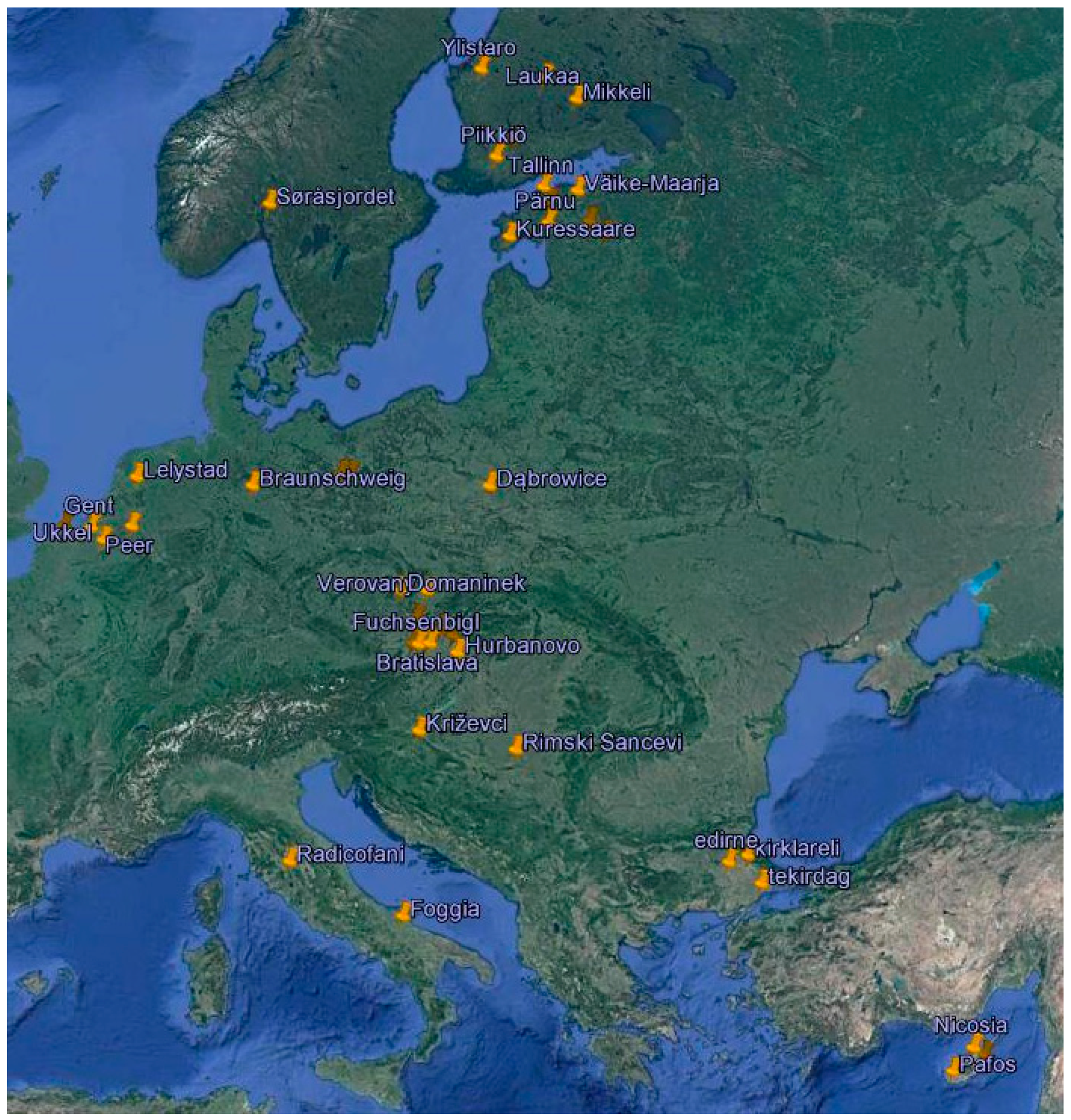
2.1. Data
2.2. Crop Water Use
2.3. Water Footprint Calculations
2.4. Yield Statistics
2.5. Statistical Analysis
3. Results
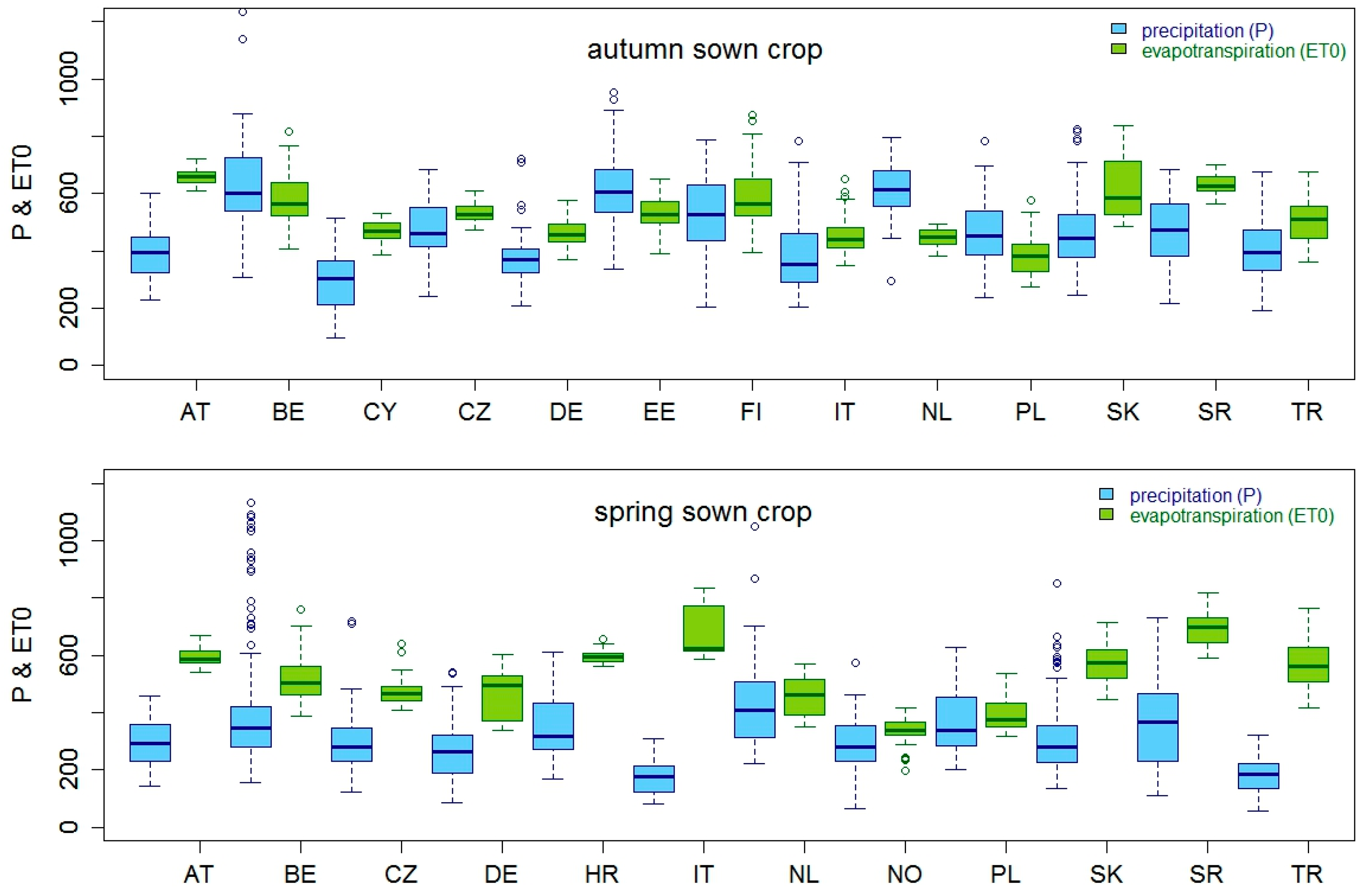
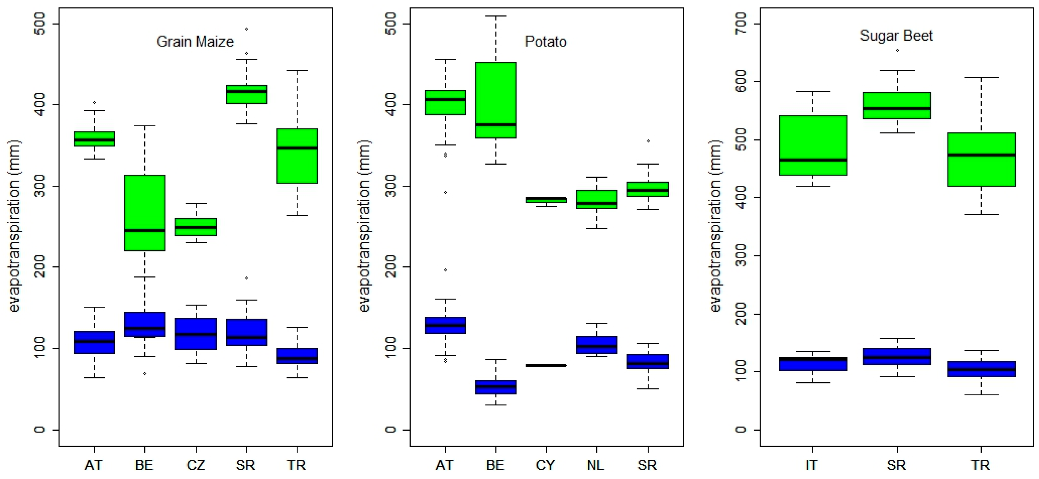
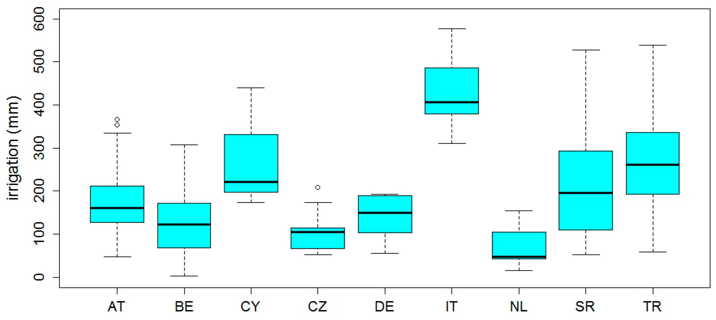
3.1. Water Balance
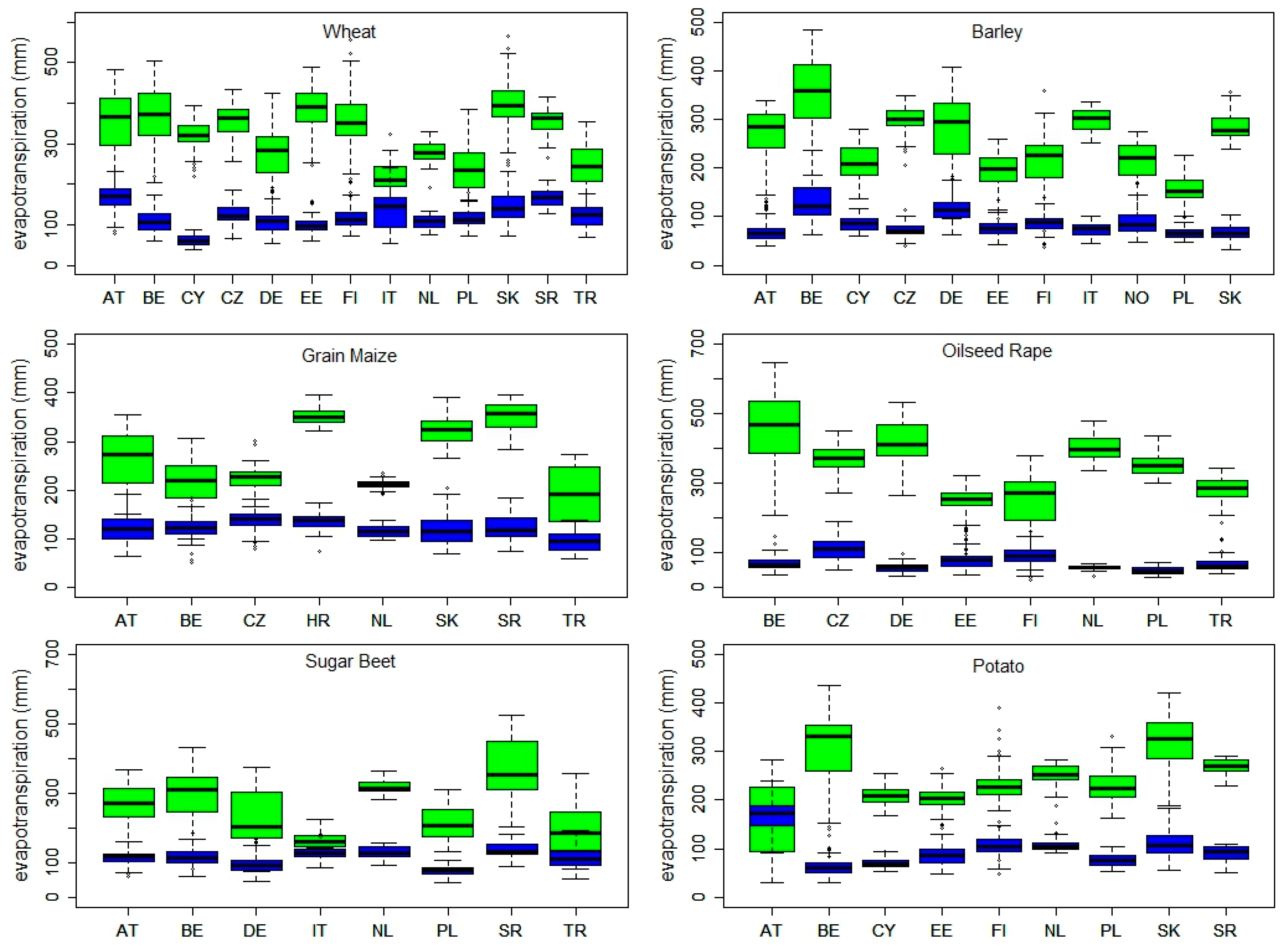
3.2. Soil Evaporation and Crop Transpiration
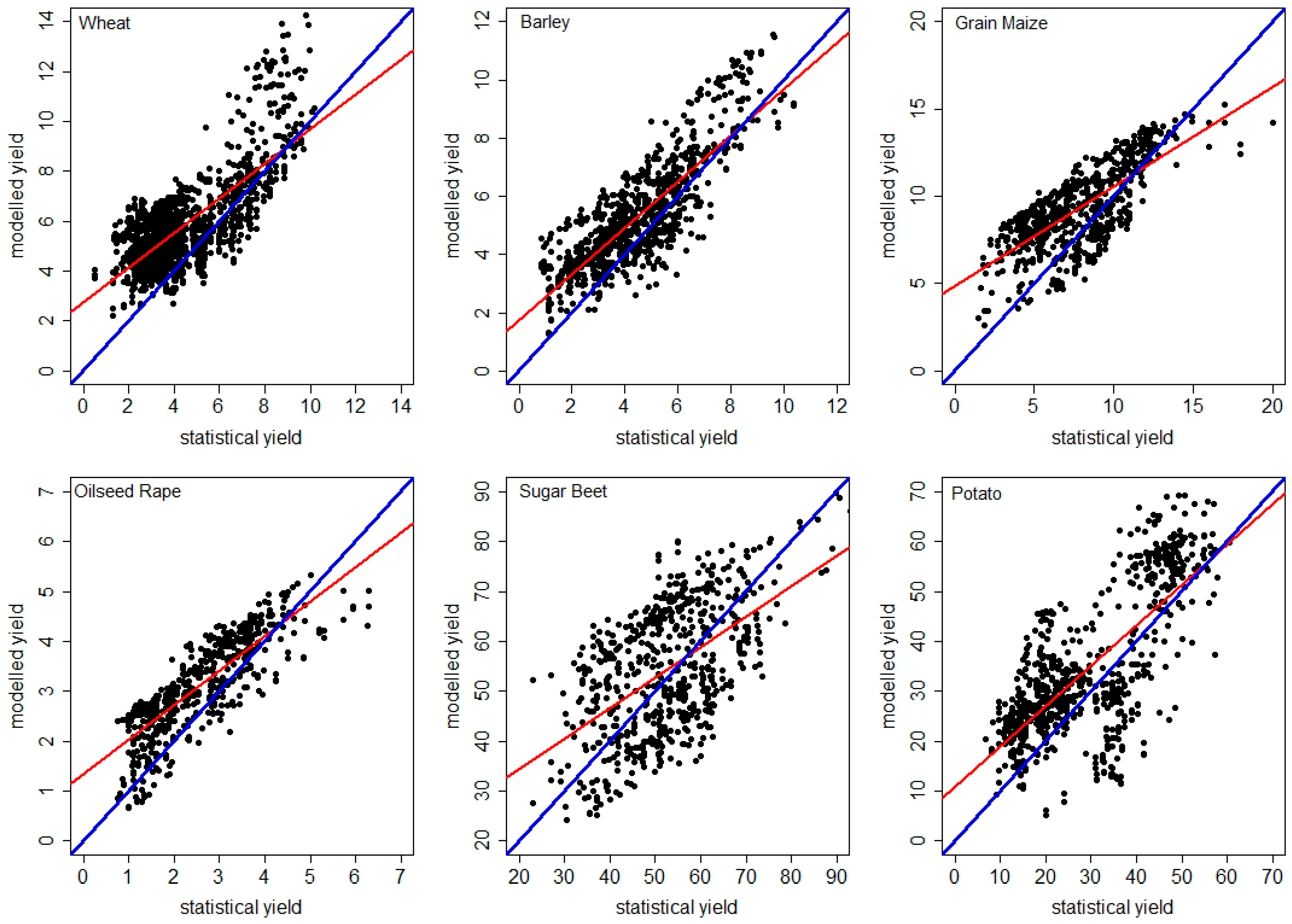
3.3. Biomass and Yield
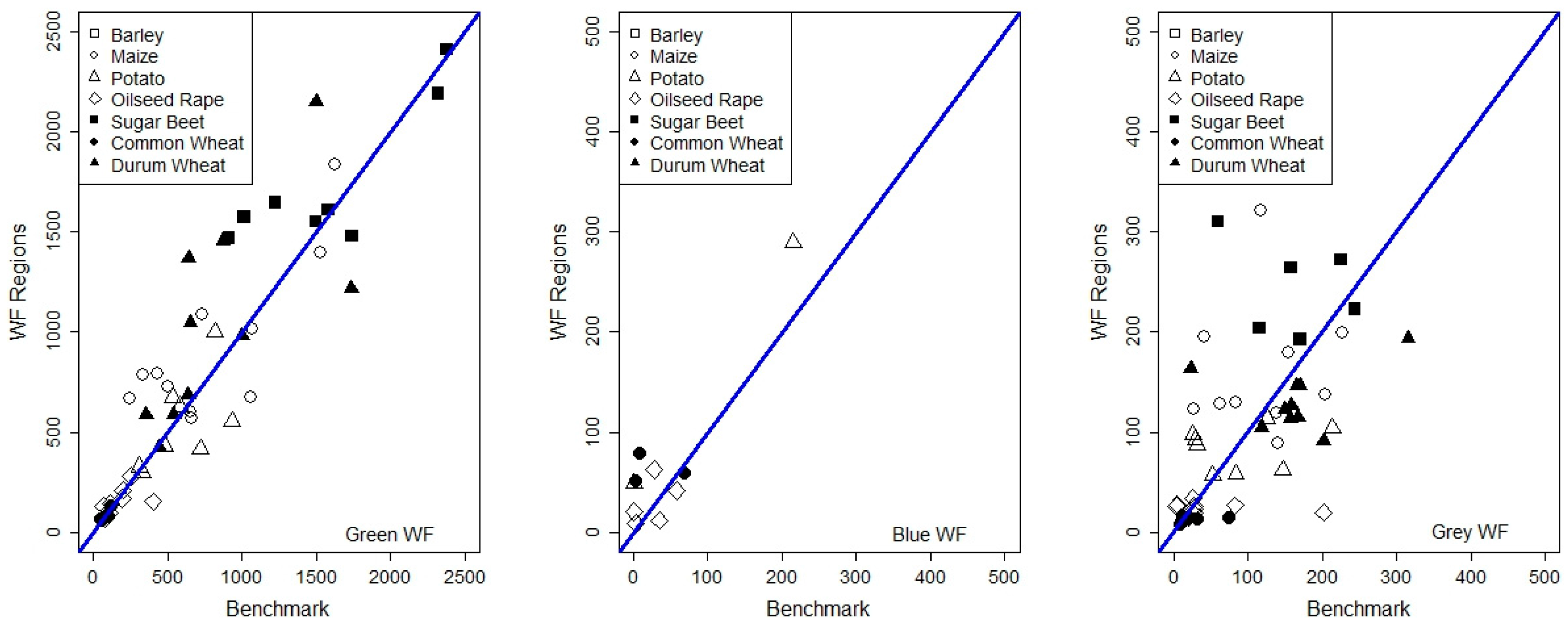
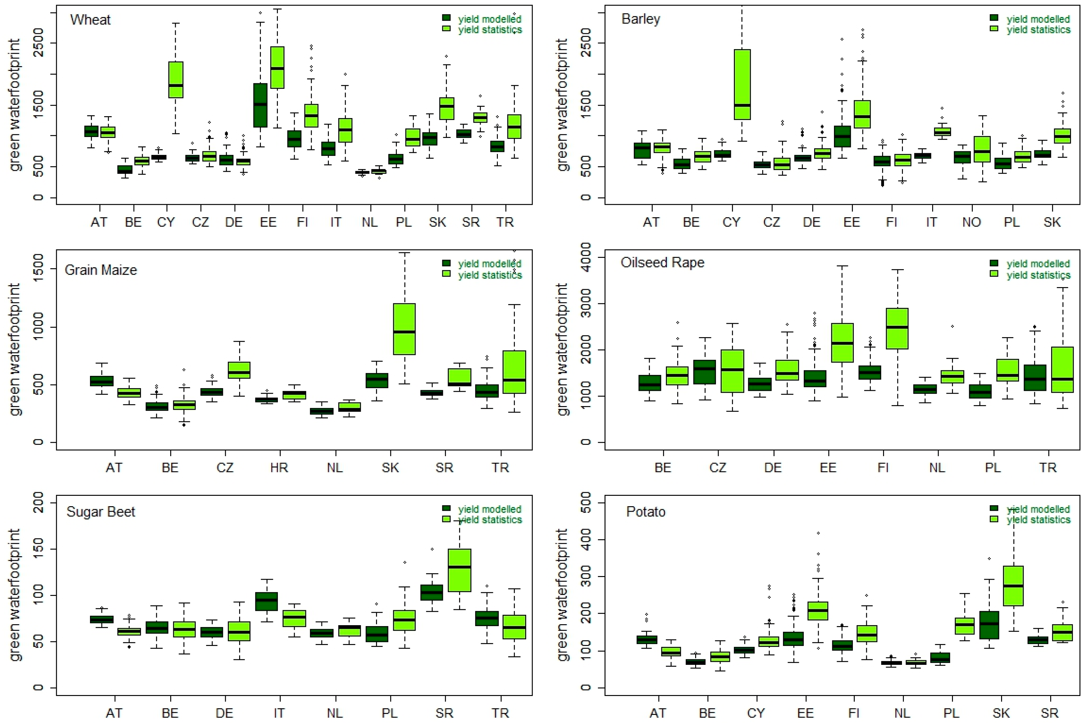
3.4. Green, Blue and Grey Water Footprint
4. Discussion
5. Conclusions
Acknowledgments
Author Contributions
Conflicts of Interest
Appendix A

| CTRY | Location | Soil Type | Texture 1 | FC (%) | WP (%) | Pore Space | References |
|---|---|---|---|---|---|---|---|
| AT | Gross Enzersdorf | Chernozem | Silt Loam | 35 | 21 | 43 | [32] |
| AT | Gross Enzersdorf | Parachernozem | Sandy Loam | 28 | 8 | 39 | |
| AT | Gross Enzersdorf | Fluvisol | Clay Loam | 35 | 22 | 42 | |
| AT | Fuchsenbigl | Calcaric Chernozem | Silt Loam | 38 | 23 | 53 | |
| BE | Koksijde | Calcaric & Gleyic Fluvisol | Marine Clay | 39 | 23 | 50 | [33,34,35] |
| BE | Gent | Albeluvisol | Sandy Loam | 22 | 10 | 47 | |
| BE | Peer | Podzol | Loamy Sand | 16 | 8 | 46 | |
| BE | Ukkel | Luvisol | Silty Loam | 34 | 12 | 49 | |
| CY | Larnaca | Chromic Vertisol | Clay | 42 | 28 | 50 | [36,37] |
| CY | Nicosia | Vertic-Chromic Luvisol | Clay Loam | 38 | 24 | 46 | |
| CY | Pafos | Eutric Fluvisol | Loam | 32 | 18 | 46 | |
| CZ | Domaninek | Dystric Cambisol | Loam | 30 | 15 | 47 | [38] |
| CZ | Lednice | Chernozem | Silt Loam | 35 | 16 | 49 | |
| CZ | Verovany | Chernozem | Silt Loam | 33 | 14 | 47 | |
| DE | Manschnow | Fluvic Gleysol | Clay loam | 39 | 15 | 46 | [39] |
| DE | Manschnow | Cambisol | Sandy Loam | 31 | 9 | 40 | [39] |
| DE | Manschnow | Podzol | Sandy Loam | 14 | 5 | 42 | [39] |
| DE | Müncheberg | Eutric Cambisol | Loamy sand | 26 | 11 | 36 | [40,41] |
| DE | Braunschweig | Luvisol | Sandy Loam | 24 | 6 | 46 | [41] |
| EE | Kuusiku | Calcic Luvisol | Silt Loam | 28 | 7 | 40 | [42] |
| EE | Väike-Maarja | Calcaric Cambisol | Sandy Loam | 28 | 8 | 45 | |
| EE | Tartu | Mollic Cambisol | Loam | 30 | 9 | 48 | |
| EE | Võru | Stagnic Luvisol | Loamy Sand | 20 | 6 | 42 | |
| EE | Tallinn | Haplic Albeluvisol | Sand | 16 | 3 | 44 | |
| EE | Kuressaare | Gleysol | Clay | 35 | 22 | 50 | |
| EE | Pärnu | Gleysol | Clay loam | 32 | 20 | 48 | |
| FI | Jokioinen | Haplic Umbrisol | Silt loam | 35 | 21 | 45 | [43] |
| FI | Mikkeli | Mollic Cambisol | Sandy Loam | 28 | 7 | 42 | |
| FI | Ylistaro | Verti-Gleyic Cambisol | Silt Loam | 35 | 15 | 48 | |
| FI | Laukaa | Eutric Regosol | Silty Clay | 46 | 25 | 55 | |
| FI | Piikiö | Vertic Cambisol | Clay Loam | 36 | 22 | 48 | |
| HR | Križevci | Gleyic Luvisol | Silt loam | 36 | 12 | 41 | [44] |
| IT | Foggia | Alluvial vertisol | Clay Loam | 42 | 24 | 55 | [45] |
| IT | Radicofani | Vertic Cambisol | Silty Clay | 42 | 27 | 51 | [46,47] |
| NL | Lelystad | Gleyic Fluvisol | Marine Clay | 36 | 16 | 45 | [48] |
| NO | Søråsjordet | Gleyic Podzoluvisol | Silt Loam | 37 | 20 | 50 | [49] |
| PL | Dąbrowice | Podzol | Loamy Sand | 23 | 17 | 40 | |
| SK | Jasl.Bohunice | Chernozem | Silty Loam | 34 | 14 | 44 | [50] |
| SK | Nitra | Luvisol | Clay Loam | 36 | 17 | 44 | |
| SK | Bratislava | Fluvisol | Sandy Loam | 32 | 12 | 44 | |
| SK | Hurbanovo | Phaeozem | Clay Loam | 35 | 18 | 44 | |
| SR | Rimski Sancevi | Chernozem | Loam | 34 | 17 | 51 | [51] |
| TR | Kirklareli | Cambisol | Sandy Clay Loam | 35 | 17 | 42 | [52] |
| TR | Tekirdağ | Fluvic Cambisol | Sandy Clay Loam | 39 | 28 | 46 | [53] |
| TR | Edirne | Cambisol | Clay Loam | 37 | 23 | 41 | [53] |
| Region * | WHB/WHD | BAR | RAP | MAZ | POT | SBT |
|---|---|---|---|---|---|---|
| P; H | P; H | P; H | P; H | P; H | P; H | |
| AT | 12/10; 30/7 | 25/3; 30/6 | 7/5; 26/9 | 16/4; 5/9 | 12/4; 18/8 | |
| BE | 15/10; !/8 | 15/10; 15/7 | 15/9; 15/7 | 1/5; 30/9 | 10/4; 30/9 | 10/4; 15/10 |
| CY | 15/11; 30/5 | 15/11; 4/5 | 15/1; 24/5 | |||
| CZ | 3/10; 30/7 | 30/3; 25/7 | 28/8; 20/7 | 30/4; 15/9 | ||
| DE-1 | 2/10; 30/7 | 20/9; 15/7 | 28/8; 24/7 | 16/5; 15/9 | ||
| DE-2 | 25/10; 30/7 | 25/9; 25/6 | 15/4; 30/9 | |||
| EE | 30/8; 10/8 | 25/4; 3/8 | 1/5; 15/9 | 5/5; 10/9 | ||
| FI-1 | 30/8; 20/8 | 15/5; 20/8 | 15/5; 10/9 | 15/5; 10/9 | ||
| FI-2 | 10/9; 15/8 | 10/5; 15/8 | 10/5; 1/9 | 15/5; 5/9 | ||
| HR | 29/4; 3/10 | |||||
| IT-1 | 15/11; 20/6 | 22/3; 18/8 | ||||
| IT-2 | 15/11; 15/7 | 15/11; 10/7 | ||||
| NL | 20/10; 30/7 | 5/9; 17/7 | 30/4; 15/10 | 25/4; 20/9 | 10/4; 15/10 | |
| NO | 25/4; 15/8 | |||||
| PL | 20/9; 14/7 | 24/4; 16/7 | 28/8; 17/8 | 15/4; 30/9 | 15/4; 20/9 | |
| SK | 7/10; 20/7 | 24/3; 10/7 | 20/4; 3/9 | 15/4; 15/9 | ||
| SR | 15/11; 10/7 | 20/4; 30/9 | 30/3; 10/7 | 30/3; 15/10 | ||
| TR | 15/11; 30/6 | 30/9; 15/6 | 9/4; 20/8 | 15/3; 20/8 |
References
- Hoekstra, A.Y.; Mekonnen, M.M. The water footprint of humanity. Proc. Natl. Acad. Sci. USA 2012, 109, 3232–3237. [Google Scholar] [CrossRef] [PubMed]
- Ciais, P.; Reichstein, M.; Viovy, N.; Granier, A.; Ogée, J.; Allard, V.; Aubinet, M.; Buchmann, N.; Bernhofer, C.; Carrara, A.; et al. Europe-wide reduction in primary productivity caused by the heat and drought in 2003. Nature 2005, 437, 529–533. [Google Scholar] [CrossRef] [PubMed]
- COPA-COGECA. COPA-COGECA. Assessment of the impact of the heat wave and drought of the summer of 2003 on agriculture and forestry. In Fact Sheets of the Committee of Agricultural Organisations in the European Union and the General Committee for Agricultural Cooperation in the European Union; COPA-COGECA: Brussels, Belgium, 2003. [Google Scholar]
- Dai, A. Increasing drought under global warming in observations and models. Nat. Clim. Chang. 2013, 3, 52–58. [Google Scholar] [CrossRef]
- Trnka, M.; Olesen, J.E.; Kersebaum, K.C.; Skjelvag, A.O.; Eitzinger, J.; Seguin, B.; Peltonen Sainio, P.; Rotter, R.; Iglesias, A.; Orlandini, S.; et al. Agroclimatic conditions in Europe under climate change. Glob. Chang. Biol. 2011, 17, 2298–2318. [Google Scholar] [CrossRef] [Green Version]
- Trnka, M.; Hlavinka, P.; Semenov, M.A. Adaptation options for wheat in Europe will be limited by increased adverse weather events under climate change. J. R. Soc. Interface 2015, 12, 20150721. [Google Scholar] [CrossRef] [PubMed]
- Damerau, K.; Patt, A.G.; van Vliet, O.P. Water saving potentials and possible trade-offs for future food and energy supply. Glob. Environ. Chang. 2016, 39, 15–25. [Google Scholar] [CrossRef]
- Allan, J.A. Virtual water: A strategic resource, global solutions to regional deficits. Ground Water 1998, 36, 545–546. [Google Scholar] [CrossRef]
- Zoumides, C.; Bruggeman, A.; Hadjikakou, M.; Zachariadis, T. Policy-relevant indicators for semi-arid nations: The water footprint of crop production and supply utilization of Cyprus. Ecol. Indic. 2014, 43, 205–214. [Google Scholar] [CrossRef]
- Ridoutt, B.G.; Pfister, S. A revised approach to water footprinting to make transparent the impacts of consumption and production on global freshwater scarcity. Glob. Environ. Chang. 2010, 20, 113–120. [Google Scholar] [CrossRef]
- International Organization for Standardization. ISO 14046: 2014: Environmental Management: Water Footprint—Principles, Requirements and Guidelines; International Organization for Standardization: Geneva, Switzerland, 2014. [Google Scholar]
- Chenoweth, J.; Hadjikakou, M.; Zoumides, C. Quantifying the human impact on water resources: A critical review of the water footprint concept. Hydrol. Earth Syst. Sci. 2014, 18, 2325–2342. [Google Scholar] [CrossRef] [Green Version]
- Mekonnen, M.M.; Hoekstra, A.Y. The green, blue and grey water footprint of crops and derived crop products. Hydrol. Earth Syst. Sci. 2011, 15, 1577–1600. [Google Scholar] [CrossRef] [Green Version]
- Chukalla, A.D.; Krol, M.S.; Hoekstra, A.Y. Green and blue water footprint reduction in irrigated agriculture: Effect of irrigation techniques, irrigation strategies and mulching. Hydrol. Earth Syst. Sci. 2015, 19, 4877–4891. [Google Scholar] [CrossRef]
- Zhuo, L.; Mekonnen, M.M.; Hoekstra, A.Y. The effect of inter-annual variability of consumption, production, trade and climate on crop-related green and blue water footprints and inter-regional virtual water trade: A study for China (1978–2008). Water Res. 2016, 94, 73–85. [Google Scholar] [CrossRef] [PubMed]
- Mekonnen, M.M.; Hoekstra, A.Y. Water footprint benchmarks for crop production: A first global assessment. Ecol. Indic. 2014, 46, 214–223. [Google Scholar] [CrossRef]
- Allen, R.G.; Pereira, L.S.; Raes, D.; Smith, M. Crop Evapotranspiration—Guidelines for Computing Crop Water Requirements; FAO Irrigation and Drainage Paper; Food and Agriculture Organization: Rome, Italy, 1998; p. D05109. [Google Scholar]
- FAO Crop-Model to Simulate Yield Response to Water. Available online: http://www.fao.org/nr/water/aquacrop.html (accessed on 23 August 2016).
- Steduto, P.; Hsiao, T.C.; Raes, D.; Fereres, E. AquaCrop—The FAO crop model to simulate yield response to water: I. Concepts and underlying principles. Agron. J. 2009, 101, 426–437. [Google Scholar] [CrossRef]
- Raes, D.; Steduto, P.; Hsiao, T.C.; Fereres, E. Aquacrop the FAO crop model to simulate yield response to water: II. Main algorithms and software description. Agron. J. 2009, 101, 438–447. [Google Scholar] [CrossRef]
- Kersebaum, K.C.; Kroes, J.; Gobin, A.; Takác, J.; Hlavinka, P.; Trnka, M.; Ventrella, D.; Giglio, L.; Ferrise, R.; Moriondo, M.; et al. Assessing the uncertainty of model based water footprint estimation using an ensemble of crop growth models on winter wheat. Water 2016, 8, 571. [Google Scholar] [CrossRef]
- Rockström, J.; Falkenmark, M.; Karlberg, L.; Hoff, H.; Rost, S.; Gerten, D. Future water availability for global food production: The potential of green water for increasing resilience to global change. Water Res. 2009, 45, W00A12. [Google Scholar] [CrossRef]
- Eurostat. Gross Nutrient Balance. Available online: http://ec.europa.eu/eurostat/cache/metadata/EN/aei_pr_gnb_esms.htm (accessed on 23 August 2016).
- World Bank, Fertilizer Consumption Rates per Hectare of Arable Land. Available online: http://databank.worldbank.org/data/reports.aspx?source=2&series=AG.CON.FERT.ZS&country (accessed on 23 August 2016).
- Eurostat. Handbook for Annual Crop Statistics. European Commission-Eurostat, Directorate E Sectoral and Regional Statistics, Unit E1 Agriculture and Fisheries. Available online: http://ec.europa.eu/eurostat/cache/metadata/Annexes/apro_acs_esms_an1.pdf (accessed on 23 August 2016).
- R Core Group. The R Project for Statistical Computing. Available online: https://www.r-project.org/ (accessed on 20 November 2016).
- Zambrano-Bigiarini, M. hydroGOF: Goodness-of-Fit Functions for Comparison of Simulated and Observed Hydrological Time Series. 2011. R Package Version 0.3-2. Available online: http://CRAN.R-project.org/package=hydroGOF (accessed on 23 August 2016).
- Evett, S.R.; Tolk, J.A. Introduction: Can Water Use Efficiency Be Modeled Well Enough to Impact Crop Management? Agron. J. 2009, 101, 423–425. [Google Scholar] [CrossRef]
- Mekonnen, M.M.; Hoekstra, A.Y. The Green, Blue and Grey Water Footprint of Crops and Derived Crop Products. Value of Water Research Report Series No. 47. UNESCO-IHE: Delft, The Netherlands, 2010. Available online: http://www.waterfootprint.org/Reports/Report47-WaterFootprintCrops-Vol1.pdf (accessed on 23 August 2016).
- Velthof, G.L.; Lesschen, J.P.; Webb, J.; Pietrzak, S.; Miatkowski, Z.; Pinto, M.; Kros, J.; Oenema, O. The impact of the Nitrates Directive on nitrogen emissions from agriculture in the EU-27 during 2000–2008. Sci. Total Environ. 2014, 468, 1225–1233. [Google Scholar] [CrossRef] [PubMed]
- Mekonnen, M.M.; Hoekstra, A.Y. Global gray water footprint and water pollution levels related to anthropogenic nitrogen loads to fresh water. Environ. Sci. Technol. 2015, 49, 12860–12868. [Google Scholar] [CrossRef] [PubMed]
- Eitzinger, J.; Trnka, M.; Semerádová, D.; Thaler, S.; Svobodová, E.; Hlavinka, P.; Siska, B.; Takáč, J.; Malatinská, L.; Nováková, M.; et al. Regional climate change impacts on agricultural crop production in Central and Eastern Europe–hotspots, regional differences and common trends. J. Agric. Sci. 2013, 151, 787–812. [Google Scholar] [CrossRef]
- Gobin, A. Impact of heat and drought stress on arable crop production in Belgium. Natl. Hazards Earth Syst. Sci. 2012, 12, 1911–1922. [Google Scholar] [CrossRef]
- Gobin, A. Modelling climate impacts on arable yields in Belgium. Clim. Res. 2010, 44, 55–68. [Google Scholar] [CrossRef]
- Gobin, A. The water footprint of Belgian arable crops. Ital. J. Agric. Meteorol. 2015, 4, 91–97. [Google Scholar]
- Zoumides, C.; Bruggeman, A.; Zachariadis, T.; Pashiardis, S. Quantifying the poorly known role of groundwater in agriculture: The case of Cyprus. Water Resour. Manag. 2013, 27, 2501–2514. [Google Scholar] [CrossRef]
- Camera, C.; Zomeni, Z.; Noller, J.; Zissimos, A.; Christoforou, I.; Bruggeman, A. A high resolution map of soil types and physical properties for Cyprus: A digital soil mapping optimization. Geoderma 2017, 285, 35–49. [Google Scholar] [CrossRef]
- Hlavinka, P.; Trnka, M.; Kersebaum, K.; Cermak, P.; Pohankova, E.; Ors_ag, M.; Pokorný, E.; Fischer, M.; Brtnický, M.; Zalud, Z. Modelling of yields and soil nitrogen dynamics for crop rotations by HERMES under different climate and soil conditions in the Czech Republic. J. Agric. Sci. 2014, 152, 188–204. [Google Scholar] [CrossRef]
- Kersebaum, K.C.; Nendel, C. Site-specific impacts of climate change on wheat production across regions of Germany using different CO2 response functions. Eur. J. Agron. 2014, 52, 22–32. [Google Scholar] [CrossRef]
- Mirschel, W.; Barkusky, D.; Hufnagel, J.; Kersebaum, K.C.; Nendel, C.; Laacke, L.; Luzi, K.; Rosner, G. Coherent multi-variable field data set of an intensive cropping system for agro-ecosystem modelling from Müncheberg, Germany. Open Data J. Agric. Res. 2016, 2, 1–10. [Google Scholar] [CrossRef]
- Kollas, C.; Kersebaum, K.C.; Nendel, C.; Manevski, K.; Müller, C.; Palosuo, T.; Armas-Herrera, C.M.; Beaudoin, N.; Bindi, M.; Charfeddine, M.; et al. Crop rotation modelling–a European model intercomparison. Eur. J. Agron. 2015, 70, 98–111. [Google Scholar] [CrossRef]
- Kadaja, J.; Saue, T. Effects of different irrigation and drainage regimes on yield and water productivity of two potato varieties under Estonian temperate climate. Agric. Water Manag. 2016, 165, 61–71. [Google Scholar] [CrossRef]
- Peltonen-Sainio, P.; Jauhiainen, L.; Hakala, K. Crop responses to temperature and precipitation according to long-term multi-location trials at high-latitude conditions. J. Agric. Sci. 2011, 149, 49–62. [Google Scholar] [CrossRef]
- Vučetić, V. Modelling of maize production in Croatia: Present and future climate. J. Agric. Sci. 2011, 149, 145–157. [Google Scholar] [CrossRef] [PubMed]
- Ventrella, D.; Stellacci, A.M.; Castrignanò, A.; Charfeddine, M.; Castellini, M. Effects of crop residue management on winter durum wheat productivity in a long term experiment in Southern Italy. Eur. J. Agron. 2016, 77, 188–198. [Google Scholar] [CrossRef]
- Dalla Marta, A.; Orlando, F.; Mancinii, M.; Guasconi, F.; Motha, R.; Qu, J.; Orlandini, S. A simplified index for an early estimation of durum wheat yield in Tuscany (Central Italy). Field Crops Res. 2015, 170, 1–6. [Google Scholar] [CrossRef]
- Guasconi, F.; Dalla Marta, A.; Grifono, D.; Mancini, M.; Orlando, F.; Orlandini, S. Influence of climate on durum wheat production and use of remote sensing and weather data to predict quality and quantity of harvests. Ital. J. Agrometeorol. 2011, 3, 21–28. [Google Scholar]
- Van Bakel, P.J.T.; Massop, H.T.L.; Kroes, J.G.; Hoogewoud, J.; Pastoors, R.; Kroon, T. Actualisatie Hydrologie voor STONE 2.3. In Aanpassing Randvoorwaarden en Parameters, Koppeling Tussen NAGROM en SWAP, en Plausibiliteitstoets; WOt-Rapport 57; Wettelijke Onderzoekstaken Natuur & Milieu (MNP), Alterra: Wageningen, The Netherlands, 2008. [Google Scholar]
- Deelstra, J.; Kværnø, S.H.; Skjevdal, R.; Vandsemb, S.; Eggestad, H.O.; Ludvigsen, G.H. A General Description of Skuterud Catchment; Jordforsk (Now NIBIO) Report No. 61/05; Bioforsk: Ås, Norway, 2005. [Google Scholar]
- Takáč, J.; Skalský, R.; Morávek, A.; Klikušovská, Z.; Bezák, P.; Bárdyová, M. Spatial Patterns of Agricultural Drought Events in Danube Lowland in the 1961–2013 Period. In Proceedings of the International Scientific Conference towards Climatic Services, Nitra, Slovakia, 15–18 September 2015.
- Stričević, R.; Cosić, M.; Djurović, N.; Pejić, B.; Maksimović, L. Assessment of the FAO “Aquacrop” model in the simulation of rainfed and supplementally-irrigated maize, sugar beet and sunflower. Agric. Water Manag. 2011, 98, 1615–1621. [Google Scholar]
- Şaylan, L.; Çaldağ, B.; Bakanoğulları, F. Investigation of Potential Effects of Climate Change on Crop Growth by Crop Growth Simulation Models; TUBITAK Project No.: 1080567; TUBITAK: Istanbul, Turkey, 2012; p. 258. (In Turkish) [Google Scholar]
- Çakir, R. Istranca (Yıldız) Dağı Güneyinde Yer Alan Vertisol Ordosu Topraklarının Toprak Taksonomisine Göre Belirlenmesi, Toprak ve Su Mühendisliği Yönünden İrdelenmesi. Ph.D. Thesis, Trakya Üniversitesi, Edirne, Turkey, 1997. [Google Scholar]


| Country Region | Meteo Stations 1 | Major Crops 2 | |
|---|---|---|---|
| AT | Marchfeld | Gross Enzersdorf, Fuchsenbigl | WHB, BAR, MAZ, SBT |
| BE | Flanders | Koksijde, Gent, Ukkel, Peer | WHB, BAR, MAZ, SBT, POT |
| CY | Country | Nicossia, Pafos, Larnaca | WHD, POT, BAR, MAZ |
| CZ | Eastern Czech | Domaninek, Lednice, Verovany | WHB, BAR, MAZ, RAP |
| DE-1 | Märk. Oderland | Muncheberg, Manschnow | WHB, BAR, SBT, RAP, POT, MAZ |
| DE-2 | North-East Lower Saxony | Braunschweig | WHB, BAR, SBT |
| EE | Country | Kuusiku, Tartu, Tallinn, Võru, Pärnu, Väike-Maarja, Kuressaare | WHB, BAR, POT, RAP |
| FI-1 | Häme | Jokioinen | BAR, WHB, BAR, POT, RAP |
| FI-2 | South Finland | Mikkeli, Ylistaro, Laukaa, Piikio | BAR, WHB, BAR, POT, RAP |
| HR | Koprivnica-Križevci | Križevci | MAZ |
| IT-1 | Foggia | Foggia | WHD, SBT |
| IT-2 | Val d’Orcia | Radicofani | WHB, WHD, BAR |
| NO | South Eastern Norway | Søråsjordet | BAR |
| NL | Flevoland | Lelystad | WHB, POT, SBT, MAZ |
| PL | Mazovia | Dąbrowice | WHB, BAR, POT, SBT, RAP |
| SK | Danube Lowland | Bratislava-letisko, Hurbanovo, Nitra, Jaslovske Bohunice | WHB, BAR, MAZ |
| SR | Vojvodina | Rimski Sancevi | WHD, MAZ, SBT, POT |
| TR | Thrace | Edirne, Kırklareli, Tekirdağ | WHD, WHB, BAR, MAZ |
| Crop | ystat·m | ystat·s | ystat·cv | ymod·m | ymod·s | ymod·cv | HI |
|---|---|---|---|---|---|---|---|
| BAR | 4.44 | 1.86 | 41.88 | 5.26 | 1.77 | 33.54 | 41 |
| MAZ | 7.76 | 2.92 | 37.67 | 9.28 | 2.27 | 24.50 | 41 |
| POT | 28.07 | 12.60 | 44.88 | 33.58 | 13.89 | 41.35 | 72 |
| RAP | 2.48 | 1.10 | 44.50 | 3.04 | 0.92 | 30.26 | 23 |
| SBT | 52.43 | 11.55 | 22.02 | 54.24 | 12.74 | 23.48 | 64 |
| WHB | 4.94 | 2.04 | 41.27 | 6.13 | 1.96 | 31.91 | 41 |
| WHD | 3.05 | 0.85 | 27.99 | 4.96 | 0.86 | 17.43 | 37 |
| Crop | WFg·m | WFg·s | WFg·cv | ET·m | ET·s | ET·cv |
|---|---|---|---|---|---|---|
| RAP | 1857 | 661 | 36 | 405 | 103 | 25 |
| WHB | 1108 | 580 | 52 | 459 | 87 | 19 |
| WHD | 1414 | 720 | 51 | 375 | 62 | 17 |
| BAR | 901 | 458 | 51 | 337 | 82 | 24 |
| MAZ | 590 | 304 | 52 | 373 | 73 | 20 |
| POT | 157 | 75 | 48 | 332 | 64 | 19 |
| SBT | 67 | 19 | 29 | 351 | 86 | 25 |
© 2017 by the authors. Licensee MDPI, Basel, Switzerland. This article is an open access article distributed under the terms and conditions of the Creative Commons Attribution (CC BY) license ( http://creativecommons.org/licenses/by/4.0/).
Share and Cite
Gobin, A.; Kersebaum, K.C.; Eitzinger, J.; Trnka, M.; Hlavinka, P.; Takáč, J.; Kroes, J.; Ventrella, D.; Marta, A.D.; Deelstra, J.; et al. Variability in the Water Footprint of Arable Crop Production across European Regions. Water 2017, 9, 93. https://doi.org/10.3390/w9020093
Gobin A, Kersebaum KC, Eitzinger J, Trnka M, Hlavinka P, Takáč J, Kroes J, Ventrella D, Marta AD, Deelstra J, et al. Variability in the Water Footprint of Arable Crop Production across European Regions. Water. 2017; 9(2):93. https://doi.org/10.3390/w9020093
Chicago/Turabian StyleGobin, Anne, Kurt Christian Kersebaum, Josef Eitzinger, Miroslav Trnka, Petr Hlavinka, Jozef Takáč, Joop Kroes, Domenico Ventrella, Anna Dalla Marta, Johannes Deelstra, and et al. 2017. "Variability in the Water Footprint of Arable Crop Production across European Regions" Water 9, no. 2: 93. https://doi.org/10.3390/w9020093