Depth-Averaged Non-Hydrostatic Hydrodynamic Model Using a New Multithreading Parallel Computing Method

Abstract

Compared to the hydrostatic hydrodynamic model, the non-hydrostatic hydrodynamic model can accurately simulate flows that feature vertical accelerations. The model’s low computational efficiency severely restricts its wider application. This paper proposes a non-hydrostatic hydrodynamic model based on a multithreading parallel computing method. The horizontal momentum equation is obtained by integrating the Navier–Stokes equations from the bottom to the free surface. The vertical momentum equation is approximated by the Keller-box scheme. A two-step method is used to solve the model equations. A parallel strategy based on block decomposition computation is utilized. The original computational domain is subdivided into two subdomains that are physically connected via a virtual boundary technique. Two sub-threads are created and tasked with the computation of the two subdomains. The producer–consumer model and the thread lock technique are used to achieve synchronous communication between sub-threads. The validity of the model was verified by solitary wave propagation experiments over a flat bottom and slope, followed by two sinusoidal wave propagation experiments over submerged breakwater. The parallel computing method proposed here was found to effectively enhance computational efficiency and save 20%–40% computation time compared to serial computing. The parallel acceleration rate and acceleration efficiency are approximately 1.45% and 72%, respectively. The parallel computing method makes a contribution to the popularization of non-hydrostatic models.

1. Introduction

The propagation of sea waves from the abyssal zone to the shoal involves a series of complex physical processes such as wave refraction, wave diffraction, and shoaling. Many researchers have explored these physical mechanisms by reproducing wave propagation and transformation experimentally and have analyzed the prototype experiments using mathematical models [1,2,3], including the Boussinesq-type equation [4,5], a potential flow model based on the Laplace equation, and a non-hydrostatic hydrodynamic model.

Based on the hydrostatic assumptions, the hydrodynamic models can be split into hydrostatic and non-hydrostatic categories. Non-hydrostatic models consider the effect of dynamic pressure on the flow field, and are thus appropriate for situations with significant vertical acceleration; hydrostatic models are not. Thus non-hydrostatic models can more accurately reveal the discipline of flow movement, and are particularly well suited to complex numerical simulations of wave propagation. Non-hydrostatic models have substantial research value, as they contribute to a better understanding of the wave conditions in inshore areas and provide technical support for inshore breakwater and coastal works designs. Current non-hydrostatic models are plagued by two major issues: (1) managing the dynamic pressure variable (non-hydrostatic) and (2) relatively unfavorable computational efficiency.

Managing the dynamic pressure variable is the key to successful non-hydrostatic modeling. In most non-hydrostatic models, it is assumed that the pressure of the surface grid conforms to the hydrostatic distribution and the dynamic pressure variables are placed at the center of the surface grid [6,7]. Thus these models do not completely deviate from the hydrostatic assumption. To enable the model to strictly meet the zero dynamic pressure boundary conditions at the free water surface, Stelling and Zijlema proposed that the dynamic pressure variable should be placed at the center of the upper and lower interface of the grid [8]. This allows zero dynamic pressure boundary conditions to be directly satisfied when the dynamic pressure at the water surface is assumed to be zero. They built a 3D model based on this dynamic pressure layout; the model can accurately simulate the frequency dispersion characteristics and the nonlinear effect of short wave with only two layers in the vertical direction. In another study, Bai and Cheung uniformly divided the water into two layers and parameterized the dynamic pressure at the interface between the layers [9,10]. The θ method was used to discretize the momentum equation based on the structured grid. This model can accurately simulate the complex solitary wave propagation over a fringing reef. Another so called non-hydrostatic top-layer treatment method was proposed by Yuan and Wu [11], in which the dynamic pressure variables are still placed at the center of the surface grid and the vertical momentum equation is integrated from the center of the top layer to the free surface, so the top-layer pressure can be explicitly expressed by the hydrostatic pressure component and vertical acceleration. This method also satisfies the zero dynamic pressure condition. Later, they further extended the non-hydrostatic top-layer treatment method to the Cartesian co-ordinate [12]. Namin et al. used a hydrostatic representation to define the pressure term in the top layer so that it can be evaluated in terms of the neighboring horizontal velocity components alone [13]. With this treatment, they developed a 2D vertical numerical model to simulate a range of unsteady flow problems involving relatively strong vertical accelerations.

Non-hydrostatic models are now more commonly utilized for 3D simulation [6,14,15]. The 3D model can truly reflect changes in the flow field of the natural fluid in 3D directions. The number of computational grids necessary for such large-scale fluid domains such as seas is often very large, therefore, making it effectually impossible to solve the 3D model equations. Over the past decade, many efforts have been devoted to develop 3D non-hydrostatic models with a few vertical layers. Yuan and Wu developed an implicit method for solving the 3D fully non-hydrostatic model [12]. The 3D model has been proven capable of accurately simulating a range of free-surface flow problems using a very small number of vertical layers. Later, they examined the accuracy and efficiency of their fully non-hydrostatic model by simulating a range of surface-wave propagation problems [16]. Bai and Cheung developed a new multi-layer non-hydrostatic model and examined its linear and nonlinear wave properties in relation to the Boussinesq approach [17]. Young et al. developed a higher-order non-hydrostatic σ model with only two vertical layers, and verified its accuracy via laboratory data [18]. Furthermore, researchers have also developed a number of 2D horizontal models and vertical models. Due to the reduction of one spatial dimension, the amount of computational work of the 2D non-hydrostatic models decreases significantly and the computational efficiency increases significantly. Zhou and Stansby established the first vertical 2D non-hydrostatic model [7]. Stelling and Busnelli used a vertical 2D non-hydrostatic model to successfully simulate the hydraulic jump [19], which cannot be simulated by a hydrostatic model. Their results also demonstrated that the non-hydrostatic model has higher accuracy and broader application prospects than the hydrostatic model. Ling Kang, one author of this paper, derived depth-averaged 2D horizontal non-hydrostatic model equations and verified the validity of the model using a series of benchmark tests [20]. These 2D models have higher computational efficiency than the 3D models, but complex and time-consuming iterative methods (e.g., the gradient method) are necessary to solve the large-scale Pressure Poisson Equations (PPEs), thus, the low computational efficiency problem inherent to the non-hydrostatic model has not been effectively resolved.

The above shows that computational efficiency is one of the critical factors for determining whether the non-hydrostatic model can substitute the hydrostatic models as the next-generation tool for simulating the flow in large-scale environments. The solution to this problem is transferring the numerical computation from a single-core environment to a multi-core environment. To this end, parallel computation has become a popular approach when researching non-hydrostatic models. Non-hydrostatic model codes have typical serial characteristics. The parallelization of the serial codes is very difficult, so there have been relatively few attempts to do so. Jacek et al. developed a parallelization method for an unstructured-grid 3D non-hydrostatic model based on a new parallel streamline backtracking algorithm. The parallel performance was investigated on shared-memory, massive parallel computing servers; the results showed that their method does substantially enhance computational efficiency [21]. Hérault et al. simulated paddle-generated waves in a basin and a dam-break wave based on the GPU parallel technique and the SPH (Smoothed Particle Hydrodynamics) method. Their simulation speed was one to two orders of magnitude faster than the equivalent CPU code [22]. Bleichrodt et al. presented a 2D barotropic vorticity model on a GPU using a CUDA implementation. The speed-up for this model is impressive: up to a factor of 50 for the highest resolutions [23]. These parallel computational methods do significantly improve the computational efficiency of the non-hydrostatic model and yield a desirable speed-up ratio, but they are largely dependent on high-performance cluster groups or GPU, which come with a high technical threshold. Many researchers who are familiar with non-hydrostatic models are not experts in fluid computing. Reproducing or modifying the complicated frontier parallelization methods requires very demanding technical conditions and consumes a great deal of resources (money, time, talent cultivation). In addition, current parallel programs—whether they function via a shared memory mode (such as OpenMP) or the message passing mode (such as MPI)—are typically developed in the Linux System or Unix System. There have been few researchers to attempt to establish these models in the Windows environment. Nesterov proposed a simple parallelization technique with MPI in Windows for 2D ocean circulation models [24]. Windows users outnumber the users of other operating systems, but most of the open-source parallelized CFD codes do not run on Windows. It is not easy for Windows users with only basic coding knowledge to reproduce or modify the extant parallelization methods on a computer with a minimum of memory and hardware. Thus, to further popularize non-hydrostatic models, it is imperative to design a simple, efficient parallel computing method in the Windows system for researchers who are experts in CFD models with basic coding knowledge.

From the above, this paper proposes a non-hydrostatic hydrodynamic model based on a multithreading parallel computing method suited to the Windows system. A parallel strategy based on block decomposition computation is utilized. Based on the Windows multithreading mechanism, two sub-threads are created and tasked computation of the two subdomains. The producer–consumer model and the thread lock technique are used to achieve synchronous communication between sub-threads. The validity of the model was verified by solitary wave experiments and sinusoidal wave experiments. The computational efficiency is discussed.

2. Mathematical Model

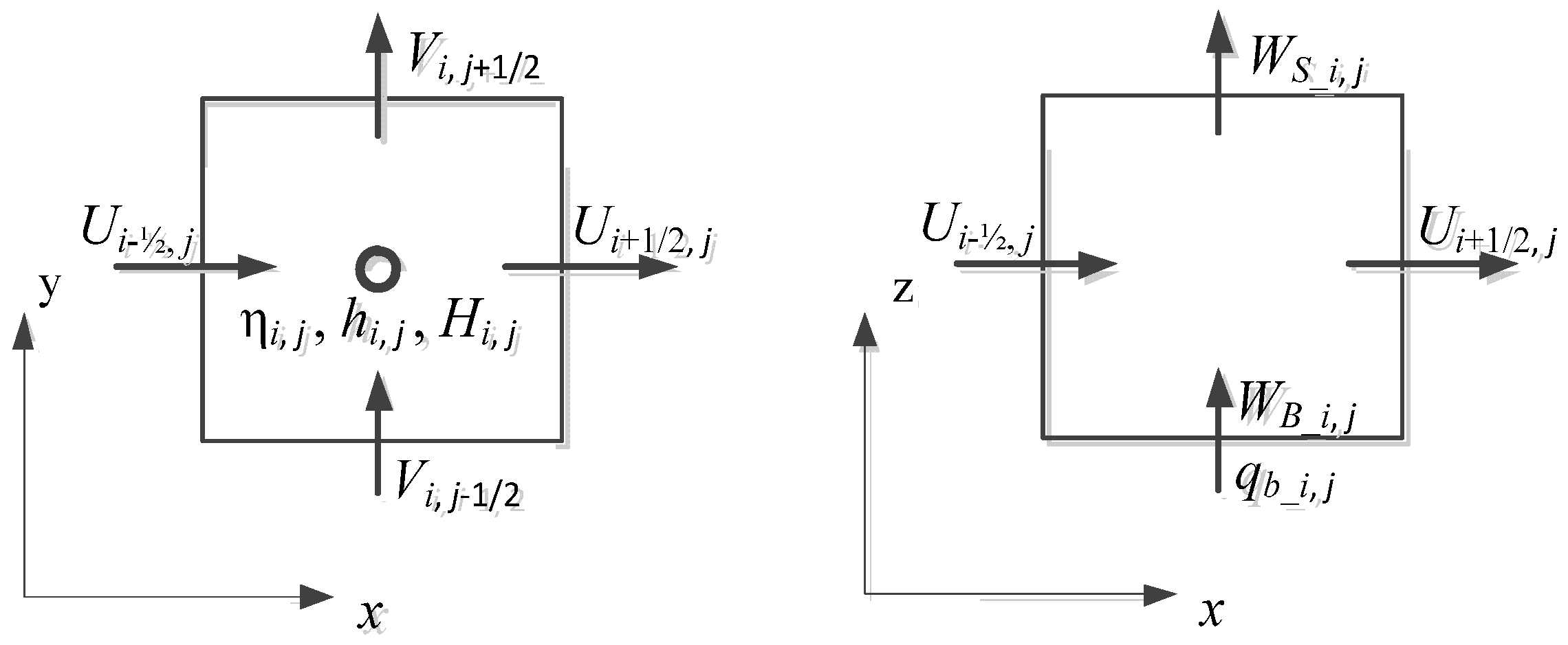
2.1. Governing Equations

To improve the hydrostatic hydrodynamic model, the pressure term in the 3D Navier–Stokes (N–S) equations is separated into hydrostatic and non-hydrostatic components. The horizontal momentum equations and the continuity equation are integrated from bottom to free surface. The vertical momentum equation only retains the dynamic pressure gradient term. Coupling with the kinematic boundary conditions at the water bottom and free surface, the author of this paper has proposed a plane 2D, depth-integrated non-hydrostatic hydrodynamic model: Equations (1)–(5). Details can be seen in the literature [20]. This depth-integrated model is essentially applicable in coastal regions up to the shore [25]. According to Stelling and Zijlema [8], this non-hydrostatic model using one layer approximates at most the lowest order effect of linear wave dispersion, namely, it is valid when the wave is weakly dispersive (μ = kH < 1, where k and H are the wave number and still water depth, respectively). Highly dispersive cases are not considered in this paper.

$$\frac{\partial U}{\partial x}+\frac{\partial V}{\partial y}+\frac{\partial w}{\partial z}=0$$

(1)

$$\frac{\partial \mathsf{\eta }}{\partial t}+\frac{\partial (UH)}{\partial x}+\frac{\partial (VH)}{\partial y}=0$$

(2)

$$\frac{\partial U}{\partial t}+U\frac{\partial U}{\partial x}+V\frac{\partial U}{\partial y}=-g\frac{\partial \mathsf{\eta }}{\partial x}-\frac{1}{2\mathsf{\rho }}\frac{\partial q_b}{\partial x}-\frac{q_b}{2H\mathsf{\rho }}\frac{\partial (\mathsf{\eta }-h)}{\partial x}$$

(3)

$$\frac{\partial V}{\partial t}+U\frac{\partial V}{\partial x}+V\frac{\partial V}{\partial y}=-g\frac{\partial \mathsf{\eta }}{\partial y}-\frac{1}{2\mathsf{\rho }}\frac{\partial q_b}{\partial y}-\frac{q_b}{2H\mathsf{\rho }}\frac{\partial (\mathsf{\eta }-h)}{\partial y}$$

(4)

$$\frac{\partial w}{\partial t}=-\frac{1}{\rho }\frac{\partial q}{\partial z}$$

(5)

Equation (1) is the continuity equation; Equation (2) is the free surface equation; Equations (3) and (4) are the horizontal momentum equations (the Coriolis, the wind shear, and bottom friction forces are ignored); Equation (5) is the vertical momentum equation (the convective and viscosity terms are ignored). t is time (s); U and V (m/s) are the depth-averaged velocity in the x and y directions, respectively; w is the velocity in the z direction (m/s); $\mathsf{\rho }$ is water density (kg/m³); q is the dynamic (non-hydrostatic) pressure; H is the total water depth (m), H = h + η; h is the still water depth (m); η is the surface elevation above the still-water level (m).

2.2. Initial Condition and Boundary Condition

The initial condition of velocity and water level are set to zero and the still-water level, respectively; “No slip condition” is applied to the solid wall boundary condition; Velocity U at the inflow are specified based on the analytical solutions or experimental data. The analytical solution of solitary wave and sinusoidal wave can be found in the literature [26]; Velocity U at the outflow are specified using Sommerfeld’s radiation condition considering that it does not produce a reflection wave when flow is passing through the outflow [27]:

$$\frac{\partial f}{\partial t}+\sqrt{gH}\frac{\partial f}{\partial x}=0,$$

(6)

where f = U, V, η.

3. Numerical Solution

A structured C-grid scheme is used for discretization of the computational domain. The governing equations are solved by the finite difference method (FDM). Figure 1 shows the layout of variables. i and j denote the cell grid center in the x and y direction; U and V are defined at the center of the grid faces (i ± 1/2, j) and (i, j ± 1/2); η, h, and H are located at the center of the grid; The dynamic pressure q is located at the center of the top and bottom surfaces; the dynamic pressure at the bottom q_b is at the center of the bottom surface; the dynamic pressure at the free surface is set to be zero in order to satisfy the zero dynamic pressure condition; W_S and W_B, which are the vertical velocity at the free surface and bottom, are located at the center of the top and bottom surfaces, respectively.

All the terms except the dynamic pressure gradient term in Equations (3) and (4) are solved explicitly by a central difference scheme. The dynamic pressure gradient term is solved by the Crank–Nicolson scheme. Superscripts n and (n + 1) denote the time levels n and (n + 1), respectively; Δt denotes the time step; and Δx and Δy denote the length and width of the grid cell, respectively. The discrete form of Equations (3) and (4) can be written as:

$$\begin{array}{ll}{U}_{i+1/2,j}^{n+1}=& U_{i+1/2,j}^n-\frac{\Delta t}{2\Delta x}{U}_{i+1/2,j}^n(U_{i+3/2,j}^n-U_{i-1/2,j}^n)-\frac{\Delta t}{2\Delta y}{V}_{i+1/2,j}^{n*}(U_{i+1/2,j+1}^n-U_{i+1/2,j-1}^n)\\ & -g\frac{\Delta t}{\Delta x}({\mathsf{\eta }}_{i+1,j}^n-{\mathsf{\eta }}_{i,j}^n)-\frac{\Delta t}{2\mathsf{\rho }\Delta x}\frac{(q_{b\_i+1,j}^n+q_{b\_i,j}^n)({\mathsf{\eta }}_{i+1,j}^n-{\mathsf{\eta }}_{i,j}^n-h_{i+1,j}+h_{i,j})}{H_{i+1,j}^n+H_{i,j}^n}\\ & -\frac{1}{2}\frac{\Delta t}{2\mathsf{\rho }\Delta x}(q_{b\_i+1,j}^n-q_{b\_i,j}^n)-\frac{1}{2}\frac{\Delta t}{2\mathsf{\rho }\Delta x}(q_{b\_i+1,j}^{n+1}-q_{b\_i,j}^{n+1})\end{array}$$

(7)

$$\begin{array}{ll}{V}_{i,j+1/2}^{n+1}=& V_{i,j+1/2}^n-\frac{\Delta t}{2\Delta x}{U}_{i,j+1/2}^{n*}(V_{i+1,j+1/2}^n-V_{i-1,j+1/2}^n)-\frac{\Delta t}{2\Delta y}{V}_{i,j+1/2}^n(V_{i,j+3/2}^n-V_{i,j-1/2}^n)\\ & -g\frac{\Delta t}{\Delta y}({\mathsf{\eta }}_{i,j+1}^n-{\mathsf{\eta }}_{i,j}^n)-\frac{\Delta t}{2\mathsf{\rho }\Delta y}\frac{(q_{b\_i,j+1}^n+q_{b\_i,j}^n)({\mathsf{\eta }}_{i,j+1}^n-{\mathsf{\eta }}_{i,j}^n-h_{i,j+1}+h_{i,j})}{H_{i,j}^n+H_{i,j+1}^n}\\ & -\frac{1}{2}\frac{\Delta t}{2\mathsf{\rho }\Delta y}(q_{b\_i,j+1}^n-q_{b\_i,j}^n)-\frac{1}{2}\frac{\Delta t}{2\mathsf{\rho }\Delta y}(q_{b\_i,j+1}^{n+1}-q_{b\_i,j}^{n+1})\end{array},$$

(8)

where

$$U_{i,j+1/2}^{n*}=\frac{1}{4}(U_{i-1/2,j}^n+U_{i+1/2,j}^n+U_{i-1/2,j+1}^n+U_{i+1/2,j+1}^n)$$

(9)

$$V_{i+1/2,j}^{n*}=\frac{1}{4}(V_{i,j-1/2}^n+V_{i,j+1/2}^n+V_{i+1,j-1/2}^n+V_{i+1,j+1/2}^n).$$

(10)

A two-step method is used for solving Equations (7) and (8):

1. The first step

In the first step, taking Equation (7) as an example, Equation (7) retains the convective term, the water level gradient term, the combination term of dynamic pressure and water level and the dynamic pressure gredient term at the current time (superscript n), resulting in Equation (11). The intermediate value of the velocity (denoted as U^n+1/2) can be calculated by solving Equation (11).

$$\begin{array}{ll}{U}_{i+1/2,j}^{n+1/2}=& U_{i+1/2,j}^n-\frac{\Delta t}{2\Delta x}{U}_{i+1/2,j}^n(U_{i+3/2,j}^n-U_{i-1/2,j}^n)-\frac{\Delta t}{2\Delta y}{V}_{i+1/2,j}^{n*}(U_{i+1/2,j+1}^n-U_{i+1/2,j-1}^n)\\ & -g\frac{\Delta t}{\Delta x}({\mathsf{\eta }}_{i+1,j}^n-{\mathsf{\eta }}_{i,j}^n)-\frac{\Delta t}{2\mathsf{\rho }\Delta x}\frac{(q_{b\_i+1,j}^n+q_{b\_i,j}^n)({\mathsf{\eta }}_{i+1,j}^n-{\mathsf{\eta }}_{i,j}^n-h_{i+1,j}+h_{i,j})}{H_{i+1,j}^n+H_{i,j}^n}\\ & -\frac{1}{2}\frac{\Delta t}{2\mathsf{\rho }\Delta x}(q_{b\_i+1,j}^n-q_{b\_i,j}^n)\end{array}$$

(11)

2. The second step

Based on the calculated U^n+1/2 and V^n+1/2 in the first step, Equations (7) and (8) only retain the dynamic pressure gredient term at time level n+1, resulting in Equations (12) and (13).

$$U_{i+1/2,j}^{n+1}=U_{i+1/2,j}^{n+1/2}-\frac{1}{2}\frac{\Delta t}{2\mathsf{\rho }\Delta x}(q_{b\_i+1,j}^{n+1}-q_{b\_i,j}^{n+1})$$

(12)

$$V_{i,j+1/2}^{n+1}=V_{i,j+1/2}^{n+1/2}-\frac{1}{2}\frac{\Delta t}{2\mathsf{\rho }\Delta y}(q_{b\_i,j+1}^{n+1}-q_{b\_i,j}^{n+1})$$

(13)

The Keller-box scheme is used to discretize the vertical momentum equation Equation (5) [28]. This scheme has three steps. First, by the forward differencing scheme at the centre of the bottom face, the dynamic pressure gradient term can be approximated as:

$$\frac{W_{B\_i,j}^{n+1}-W_{B\_i,j}^n}{\Delta t}=-\frac{1}{\mathsf{\rho }}\frac{0-q_{b\_i,j}^{n+1}}{H_{i,j}^n}=\frac{1}{\mathsf{\rho }}\frac{q_{b\_i,j}^{n+1}}{H_{i,j}^n}.$$

(14)

Second, the dynamic pressure gradient term is discretized at the center of the upper face by the backward differencing scheme as follows:

$$\frac{W_{S\_i,j}^{n+1}-W_{S\_i,j}^n}{\Delta t}=-\frac{1}{\mathsf{\rho }}\frac{0-q_{b\_i,j}^{n+1}}{H_{i,j}^n}=\frac{1}{\mathsf{\rho }}\frac{q_{b\_i,j}^{n+1}}{H_{i,j}^n}.$$

(15)

Finally, we take the average of Equations (14) and (15) as the final discrete form of Equation (5) as follows:

$$W_{S\_i,j}^{n+1}=\frac{2\Delta t}{\mathsf{\rho }{H}_{i,j}^n}{q}_{b\_i,j}^{n+1}+W_{S\_i,j}^n-W_{B\_i,j}^{n+1}+W_{B\_i,j}^n,$$

(16)

where W_Bⁿ⁺¹ is evaluated in terms of the kinematic boundary condition at the bottom [29]:

$$\begin{array}{ll}{W}_{B\_i,j}^{n+1}=& -\frac{1}{2\Delta x}(h_{i,j}-h_{i-1,j})(U_{i,j}^{n+1/2}+\left|U_{i,j}^{n+1/2}\right|)-\frac{1}{2\Delta x}(h_{i+1,j}-h_{i,j})(U_{i,j}^{n+1/2}-\left|U_{i,j}^{n+1/2}\right|)\\ & -\frac{1}{2\Delta y}(h_{i,j}-h_{i,j-1})(V_{i,j}^{n+1/2}+\left|V_{i,j}^{n+1/2}\right|)-\frac{1}{2\Delta y}(h_{i,j+1}-h_{i,j})(V_{i,j}^{n+1/2}-\left|V_{i,j}^{n+1/2}\right|)\end{array}.$$

(17)

The continuity equation Equation (1) is discretized as:

$$\frac{U_{i+1/2,j}^{n+1}-U_{i-1/2,j}^{n+1}}{\Delta x}+\frac{V_{i,j+1/2}^{n+1}-V_{i,j-1/2}^{n+1}}{\Delta y}+\frac{W_{S\_i,j}^{n+1}-W_{B\_i,j}^{n+1}}{H_{i,j}^n}=0.$$

(18)

Substituting Equations (12), (13), (16) and (17) into Equation (18) gives Equation (19):

$$G{S}_{i,j}\cdot q_{b\_i,j-1}^{n+1}+G{L}_{i,j}\cdot q_{b\_i-1,j}^{n+1}+G{C}_{i,j}\cdot q_{b\_i,j}^{n+1}+G{R}_{i,j}\cdot q_{b\_i+1,j}^{n+1}+G{N}_{i,j}\cdot q_{b\_i,j+1}^{n+1}=G{B}_{i,j}.$$

(19)

GS, GL, GC, GR, GN, and GB are the simplified expressions of known variables and are not given here due to their complexity. They form a five-diagonal linear system, namely the Pressure Poisson Equations (PPEs). q_bⁿ⁺¹ could be calculated by solving the PPEs using a Bi-CTSTAB method [30]. Substituting q_bⁿ⁺¹ into Equations (12), (13), and (16) gives Uⁿ⁺¹, Vⁿ⁺¹, and W_Sⁿ⁺¹. The free surface η can be updated from the discrete form of Equation (2):

$$\begin{array}{ll}{\mathsf{\eta }}_{i,j}^{n+1}=& {\mathsf{\eta }}_{i,j}^n-0.5\frac{\Delta t}{\Delta x}\left[U_{i+1/2,j}^{n+1}\cdot (H_{i,j}^n+H_{i+1,j}^n)-U_{i-1/2,j}^{n+1}\cdot (H_{i-1,j}^n+H_{i,j}^n)\right]\\ & -0.5\frac{\Delta t}{\Delta \mathrm{y}}\left[V_{i,j+1/2}^{n+1}\cdot (H_{i,j}^n+H_{i,j+1}^n)-V_{i,j-1/2}^{n+1}\cdot (H_{i,j-1}^n+H_{i,j}^n)\right]\end{array}.$$

(20)

The above solution procedure of the non-hydrostatic model can be summarized in flow chart form in Figure 2.

4. Parallel Computing Method

4.1. Parallelization Analysis

Parallel computing allows a problem to be solved by multiple computational resources in a collaborative manner. The first step in parallelizing the serial code is, naturally, assessing the possibility of parallelization. As shown in Figure 2, the non-hydrostatic model program code is a typical sequential structure. The smooth execution of one step needs to be supported by the results calculated in the previous step. That being said, each sub-step contains computations of several grids, and the computations of these grids are relatively independent. Several computing resources (like processors) can be tasked with the computation of a certain number of grids, i.e., block calculation is possible. Based on the parallel strategy of block calculation, this paper proposes a multi-threading parallel computing method for the non-hydrostatic model. The computational domain is divided into two subdomains in the x direction (Figure 3, Subdomains A and B; Subdomain A includes A₁, A₂, etc. and Subdomain B includes B₁, B₂, etc.), the computation of which is completed by sub-threads. The parallel strategy of block calculation is similar to that in Zijlema’s study [25]. Synchronous communication between processors is the key to the success of any parallel computing program. Zijlema’s study briefly mentioned the SWASH software includes parallelization using standard MPI communication, however. This paper discusses the manner in which synchronous communication between sub-threads is achieved with a producer–consumer model and thread lock technique.

4.2. Domain Decomposition and Virtual Grid Technique

Domain decomposition is performed to assign the parallel computational tasks. The number of subdomains is associated with the number of threads. The principle of division is that one thread corresponds to one subdomain. As mentioned above, two subdomains (A and B)—and thus two threads—are created here. One thread is responsible for the computation of Subdomain A or B, not their son regions, e.g., A₁ (or A₂), B₁ (or B₂). As domain decomposition blocks the physical connection between Subdomain A and Subdomain B, it is imperative to seek an effective approach for quantifying the inherent connection. A virtual grid technique is used here to link the two subdomains. Take red dashed box in Figure 3 as an example (the box concludes Subdomain A₁, vitual region1 and Subdomain B₁), a virtual grid is virtually added at the right boundary of Subdomain A₁ and the left boundary of Subdomain B₁ respectively. The grid cells of the whole computational domain can then be classed into two types: Real grids, i.e., A(1)–A(N) and B(1)–B(M); and virtual cells, i.e., A(N’) and B(1’). The real grids can be divided into two types: Boundary grids A(N) and B(1); and non-boundary grids A(1)–A(N-1) and B(2)–B(M).

Next, values are assigned to the virtual grid variables. Virtual grid A(N’) of the upstream Subdomain A₁ mirrors the boundary grid B(1) of the downstream Subdomain B₁. The horizontal velocity U between A(N) and A(N’) should be equal to U between B(1’) and B(1), which can be ensured through an iterative process (Similarly to the treatment of boundary conditions in nested domains). Other variables of A(N’) should be equal to the corresponding variables of B(1). Similarly, the virtual grid B(1’) of the downstream Subdomain B₁ mirrors the boundary grid A(N) of the upstream Subdomain A₁. This creates a physical connection between the upstream and downstream subdomains. The above steps are repeated until the variables of all virtual regions (Virtual Region 2, 3, etc.) have been assigned. As the new boundaries of Subdomain A and Subdomain B, the virtual grids provide necessary boundary conditions for the non-hydrostatic mathematical model. Thus the variables of the all actual grids can be solved by non-hydrostatic model equations and boundary condition equations, as discussed in Section 2 and Section 3.

4.3. Step-Wise Parallel Computing Method Procedure

(1)

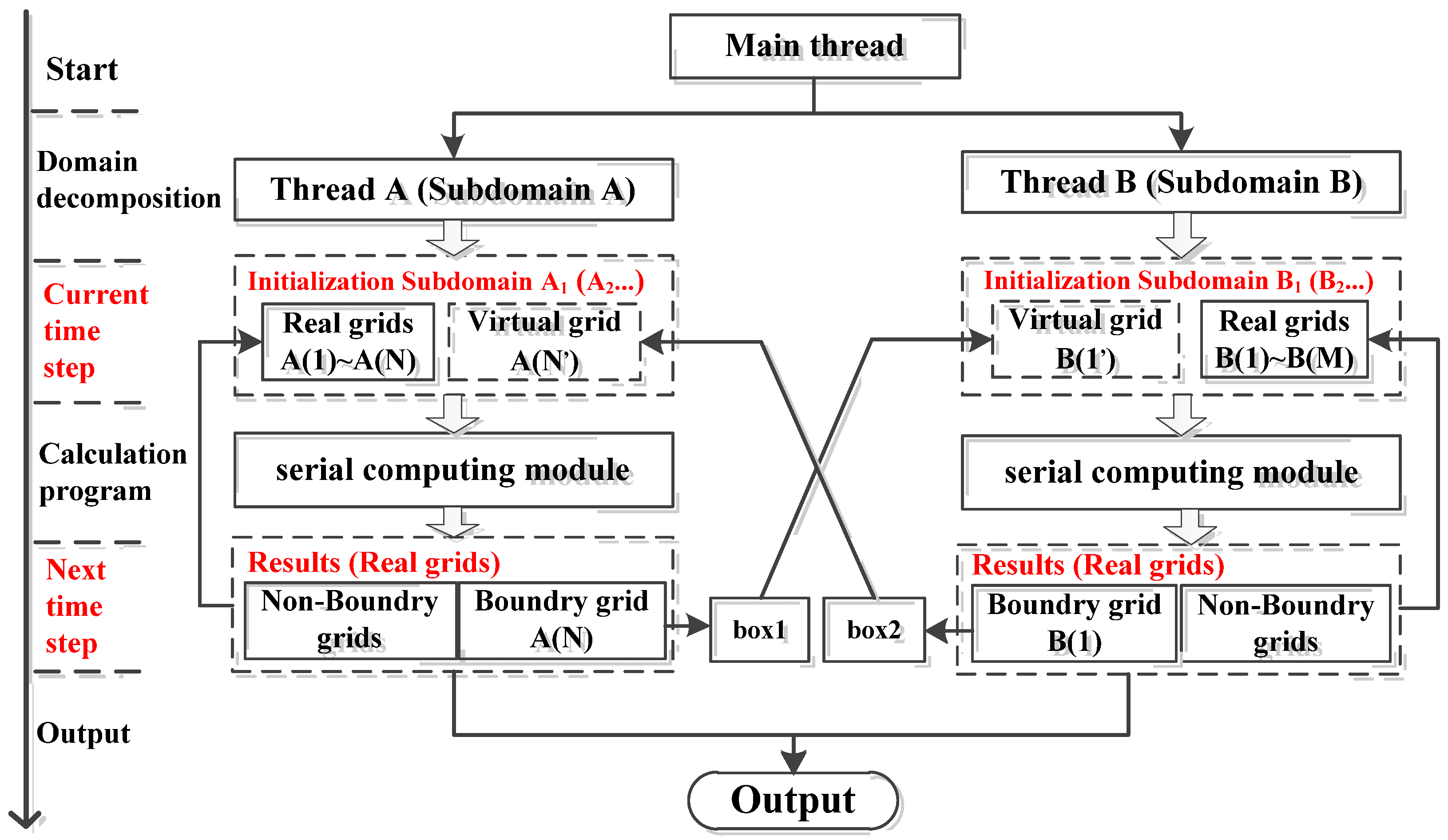
The main thread creates two sub-threads: Thread A and thread B. Both threads are responsible for the computation of Subdomain A and Subdomain B, respectively.

(2)

The main thread creates two containers, box 1 and box 2, as the buffer cache of communication information to facilitate the subsequent thread communication.

(3)

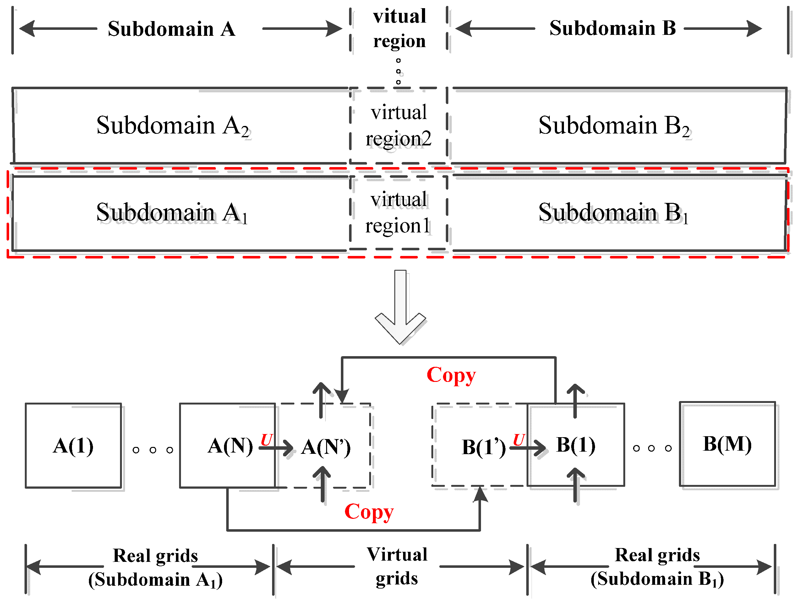
All variables in the subdomains are initialized after each time step begins. The virtual grids are assigned by reading the containers. Take Thread A as an example, where the assignment of virtual grid A(N’) of Subdomain A₁ is achieved by reading box 2. Subdomain A₂, A₃, etc. are processed in a similar way.

(4)

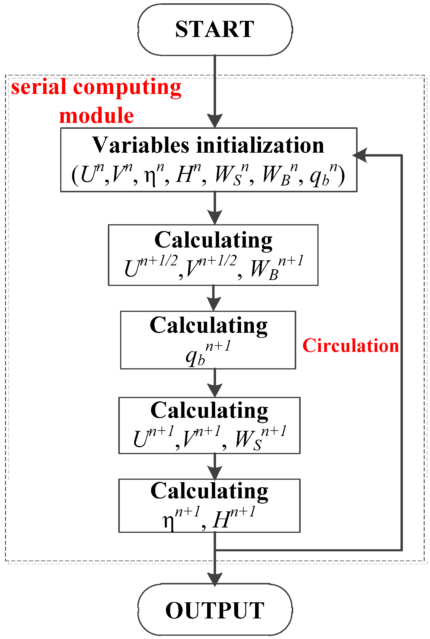
Each sub-thread executes the serial program module (Figure 2) to calculate all the results of the real grids in each subdomain.

(5)

The calculated results of the boundary grids are written to the corresponding containers. Again, take Thread A as an example: The calculated results of A(N) of Subdomain A₁ are written to box 1, thus providing data support to Thread B for the next time step’s computation. Subdomain A₂, A₃, etc. are processed in a similar way.

(6)

Finally, the current computational results are saved and Steps 3–5 are repeated to start the next time step’s computation. The process repeats until all the velocity and water level at each time step in the whole domain have been obtained.

The solution steps of the non-hydrostatic model (parallel computing) are shown in flow chart form in Figure 4.

4.4. Key Techniques and Program Codes

The key techniques involved in the parallel computing method include thread creation, control of the sub-threads by the main thread, and synchronous communication between sub-threads.

“ThreadStart()”, a function in the Windows API Library, can be directly called for thread creation. The main thread should also create two containers, box 1 and box 2, to provide necessary Buffer Cache data for the subsequent thread communication. The main thread commands the sub-threads to perform certain operations via instruction codes specific to the given scenario, such as notifying the sub-thread when reading container data, when writing data to the container, when suspending and waiting for other threads, or when discontinuing the thread. To facilitate the container operations performed by the sub-threads, two state identifiers are also created by the main thread, readerFlag1 and readerFlag2, which are primarily used for judging whether the sub-thread can read from the container or write to the container. The core codes of the main thread are described below.

Box 1. Core Codes of the Main Thread.

static void Main(string[] args)  // main program starts

{

// define a container type (structure)

struct BOX

{

  public double BoxU;  // the type of the stored data is flow velocity U

public double BoxV;  // the type of the stored data is flow velocity V

  public double BoxIta;  // the type of the stored data is water level η

...

}

// two examples of the containers, box1 and box2, are created

BOX box1;

BOX box2;

// two state identifiers are set

bool readerFlag1 = true;  // box1 is readable and not writable when it is true

bool readerFlag2 = true;  // box2 is readable and not writable when it is true

// two sub-threads are created: Thread A and Thread B

Thread A = new Thread (new ThreadStart (ThreadA));

Thread B = new Thread (new ThreadStart (ThreadB));

}

As shown in Figure 4, both threads have two communications within one time step. The first communication occurs during initialization of the variables, and the second occurs after serial program module execution. Synchronous communication between the sub-threads is the key to the success of the parallel computing program. As its name implies, the synchronous communication between sub-threads relates to two major factors: Communication between threads, and communication synchronism. Based on containers (box 1 and box 2) that the main thread creates, communication between threads is achieved via the producer–consumer model. The producer–consumer model is described as follows: The producer creates data of a certain type and stores them in the container; the consumer reads from the container. This will be discussed in greater detail below.

As Figure 4 shows, the next time step’s computation of one sub-thread relies on the previous step’s results of the other sub-thread. As the running speeds of the two sub-threads also differ, bugs may occur if thread communication synchronism cannot be guaranteed. For example, if Thread A is planning to write to box 1 at one point while thread B is reading from box 1, an operation conflict of the container by different sub-threads occurs. To solve the problem, the thread lock technique is utilized to guarantee communication synchronism and avoid repetitive operations of the container executed by various threads. Based on the state identifiers (readerFlag1 and readerFlag2) created by the main thread, the keyword “lock”, the function “Monitor.Wait()”, and the function “Monitor.Pulse()” are used here to realize thread interlocking, thread waiting, and thread notification. Take Thread A’s first communication as an example, where thread A is planning to read from box 2: It first judges whether box 2 is readable based on readerFlag2, and if box 2 is not readable, the function “Monitor.Wait()” allows Thread A to suspend and wait. If box 2 is readable, relevant codes are locked by the keyword “lock” and box 2 is occupied exclusively by Thread A. Thread B is then forced to suspend and wait if also wants to operate box 2. After Thread A has read from box 2 completely, the function “Monitor.Pulse()” is used to remove the thread lock. The status of readerFlag2 is also changed to allow it to notify the other thread in the waiting queue to resume. The sub-thread codes are described below.

Box 2. Core codes of sub-threads (Example: Thread A).

public void ThreadA()

{

// start the initialization of variables as Thread A plans to read from box2

lock (this)        // box2 can only be operated by thread A

 {

  if (!readerFlag2)  // Thread A will suspend and wait if box2 is not readable

  {

     Monitor.Wait(this);

  }

  else   // the box2 is assigned to the virtual grid A(N’) if box2 is readable

  {

    A(N’)_n = box2;  // the box2 is assigned to A(N’) (current time step n)

    readerFlag2 = false;  // readerFlag2 is supposed to be false after reading

    Monitor.Pulse(this);  // relieve occupation of box2 and notify Thread B to resume

  }

 }

Serial.start;        // start to execute serial computing module

// serial computing is completed, result is written to box1

lock (this)       // box1 can only be operated by thread A

 {

  if (readerFlag1)    // Thread A will suspend and wait if box1 is not writable

  {

    Monitor.Wait(this);

  }

  else        // the virtual grid A(N) is assigned to the box2 if box1 is writable

  {

    box1 = A(N)_n + 1;  // A(N’) (next time step n+1) is assigned to the box1

    readerFlag1 = true;  // indicating that box1 is readable

    Monitor.Pulse(this); // relieve occupation and notify Thread B to resume

  }

 }

}

The thread communication and thread lock techniques mentioned above ensure that each sub-thread first reads data from the container once in one time step, then the serial computing module is executed and the results of the boundary grids are written to the corresponding container. No computation of the next time step is performed before the final writing work of the two sub-threads is complete. This guarantees that the parallel computing procedures run in an orderly manner until all computational results are determined. The multithreading parallel computing method proposed in this paper can be implemented on the majority of computers. It maximizes CPU resources and comes with several advantages such as low cost, high feasibility, and high efficiency.

5. Model Verification

The process of wave propagation on an underwater submerged breakwater is very complex. This process was employed to test the performance of the proposed model in simulating high-frequency short wave motion. It is commonly used to verify non-hydrostatic models. The proposed model was used for four experiments on solitary wave propagation over a flat bottom, solitary wave experiment by Madsen [31], sinusoidal wave experiment by Beji [1], and sinusoidal wave experiment by Nadaoka [32]. All parallel programs were executed under double-thread conditions (i.e., with the computational domain divided into two equal parts in the x direction). Comparison between the parallel computing program and serial computing program of the non-hydrostatic model indicated that there is little difference between the computational results under both modes. The maximum deviation is less than 3%. This high consistency may be attributable to the favorable performance of the virtual grid technique. So no further computational results under the serial mode are discussed here; the result of the non-hydrostatic model is simply stated as the computational result under the parallel computing mode due to the similarity between the two. A potential reason for the deviation between the serial and parallel results is the floating point precision issue.

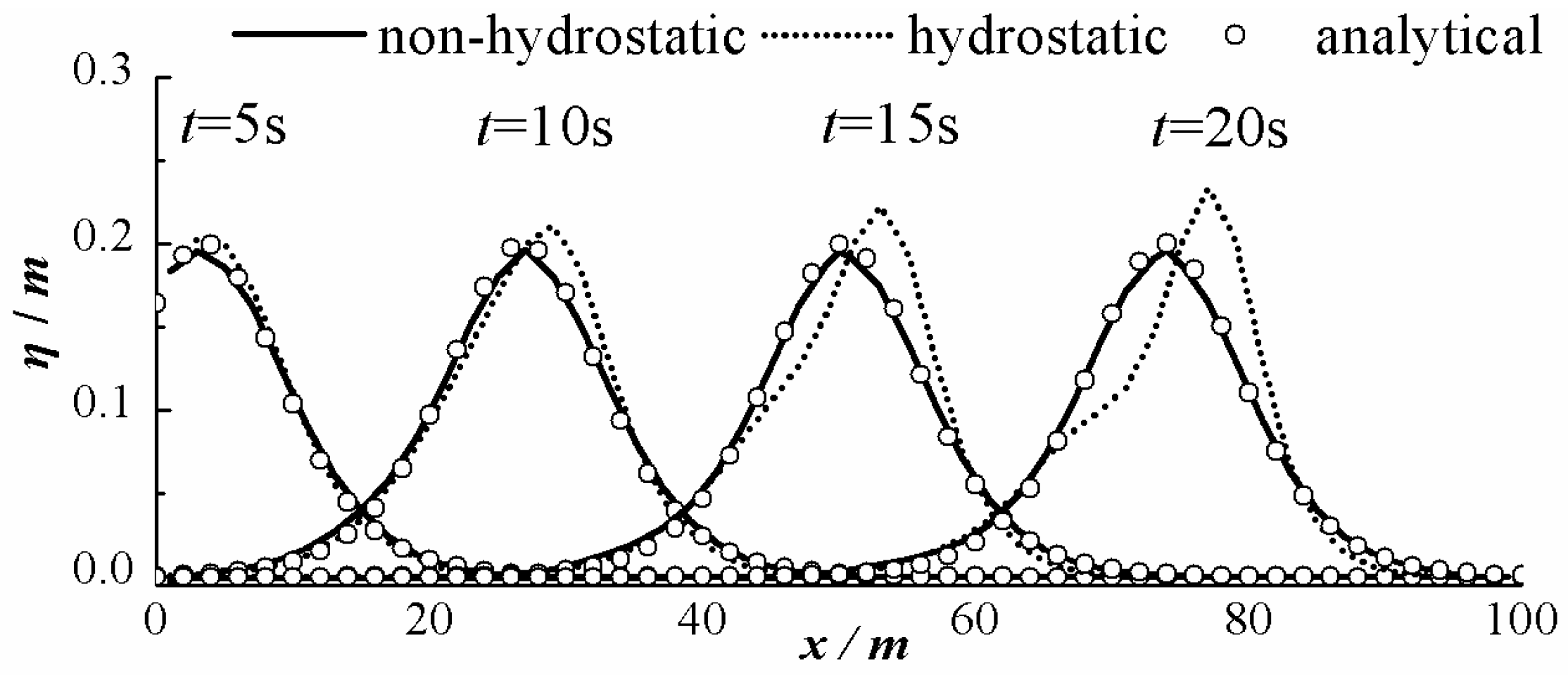
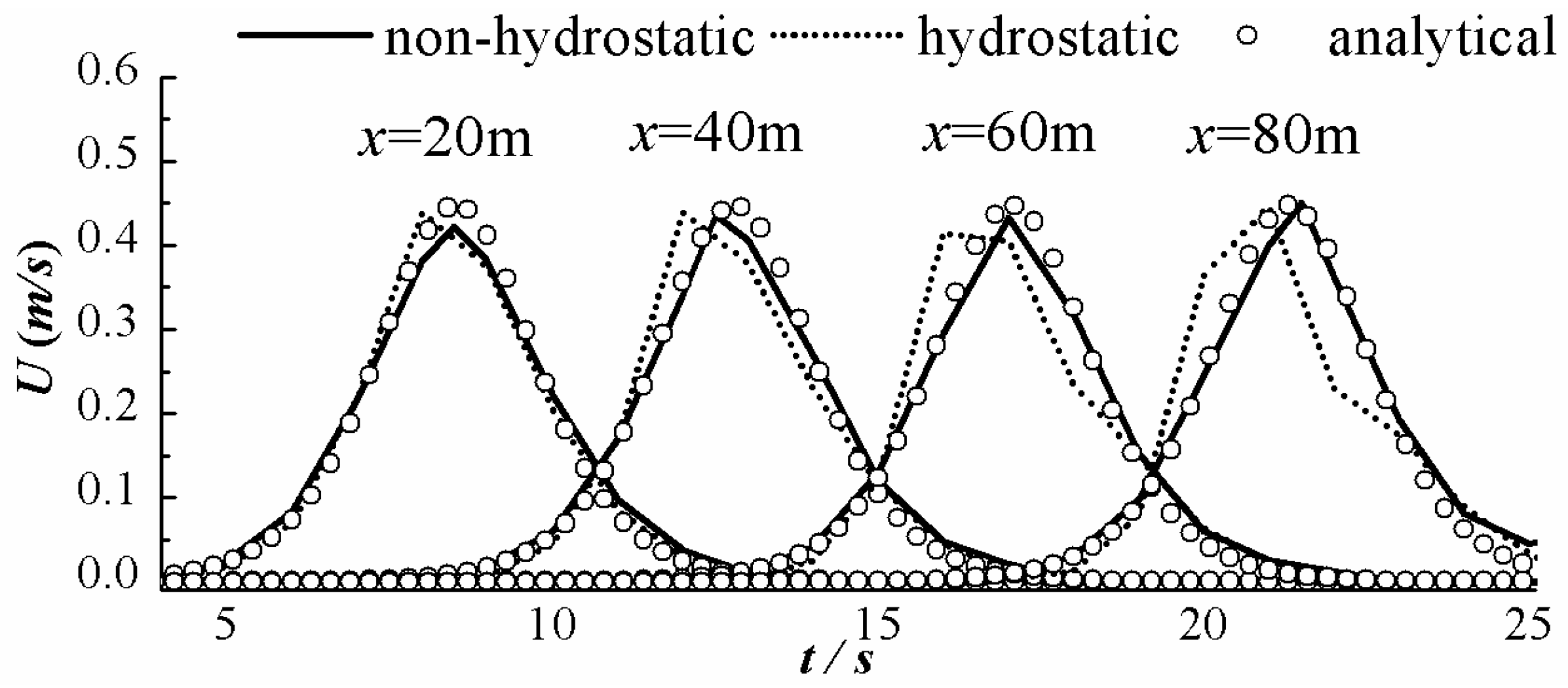
5.1. Solitary Wave Propagation over a Constant Water Depth Channel

When bottom friction and flow viscosity are ignored, the waveform and wave amplitude remain unchanged during solitary wave propagation over a flat bottom. This is accompanied by significant dynamic pressure variation. To test the performance of the model, a 100 m long, 2 m wide, and 2 m deep channel is considered. At the beginning, a solitary wave with the wave amplitude of 0.2 m is at x = −20 m from the left. The simulation time is 30 s; Δx = 2 m; Δy = 1 m; Δt = 0.005 s.

Figure 5 presents the analytical solution of the real waveform and waveforms simulated by the hydrostatic model and non-hydrostatic model at different points in time (t = 5, 10, 15, and 20 s). Figure 6 presents the analytical velocity U and U simulated by the hydrostatic model and non-hydrostatic model at different locations (x = 20, 40, 60, and 80 m). The simulated results of the non-hydrostatic model are in good agreement with the analytical solution, which demonstrates that the non-hydrostatic model can accurately simulate solitary wave propagation over the flat bottom. The simulated results of the hydrostatic model roughly coincide with the analytical solution, however, the simulated value of the wave peak, its occurrence time, and its occurrence position significantly deviate from the analytical solution. The deviation also grows increasingly more significant over time. As shown in Figure 5, the simulated value of the wave peak obtained via hydrostatic model deviates by 25% from the analytical solution when t = 20 s.

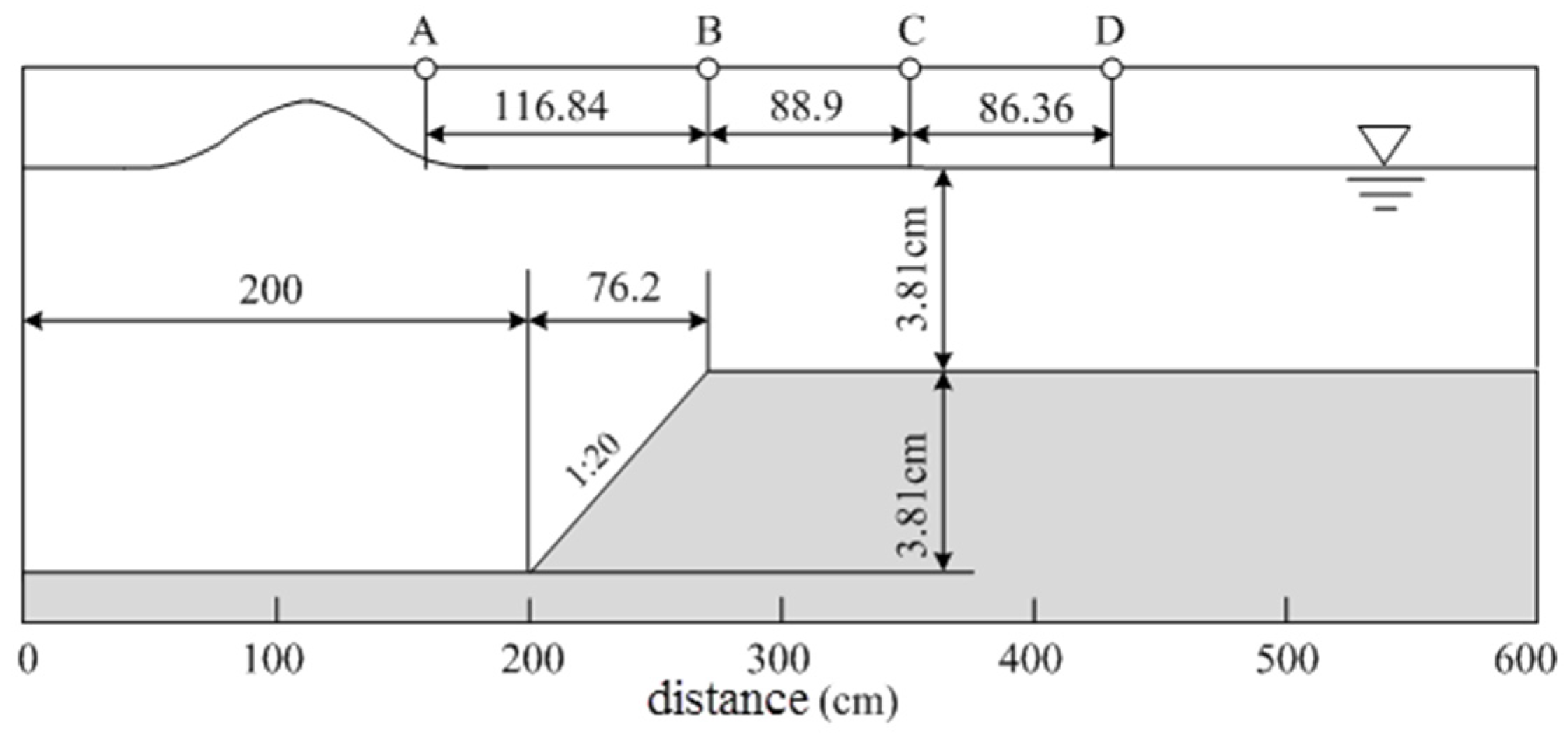
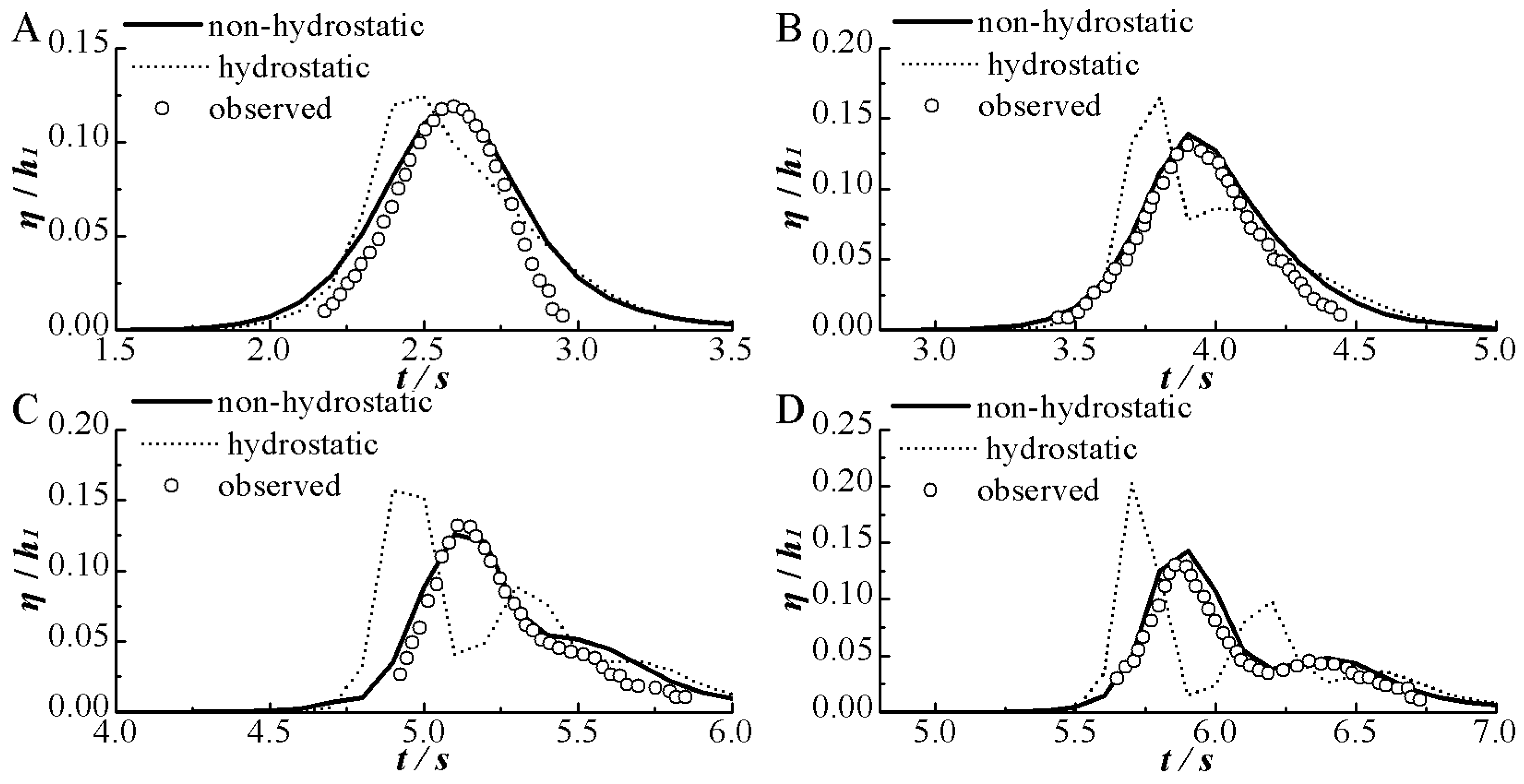
5.2. Madsen’s Solitary Wave Experiment

Madsen made an experimental setup to study the solitary wave shoaling over a submerged bar [31], as shown in Figure 7. There was a slope which was 200 cm far from the left side of the channel. The solitary wave propagates from a constant depth h₁ = 7.62 cm to a smaller constant depth h₂ = 3.81 cm through a slope. There were four stations, A, B, C and D (x = 159.36, 276.2, 365.1, 423.52 cm), observing the free surface. The initial position of the wave crest was at x = −80 cm, and its amplitude was 0.9144 cm. The size of the simulation region is 600 cm and the simulation time is 10 s; Δx = Δy = 5 cm; Δt = 0.001 s.

Figure 8 presents the measured values and the simulated values of the non-hydrostatic and hydrostatic models at four monitoring stations: Stations A, B, C, and D. Oscillation occurs in the hydrostatic simulated results at Stations B, C, and D. The main reason for dispersion is that solitary wave splits into a series of short waves when it is under dynamic pressure. After the short waves pass through these three monitoring stations, decreased dynamic pressure, declined dispersion, and disappeared oscillation occur. Clearly, then, the hydrostatic model cannot correctly simulate the short wave and its dispersion effect as the influence of the dynamic pressure is not considered. The simulated results of the non-hydrostatic model closely coincide with the measured data and the simulated results of the 2D non-hydrostatic model previously developed by the author of this paper [20]. In short, it effectively simulates the process of solitary wave propagation from the abyssal zone to the shoal water.

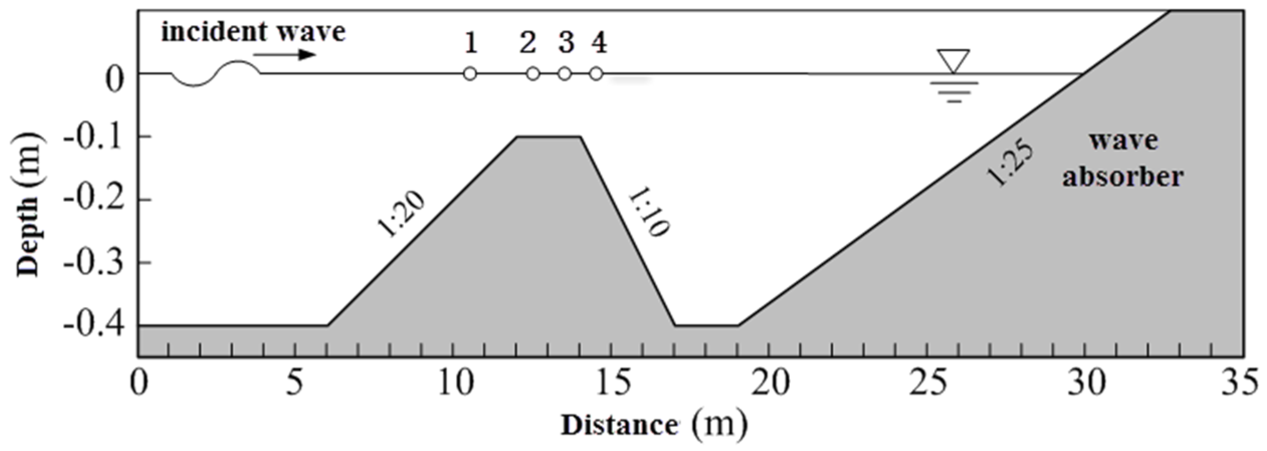
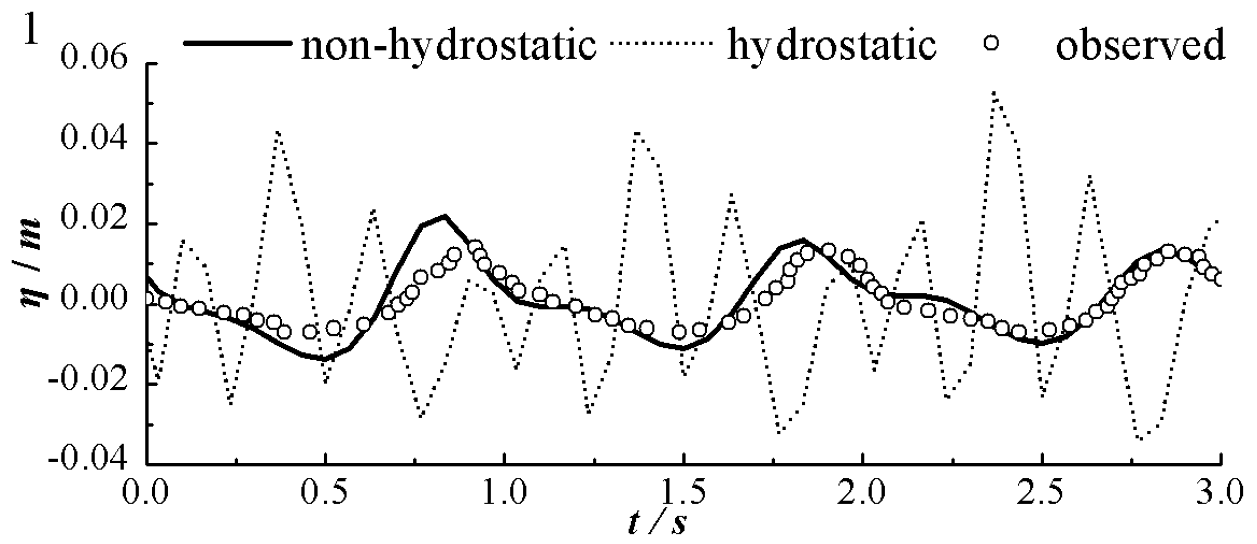
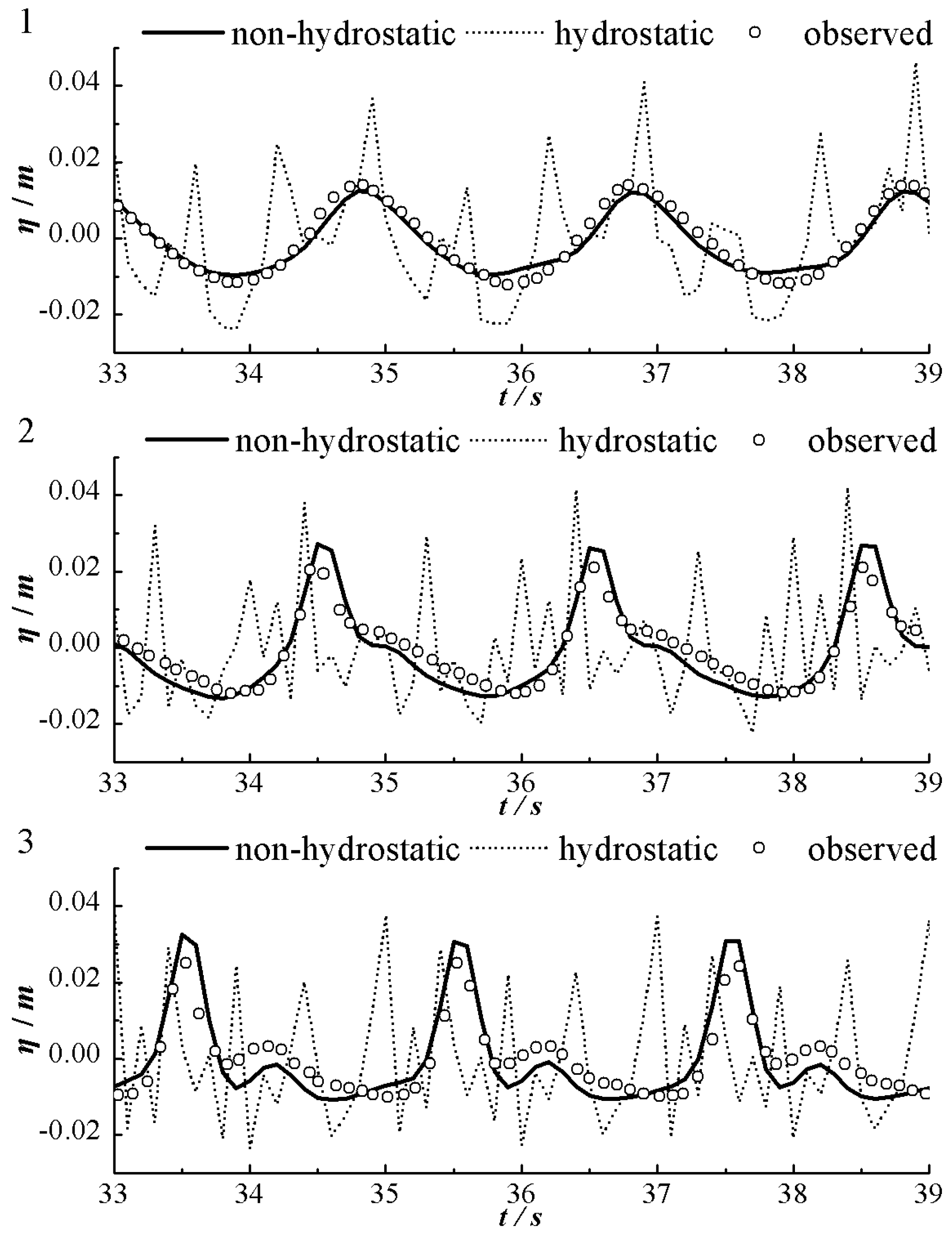
5.3. Beji’s Sinusoidal Wave Experiment

Beji made an experimental setup to study the sinusoidal wave travelling over a submerged bar [1], as shown in Figure 9. The flume is 35 m long, 0.8 m wide, and 0.4 m deep. At the left there was a wave generator making sinusoidal wave trains. Behind the bar, there was a slope as a wave absorber to absorb the waves coming from the left. There were four stations, 1, 2, 3, and 4 (x = 10.5, 12.5, 13.5, 14.5 m), observing the free surface. The sinusoidal wave had a wave amplitude and period of 0.01 m and 2.02 s, respectively. The size of the simulation region is 30 m (x = 0~30 m) and the simulation time is 40 s; Δx = 0.05 m; Δy = 0.1 m; Δt = 0.005 s.

Figure 10 presents the observed water level at Stations 1–4, as well as the simulated results of the non-hydrostatic and hydrostatic models. The simulated value of the hydrostatic model significantly differs from the observed value and violent oscillation occurs in the simulated water level, thus, the simulation is inaccurate. Conversely, the simulated value of the non-hydrostatic model excellently coincides with the observed data, indicating that the non-hydrostatic model proposed in this paper accurately simulates sinusoidal wave propagation along submerged breakwater.

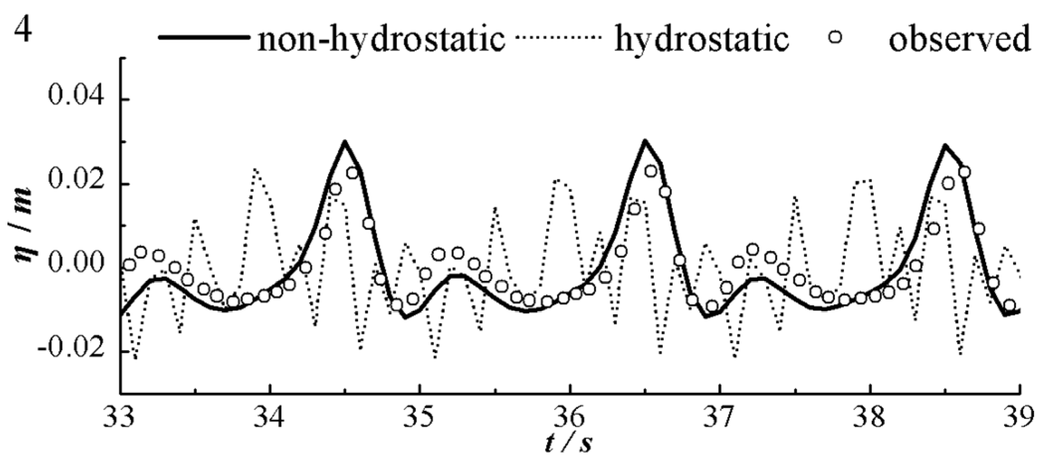
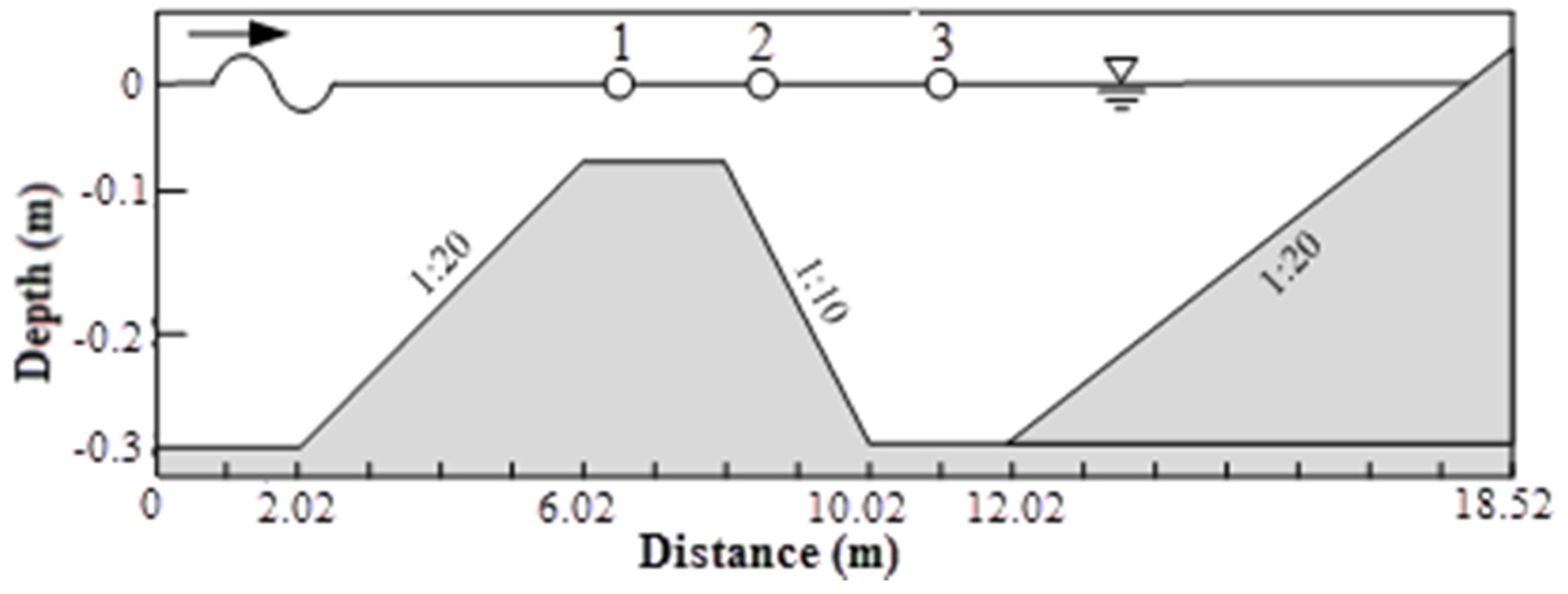
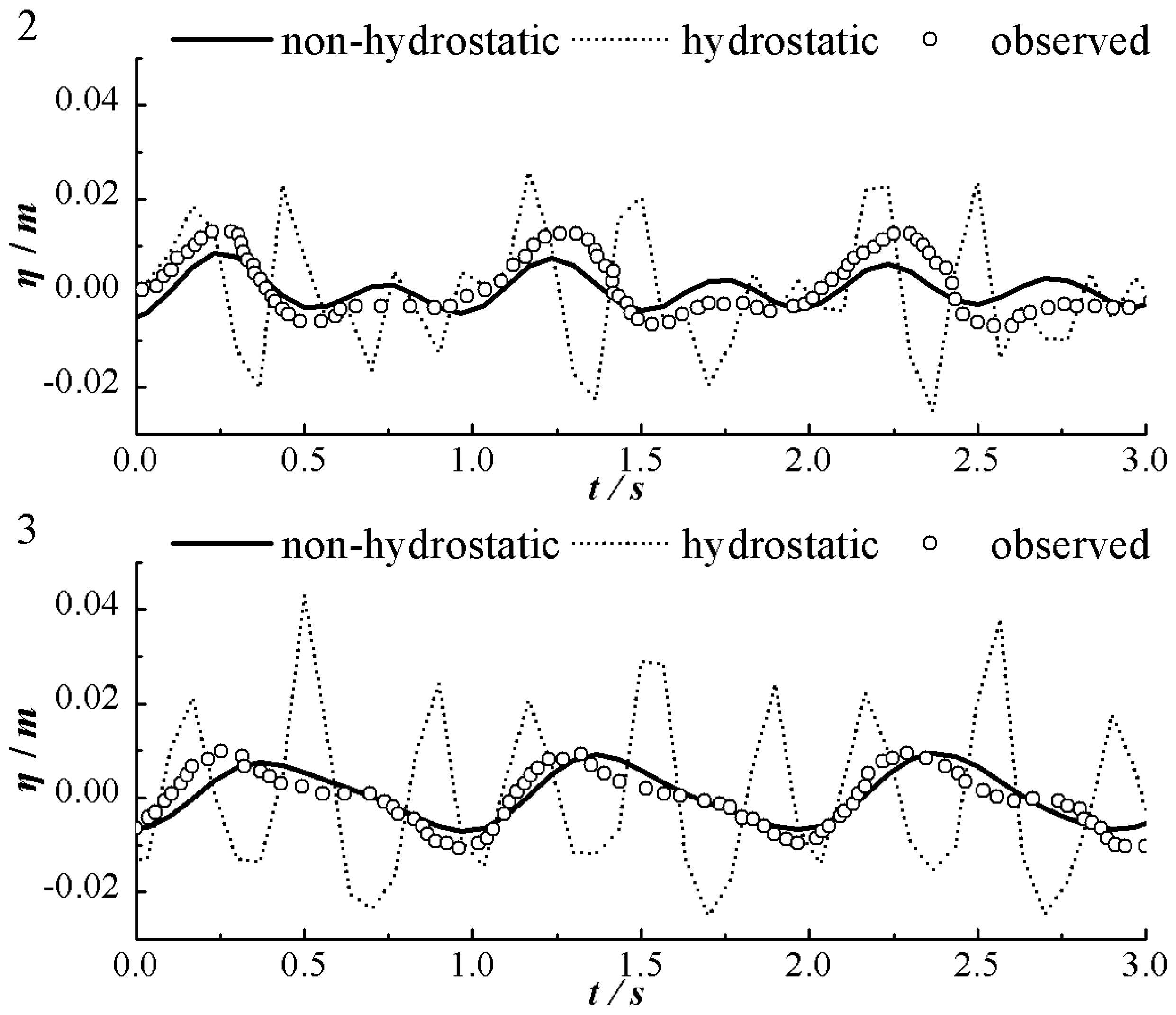
5.4. Nadaoka’s Sinusoidal Wave Experiment

In addition to Beji, Nadaoka made a smaller experimental setup [32], as shown in Figure 11. There was a 18.52 m long and 0.3 m deep channel. At the left was a wave generator making sinusoidal wave trains. Surface elevations were measured at three locations (x = 6.52, 8.52, 11.02 m). The sinusoidal wave had a wave amplitude and period of 0.01 m and 1.5 s, respectively. The size of the simulation region is 12 m (x = 0~12 m); the simulation time is 40 s; Δx = Δy = 0.1 m; Δt = 0.01 s.

Figure 12 presents the measured values of the water level η at three monitoring stations and the simulated η via non-hydrostatic and hydrostatic models. The simulated values of the non-hydrostatic model are in good agreement with the measured values, indicating that the non-hydrostatic model indeed simulates the short wave dispersion generated as the wave passes through an area with abrupt changes in terrain. Compared to the simulated results by the hydrostatic model in Beji’s experiment, more violent oscillation occurs in the simulated η in Nadaoka’s experiment due to the fact that the incident wave in the latter has a shorter period and higher nonlinearity and diffusivity compared to that in the former. More significant simulation distortion occurs in the hydrostatic model, as no dynamic pressure is taken into account.

5.5. Computing Efficiency Analysis

The computational efficiency of the non-hydrostatic model under the parallel computing mode and serial computing mode are compared and analyzed in this section.

Table 1. CPU time of serial computing and parallel computing (four tests).

Test	Time Step (s)	Space Step (m)	Time of Serial Computing (s)	Time of Parallel Computing (s)	1 Increase Rate of Efficiency (%)
5.1	Δt = 0.005	Δx = 1	1.37	0.85	0.38
		Δx = 2	0.72	0.43	0.39
		Δx = 4	0.31	0.22	0.28
5.2	Δt = 0.001	Δx = 0.025	5.42	3.72	0.31
		Δx = 0.05	2.75	1.81	0.34
		Δx = 0.1	1.37	0.89	0.35
5.3	Δt = 0.005	Δx = 0.025	80.12	62.36	0.22
		Δx = 0.05	40.53	31.09	0.23
		Δx = 0.1	22.89	15.64	0.32
5.4	Δt = 0.01	Δx = 0.05	9.25	6.87	0.26
		Δx = 0.1	4.75	3.47	0.27
		Δx = 0.2	2.37	1.69	0.29

¹ Increase rate of efficiency (%): 1 − time of parallel computing/time of serial computing.

presents the CPU time consumed in different experiments under different space and time step combinations based on serial and parallel modes. All programs were run on a PC with Intel i7-4790K CPU 4.0 GHz, 8 GB memory. The codes were compiled with the Visual Studio 2010 IDE (Integrated Development Environment) and C# language.

As shown in Table 1, the parallel computing program saves 20%–40% computation time compared to the serial computing program when other conditions are kept uniform. It demonstrates that the parallel computation method proposed by this paper has higher computational efficiency compared to the conventional serial computing method. To evaluate the computational efficiency of the parallel computing method as systematically as possible, two indexes are introduced: parallel acceleration rate and parallel efficiency. The parallel acceleration rate is defined as S_P = T_s/T_P, where T_s represents the time consumed by the serial computing program and T_P represents the time consumed by joint parallel computation of P threads (P = 2). Parallel efficiency is defined as the ratio of speed-up to the number of threads, E_P = S_P/P. According to the data shown in Table 1, averaged S_P and E_P of the parallel non-hydrostatic program in the four experiments are approximately 1.45 and 72%. In regards to the double threads, the most ideal conditions comprise a speed-up ratio of 2 and parallel efficiency of 100%. It is important to note, however, that communication between threads and waiting consume time during the actual operation of the program. Thus, the actual computational efficiency does not reach the theoretical maximum value.

Table 2. Average CPU time per time step per grid of the four models.

Model	Number of Computational Cores	Average CPU Time per Time Step per Grid (μs)
The proposed model	2	0.73
SWASH	2	0.78
Guo’s model	1	1.68
Zijlema’s model	1	15

presents the average CPU time per time step per grid of four efficient 2D non-hydrostatic hydrodynamic models: The proposed model, SWASH [25], Guo’s model [33] and Zijlema’s model [34]. The SWASH model employs a stripwise grid partitioning method and message passings are implemented by MPI. A so-called wavefront approach has been chosen as the parallelization strategy for the SIP method. The SWASH model was tested on a dedicated Linux cluster with eight nodes, each of which has two dual-core 64-bit AMD processors (1.8 GHz, 4 MB L2 cache). Guo’s model adopts a novel alternating direction implicit scheme to avoid the usage of a complicated iteration method, thus enhancing its calculation efficiency. Guo’s model was carried out on a PC with AMD Athlon 5000+ CPU 2.59 GHZ and 2 GB memory. Zijlema’s model adopts an efficient, preconditioned Krylov subspace technique to solve the discretized Poisson equation; it was tested on a 2.0 GHz Pentium machine.

According to the data shown in Table 2, the proposed model outperforms the other three models. SWASH not only includes a stripwise grid partitioning method (which is similar to the domain decomposition method used here) but also parallelization for SIP (an iteration method) via a wavefront approach. Thus SWASH had a better performance of CPU time than Guo’s model and Zijlema’s model. The CPU time per time step per grid of SWASH model is comparable to ours. But we tested the proposed model on a PC with higher configuration, so the CPU time of the proposed model is slightly smaller than that of SWASH. Guo’s model and Zijlema’s model exploit PPE solutions to minimize computing time, but both were tested on a single-core PC without parallelization. Compared with parallelization technique, mathematics methods have limited effect on efficiency improvement of non-hydrostatic models. Accordingly, their models may be less efficient than the proposed model with parallelization.

6. Conclusions

This paper proposes a comparatively simple parallelization method based on multithreading technique in Windows system for a 2D non-hydrostatic hydrodynamic model. With the pressure divided into hydrostatic and dynamic components, the horizontal momentum equations are obtained by integrating the Navier–Stokes equations from the bottom to the free surface. The vertical momentum equation is approximated by the Keller-box scheme. All the terms except the dynamic pressure gradient term in the horizontal momentum equation are solved explicitly by central difference scheme. The dynamic pressure gradient term is solved by the Crank–Nicolson scheme. A two-step method is used to solve the finite difference equation. A parallel strategy based on block decomposition computation is utilized. The original computational domain is subdivided into two subdomains which are physically connected via a virtual boundary technique. Two sub-threads are created and tasked computation of the two subdomains. The producer–consumer model and the thread lock technique are used to achieve synchronous communication between sub-threads. The validity of the model was verified by solitary wave propagation experiments over a flat bottom and slope, followed by two sinusoidal wave propagation experiments over submerged breakwater. The parallel computing method proposed here was found to effectively enhance computational efficiency and save 20%–40% computation time compared to serial computing. The parallel acceleration rate and acceleration efficiency are approximately 1.45% and 72%, respectively. The parallel computing method proposed in this paper makes a certain contribution to the popularization of non-hydrostatic models. Researchers who have basic programming knowledge can reproduce or modify the proposed method on a computer with minimal memory and hardware. Our method may also benefit those readers who are experts in other water environmental modeling fields (e.g., water temperature models and water quality models), because it is readily extendable other water environmental models. To further improve the computational efficiency of the parallel computing program, future studies are yet warranted to reduce the communication consumption among threads and to achieve expansion from double threads to multiple threads.

References

1. Beji, S.; Battjes, J.A. Experimental investigation of wave propagation over a bar. Coast. Eng. 1993, 19, 151–162. [Google Scholar] [CrossRef]
2. Chang, K.A.; Hsu, T.J.; Liu, P.L.F. Vortex generation and evolution in water waves propagating over a submerged rectangular obstacle Part I. Solitary waves. Coast. Eng. 2001, 44, 13–36. [Google Scholar] [CrossRef]
3. Blenkinsopp, C.E.; Chaplin, J.R. The effect of crest submergence on wave breaking over submerged slopes. Coast. Eng. 2008, 55, 967–974. [Google Scholar] [CrossRef]
4. Peregrine, D.H. Long waves on a beach. J. Fluid Mech. 1967, 27, 815–827. [Google Scholar] [CrossRef]
5. Beji, S.; Battjes, J.A. Numerical simulation of nonlinear wave propagation over a bar. Coast. Eng. 1994, 23, 1–16. [Google Scholar] [CrossRef]
6. Casulli, V.; Stelling, G. Numerical simulation of 3D quasi-hydrostatic, free-surface flows. J. Hydraul. Eng. 1998, 124, 678–686. [Google Scholar] [CrossRef]
7. Zhou, J.G.; Stansby, P.K. An arbitrary Lagrangian-Eulerian σ (ALES) model with non-hydrostatic pressure for shallow water flow. Comput. Method Appl. Mech. Eng. 1998, 178, 199–214. [Google Scholar] [CrossRef]
8. Stelling, G.; Zijlema, M. An accurate and efficient finite-difference algorithm for non-hydrostatic free-surface flow with application to wave propagation. Int. J. Numer. Meth. Fluids 2003, 43, 1–23. [Google Scholar] [CrossRef]
9. Bai, Y.F.; Cheung, K.F. Depth-integrated free-surface flow with a two-layer non-hydrostatic formulation. Int. J. Numer. Meth. Fluids 2012, 69, 411–429. [Google Scholar] [CrossRef]
10. Bai, Y.F.; Cheung, K.F. Depth-integrated free-surface flow with parameterized non-hydrostatic pressure. Int. J. Numer. Meth. Fluids 2013, 71, 403–421. [Google Scholar] [CrossRef]
11. Yuan, H.; Wu, C.H. A two-dimensional vertical non-hydrostatic σ model with an implicit method for free-surface flows. Int. J. Numer. Meth. Fluids 2004, 44, 811–835. [Google Scholar] [CrossRef]
12. Yuan, H.; Wu, C.H. An implicit three-dimensional fully non-hydrostatic model for free-surface flows. Int. J. Numer. Meth. Fluids 2004, 46, 709–733. [Google Scholar] [CrossRef]
13. Namin, M.M.; Lin, B.; Falconer, R.A. An implicit numerical algorithm for solving non-hydrostatic free-surface flow problems. Int. J. Numer. Meth. Fluids 2001, 35, 341–356. [Google Scholar] [CrossRef]
14. Guo, C.; Chen, X.; Vlasenko, V.; Stashchuk, N. Numerical investigation of internal solitary waves from the Luzon Strait: Generation process, mechanism and three-dimensional effects. Ocean Model. 2011, 38, 203–216. [Google Scholar] [CrossRef]
15. Shen, C.Y.; Evans, T.E.; Oba, R.M.; Finette, S. Three-dimensional hindcast simulation of internal soliton propagation in the Asian Seas International Acoustics Experiment area. J. Geophys. Res. 2009, 114, C01014. [Google Scholar] [CrossRef]
16. Yuan, H.; Wu, C.H. Fully nonhydrostatic modeling of surface waves. J. Eng. Mech. 2006, 132, 447–456. [Google Scholar] [CrossRef]
17. Bai, Y.; Cheung, K.F. Dispersion and nonlinearity of multi-layer non-hydrostatic free-surface flow. J. Fluid Mech. 2013, 726, 226–260. [Google Scholar] [CrossRef]
18. Young, C.C.; Wu, C.H.; Liu, W.C.; Kuo, J.T. A higher-order non-hydrostatic σ model for simulating non-linear refraction–diffraction of water waves. Coast. Eng. 2009, 56, 919–930. [Google Scholar] [CrossRef]
19. Stelling, G.; Busnelli, M. Numerical simulation of the vertical structure of discontinuous flows. Int. J. Numer. Meth. Fluids 2001, 37, 23–43. [Google Scholar] [CrossRef]
20. Guo, X.; Kang, L.; Jiang, T. A new depth-integrated non-hydrostatic model for free surface flows. Sci. China Technol. Sci. 2013, 56, 824–830. [Google Scholar] [CrossRef]
21. Jankowski, J.A. Parallel implementation of a non-hydrostatic model for free surface flows with semi-Lagrangian advection treatment. Int. J. Numer. Meth. Fluids 2009, 59, 1157–1179. [Google Scholar] [CrossRef]
22. Hérault, A.; Bilotta, G.; Dalrymple, R.A. SPH on GPU with CUDA. J. Hydraul. Res. 2010, 48, 74–79. [Google Scholar] [CrossRef]
23. Bleichrodt, F.; Bisseling, R.H.; Dijkstra, H.A. Accelerating a barotropic ocean model using a GPU. Ocean Model. 2012, 41, 16–21. [Google Scholar] [CrossRef]
24. Nesterov, O. A simple parallelization technique with MPI for ocean circulation models. J. Parallel Distrib. Comput. 2010, 70, 35–44. [Google Scholar] [CrossRef]
25. Zijlema, M.; Stelling, G.; Smit, P. SWASH: An operational public domain code for simulating wave fields and rapidly varied flows in coastal waters. Coast. Eng. 2011, 58, 992–1012. [Google Scholar] [CrossRef]
26. Keulegan, G.H.; Patterson, G.W. Mathematical theory of irrotional translation waves. J. Res. Natl. Bur. Stand. 1940, 24, 47–101. [Google Scholar] [CrossRef]
27. Orlanski, I. Simple boundary-condition for unbounded hyperbolic flows. J. Comput. Phys. 1976, 21, 251–269. [Google Scholar] [CrossRef]
28. Keller, H.B. A new difference scheme for parabolic problems. In Numerical Solutions of Partial Differential Equations II; Hubbard, B., Ed.; Academic Press: New York, NY, USA, 1971; pp. 327–350. [Google Scholar]
29. Yamazaki, Y.; Kowalik, Z.; Cheung, K.F. Depth-integrated, non-hydrostatic model for wave breaking and run-up. Int. J. Numer. Meth. Fluids 2009, 61, 473–497. [Google Scholar] [CrossRef]
30. Yorsef, S. Iterative Methods for Sparse Linear Systems, 2nd ed.; SIAM Publications: Philadelphia, PA, USA, 2003. [Google Scholar]
31. Madsen, O.S.; Mei, C.C. The transformation of a solitary wave over uneven bottom. J. Fluid Mech. 1969, 39, 781–791. [Google Scholar] [CrossRef]
32. Nadaoka, K.; Beji, S.; Nakagawa, Y. A fully-dispersive nonlinear wave model and its numerical solutions. In Proceedings of the International Conference on Coastal Engineering, Kobe, Japan, 23–28 October 1994; pp. 427–441.
33. Guo, X.; Kang, L. Depth-integrated, non-hydrostatic model using a new alternating direction implicit scheme. J. Hydraul. Res. 2013, 51, 368–379. [Google Scholar]
34. Zijlema, M.; Stelling, G.S. Further experiences with computing non-hydrostatic free-surface flows involving water waves. Int. J. Numer. Meth. Fluids 2005, 48, 169–197. [Google Scholar] [CrossRef]
Figure 1. Layout of variables.
Water 09 00184 g001
Figure 2. Solution steps of the non-hydrostatic model (serial computing).
Water 09 00184 g002
Figure 3. Domain decomposition and variable assignment of virtual grids.
Water 09 00184 g003
Figure 4. Solution steps of the non-hydrostatic model (parallel computing).
Water 09 00184 g004
Figure 5. Simulated waveform by the non-hydrostatic (solid line) and hydrostatic model (dotted line); analytical waveform (circled) at different points in time (t = 5, 10, 15, and 20 s).
Water 09 00184 g005
Figure 6. Simulated velocity U by the non-hydrostatic (solid line) and hydrostatic model (dotted line); experimental data (circled) at different locations (x = 20, 40, 60, and 80 m).
Water 09 00184 g006
Figure 7. Sketch of the experiment setup of Madsen.
Water 09 00184 g007
Figure 8. Simulated η/h1 by the non-hydrostatic (solid line) and hydrostatic model (dotted line); experimental data (circled) from Stations A, B, C, and D.
Water 09 00184 g008
Figure 9. Sketch of the experimental setup of Beji.
Water 09 00184 g009
Figure 10. Simulated η by the non-hydrostatic (solid line) and hydrostatic model (dotted line); experimental data (circled) from Stations 1–4.
Water 09 00184 g010aWater 09 00184 g010b
Figure 11. Sketch of the experimental setup of Nadaoka.
Water 09 00184 g011
Figure 12. Simulated η by the non-hydrostatic (solid line) and hydrostatic model (dotted line); experimental data (circled) from Stations 1–3.
Water 09 00184 g012aWater 09 00184 g012b