Article

Multivariate Analysis of Joint Probability of Different Rainfall Frequencies Based on Copulas

State Key Laboratory of Simulation and Regulation of Water Cycle in River Basin, China Institute of Water Resources and Hydropower Research, Beijing 100038, China
*
Author to whom correspondence should be addressed.
Water 2017, 9(3), 198; https://doi.org/10.3390/w9030198
Submission received: 30 December 2016 / Revised: 25 February 2017 / Accepted: 6 March 2017 / Published: 9 March 2017

Abstract

:
The performance evaluation of a city’s flood control system is essentially based on accurate storm designs, where a particular challenge is the development of the joint distributions of dependent rainfall variables. When it comes to the research design for consecutive rainfall, the analytical investigation is only focused on the maximum of consecutive rainfalls, and it does not consider the probabilistic relations between the first day of rainfall and the overall rainfall included in consecutive rainfall events. In this study, the copula method is used to separate the dependence structure of multi-day rainfall from its marginal distribution and analyse the different impacts of the dependence structure and marginal distribution on system performance. Three one-parameter Archimedean copulas, including the Clayton, Gumbel, and Frank families, are fitted and compared for different combinations of marginal distributions that cannot be rejected by statistical tests. The fitted copulas are used to generate rainfall events for a system performance analysis, including the conditional probability and design values for different return periods. The results obtained in this study highlight the importance of taking into account the dependence structure of one-day and multi-day rainfall in the context of storm design evaluations and reveal the different impacts of the dependence structure and the marginal distributions on the probability.

1. Introduction

Flooding in most cities is caused by rainstorms. Using rainstorm data is an indirect way to ascertain the design flood compared with the estimate based on discharge data. However, the discharge series in survey regions is often too short to ascertain the design flood directly, since rainfall detection is a relatively systematic process and the data sequence is long and complete [1]. Therefore, hydrological analysis is usually carried out on the basis of rainfall, so as to provide a basis for determining water supply. In general, rain can be represented by such characteristics as precipitation, rainfall intensity and rainfall duration [2]. At present, the analysis of torrential rain generally uses the design rainfall method, which is a univariate analysis based on precipitation (e.g., the designed maximum one-day precipitation and maximum three-day precipitation). In recent years, researchers realized that the analysis of torrential rain based on the distribution of univariate extremum has certain restrictions [3]. Thus, they are trying to analyze the correlation between different characteristics of rainstorms by using multivariable joint distribution, with a view to providing a more comprehensive description of rainstorm events.
Many approaches have been developed to analyse the frequency of design rainfall in a city’s flood control system, such as analytical probability methods [4], Bayesian methods [5], first-order reliability methods [6], and imprecise probability methods [7]. In these methods, the historical rainfall series available are separated into rainfall events, and the probability distributions of some rainfall variables are then used to characterise the stochastic nature of the rainfall. For example, rainfall depth and duration are often used in the literature [8,9,10]. However, when it comes to the research design for consecutive rainfall, the analytical investigation is only focused on the maximum amount of consecutive rainfall, and it does not consider the probabilistic relations between the first day of rainfall and the overall rainfall included in consecutive rainfall events. The features of consecutive rainstorms are analysed in terms of the first day of rainfall and the overall rainfall.
There is increasing attention being given to the use of copulas as a flexible tool to quantify the dependence structure between correlated variables in the fields of hydrology and water engineering [11,12,13]. The use of copulas enables the ability to model the probabilistic dependence structure independently of marginal distributions, allowing for multivariate random events to be described using different types of marginal distributions [14]. This represents a significant advantage compared to conventional multivariate analysis, as many variables of hydrological phenomena cannot be described using the same type of probability distributions. [15] An important application of copulas is modelling the stochastic nature of rainfall and flooding using historical data [16]. Copulas also provide a convenient way to generate samples of correlated rainfall variables, meaning they can be used for flood frequency analysis in conjunction with the Monte Carlo simulation method [17].
In this study, three-day rainfall events and seven-day rainfall events were selected as the samples to research, expressed as three-day and seven-day rainfall, with the first day of rainfall counted as one-day rainfall. The dependence between the first day to the third day of rainfall and the first to the seventh day of rainfall are represented using Archimedean copulas. The copula method is demonstrated using conditional probability to design storms for different return periods. The results show both the suitability and flexibility of the use of Archimedean copulas in simulating the dependence and the significant impacts of the dependence structure on the performance of designed storms on a city’s flood control system.

2. Data and Method

2.1. Methodology

2.1.1. Concept of Copulas

Copulas can be used as multivariate cumulative distribution with standard uniform marginal distributions and represent the dependence structure of random variables. For two random variables X and Y, their marginal cumulative distribution functions are represented as:
u = F X ( x )   and   v = F Y ( y )
H X Y ( x , y ) = C ( u , v )
where u and v are random variables, C ( u , v ) is called a copula and can be uniquely determined when u and v are continuous. It is easy to see that a copula is actually a multivariate distribution function with a uniform marginal distribution [18]. The marginal distributions can be determined by different distributions, and the dependence structures are separated from the marginal distributions [19]. For this, complex multivariate distributions can be built to model stochastic phenomena, such as rainfall, without requiring a better understanding of the marginal distributions. There are many families of copulas that represent different dependence structures [20]. One-parameter Archimedean copulas are of special interest for hydrologic analyses, and the general expression of Archimedean copulas can be written as:
C ( u , v ) = φ 1 ( φ ( u ) + φ ( v ) )
where φ is a convex decreasing function defined in [0,1], satisfying φ ( 1 )   =   0   . and lim t 0 φ ( t ) = . Different forms of the function φ represent different families of Archimedean copulas, for example, the Gumbel, Frank and Clayton families. These copulas can describe a wide range of dependence levels, from negative to positive, and have been used to describe rainfall characteristics in previous studies [21,22]. These are selected to describe the relationship between one-day rainfall and multi-day rainfall in this study. The formulas of Gumbel, Frank and Clayton are as follows:
Gumbel :   C ( u 1 , u 2 ) = exp ( [ ( ln u 1 ) θ + ( ln u 2 ) θ ] 1 θ )
Frank :   C ( u 1 , u 2 ) = 1 θ ln ( 1 + ( e θ u 1 1 ) ( e θ u 2 1 ) e θ 1 )
Clayton :   C ( u 1 , u 2 ) = max [ ( u 1 θ + u 2 θ 1 ) 1 θ , 0 ]
where u 1 and u 2 are random variables.

2.1.2. Copula Fitting

For Archimedean copulas, the simplest method to estimate the parameter θ is through a concordance measurement using Kendall’s τ, which is a rank correlation coefficient that examines the orderings of two measured quantities. The relationship between the parameter θ and Kendall’s τ exists for the Gumbel, Frank and Clayton families [23]. In addition to the non-parametric methods described above, there are some parametric methods available for parameter estimation, such as the conventional Maximum Likelihood (ML) method, the Inference Function for Margins (IFM) method [24], the Canonical Maximum Likelihood (CML) method [25], and the Minimum Distance Methods. The IFM method was used in this study, as it has a better performance compared to the others based on our preliminary tests. More importantly, it allows the exploration of the impacts of the choice of the parametrically estimated marginal Cumulative distribution on copula fitting, as prior research has shown that a number of marginal Cumulative distributions may not be rejected for rainfall variables under several statistical tests [26,27]. The root mean square error is an indicator of the goodness of fit, and it can be calculated as:
RMSE = 1 n i = 1 n { C ( u i , v i ) C n ( u i , v i ) } 2 ,
where C n is the empirical copula. For this measurement, the smaller the values, the better the copula fits the data. Formal hypothetical tests are increasingly used to evaluate the goodness-of-fit for different copulas [28,29]. The Cramér-von Mises statistic is chosen to compare an estimated copula C with the empirical copula C n :
T n = i = 1 n { C ( u i , v i ) C n ( u i , v i ) } 2 .
Higher p-values are desired, as they represent better suitability for the chosen copulas [30,31].
The tail dependence analysis is critical to investigating the magnitude of dependence in the upper and lower tails of a bivariate distribution [32]. It also helps to identify the most suitable copula by emphasising the joint occurrence of extreme values [33]. The tail dependence can be represented by a coefficient. For the Gumbel copula, the upper tail dependence coefficient is:
λ U = 2 2 1 θ
In this study, the following estimator proposed by Frahm was used for non-parameters calculation. The formula is:
λ U = 2 2 exp [ 1 n i = 1 n log ( log 1 u i log 1 v i log 1 max ( u i , v i ) 2 ) ]
where ( u i , v i ) are random, generated from copulas.

2.1.3. Recurrence Interval

The recurrence interval can reflect the risk of variables directly. There are different return periods of two variables events [34]; here, the conditions return period and joint return period were used to calculate the value of one-day rainfall and multi-day rainfall; the joint return period is:
T ( x 1 , x 2 ) = 1 1 + C ( F ( x 1 ) , F ( x 2 ) ) F ( x 1 ) F ( x 2 )
The conditions return period used here is:
T ( X 2 x 2 | X 1 x 1 ) = 1 F ( x 1 ) 1 + C ( F ( x 1 ) , F ( x 2 ) ) F ( x 1 ) F ( x 2 )

2.2. Catchment and Data

2.2.1. The Catchment

In this paper, the Qinhuai River basin (approximately lat 32°2′ N and long 118°78′ E) is selected as the studied catchment. The Qinhuai River basin is located downstream of the Yangtze River, which is in the southwestern part of Jiangsu Province, with a total area of 2658 km2. The region where it is located ranges from the northern subtropics to mid-subtropical. The long-term annual air temperature is 15.4 °C, and the annual range of air temperatures can reach as high as 40 °C. The topography mainly contains plains, hills and mountains. The highest mountain’s altitude is greater than 2400 m. The annual average sunshine time is 2240 h, and the annual average precipitation is 1047.8 mm. The location of the study area, together with the distribution of the meteorological stations used in this study, is shown in Figure 1.

2.2.2. Rainfall Data

Daily rainfall data from twenty-one rain stations were used in this research. The distribution of the twenty-one stations is shown in Figure 1. Because of the material conditions and distribution of these stations, different stations were used to calculate the rainfall of the area using the Thiessen polygon method for different years. Here, the fifteen stations are the Qinhuai new river sluice, Wudingmen Sluice, Chishan New Sluice, Tiansheng Bridge Sluice, Qianhan Village, East Mountain, Jurong, Zhaocun Reservoir, Anjishan Reservoir, North Mountain Reservoir, Ershengqiao Reservoir, Maoshan Reservoir, Fangbian Reservoir, Wolongshan Reservoir, and Zhongshan Reservoir, and they were used to obtain the area rainfall for the years from 2000 to 2010. Fifteen stations, including the Qinhuai New River Sluice, Wudingmen Sluice, Chishan New Sluice, Tiansheng Bridge Sluice, Qianhan Village, East Mountain, Jurong, Zhaocun Reservoir, Anjishan Reservoir, Qinlin, Linchang, Tingzi, Xixie, Tianwang, and Aiyuan, were used to obtain the area rainfall for the years from 1960 to 1999. Five stations, including the East Mountain, Jurong, Anjishan Reservoir, Tiansheng Bridge Sluice, and Tianwang, were used to obtain the area rainfall for the years from 1953 to 1959. All the date series about these stations were shown in Table 1. To study the relationship between one-day area rainfall and multi-day area rainfall for an urban catchment, all the rainfall events with a duration of three days were separated by the first day of rainfall and the total three-day rainfall, and the events with a duration of seven days were separated by the first-day rainfall and the total seven-day rainfall. To guarantee that an individual event was not affected by any other event, the time interval of two time-adjacent events is one day to ensure every daily rainfall event is independent. A total of 1980 events and 1345 events were identified from the rainfall series to study the relationship between the daily area and three-day area rainfall and the seven-day area rainfall. The events with an amount of 4 mm cannot generate flooding, so the events which are less than 4 mm are not considered for analysis in the research. This reduced the number of events to 1307 three-day rainfall and 714 seven-day rainfall events, respectively.

3. Results and Discussion

3.1. Data Analysis

Figure 2 shows scatter plots for the 1307 events with marginal histograms for one-day area and three-day rainfall and 714 events with marginal histograms for one-day area and seven-day rainfall. There is a high frequency of low one-day rainfall, with approximately 50% of the rainfall events having a very small depth of less than 12 mm. For the daily and three-day rainfall events and the daily and seven-day rainfall events, the average daily rainfall is both approximately 16.55 mm, but the maximum is as much as 177.3 mm. Similarly, both the three-day and seven-day rainfall have a high frequency of low rainfall, although approximately 10% have a rainfall greater than 150 mm for three-day rainfall and greater than 190 mm for seven-day rainfall. The average three-day rainfall is 28.61 mm, with a maximum of 242.1 mm. However, the average seven-day rainfall is 43.5 mm, with a maximum of 354.2 mm. The two variables are related to some extent, with a Kendall’s τ = 0.41 for one-day to three-day rainfall and τ = 0.36 for one-day to seven-day rainfall. As seen from the marginal histograms, the two variables do not follow the same marginal distribution. This clearly demonstrates the need to separate the marginal distributions and the dependence structure in the joint distribution for the two series so that the marginal distributions may be simulated by different types of distributions.

3.2. Marginal Distributions

According to previous studies [35], the Generalized Extreme Value (GEV), Generalized Pareto (GP), Log–log and Gamma methods are used to fit the daily rainfall and multi-day rainfall. These functions are fitted using the maximum likelihood estimation method that maximises the log-likelihood function. In the calculation, the maximum number of iterations is specified to be 100, and the accuracy of the estimation is set to 1.0 × 10³.
Three goodness-of-fit tests, including the Kolmogorov-Smirnov (K–S), Anderson Darling (A–D) and Chi-square (ƛ2) tests, are considered here to determine if the data follow one of the specified distributions (the null hypothesis H0). In our study, Kolmogorov-Smirnov (K–S) was selected to test if the data follow one of the specified distributions well. The hypothesis is evaluated at the 0.05 significance level. The critical values of K-S at this level are 0.038 for the daily area rainfall and the three day area rainfall and 0.051 for the daily area rainfall and the seven day area rainfall. Larger statistical values indicate a worse fit to the data. The hypothesis regarding a specific distribution is rejected at the significance level if the test statistic is greater than the relevant critical value given above.
The K–S statistics for one-day, three-day and seven-day rainfall are provided in Table 2 and Table 3. The p-values measure the amount of information against the null hypothesis H0 and are also provided here. The smaller the p-values, the more evidence we have against H0. For the series of one-day and three-day rainfall, the four distributions of one-day rainfall, i.e., GEV, Gamma, Log-Log and Gamma, cannot be rejected with K–S tests and have a decreasing ranking according to the statistical values. However, for three-day rainfall, the GP distribution performs best, followed by Log-Log, GEV and Gamma. Similarly, for the series of one-day and seven-day rainfall, GEV and GP are the best distribution for one-day and seven-day, respectively, while GP and Gamma are the worst distributions for one-day and seven-day, respectively. None of the three distributions can be rejected based on K-S tests. In many cases, it is not possible to determine one single best distribution, particularly when a relatively short series of data is available [36]. All of the three distributions are used to investigate the bivariate distribution using copulas.

3.3. Dependence Structure

The selected marginal distributions for one-day and multi-day rainfall are used to fit the Archimedean copulas using the CML method. Two methods are used to determine the value of θ. For one-day and three-day rainfall, the parametrically estimated values of parameter θ are provided in Table 4, along with their 95% confidence intervals. The values for the Gumbel, Frank and Clayton copulas determined using the non-parametric method are 1.385, 2.592 and 0.701, respectively, from the connection between θ and τ. The parametric estimates for the Gumbel and Frank copulas are in good agreement with those from the non-parametric method and are in the relevant 95% confidence intervals. However, for the Clayton copula, the non-parametric estimate is significantly larger and is outside the 95% confidence interval. This is possibly because the rainfall data shown in Figure 2 illustrate greater dependence in the upper tail than in the lower tail. In contrast, the Clayton copula places more attention on the lower tail than the upper tail. The Gumbel copula is an asymmetric Archimedean copula with a greater dependence in the upper tail than in the lower tail. The Frank copula is a symmetric Archimedean copula. Thus, these two copulas are more appropriate for describing the dependence structure between one-day and three-day rainfall.
The same conclusion is applicable to one-day and seven-day rainfall, with the parametrically estimated values for parameter θ provided in Table 5 along with their 95% confidence intervals. The values for the Gumbel, Frank and Clayton copulas using the parametric method are 1.108, 2.203 and 0.567, respectively. Gumbel and Frank copulas are appropriate for describing the dependence structure between one-day and seven-day rainfall.
Table 6 and Table 7 show the resulting RMSE and Cramér-von Mises statistical values. For the series of one-day rainfall and three-day rainfall, GEV distribution does not have the best performance in the terms of copula fitting when Gamma has the best, although the GEV distribution is the best in terms of the marginal distribution fitting according to the statistics. However, GP is the best three-day distribution and also has good performance in copula fitting; besides, when Log-Log is selected as one-day, Log-Log is better than GP as the three-day distribution. The same conclusion can be drawn from another series. This implies that it is important to consider the goodness-of-fit of both the marginal distributions and the copulas to achieve the best overall performance when constructing a joint distribution of multiple variables. For the three distributions for multi-day rainfall, there are no significant differences in the copula fittings. The Gumbel and Frank copulas are in good agreement.
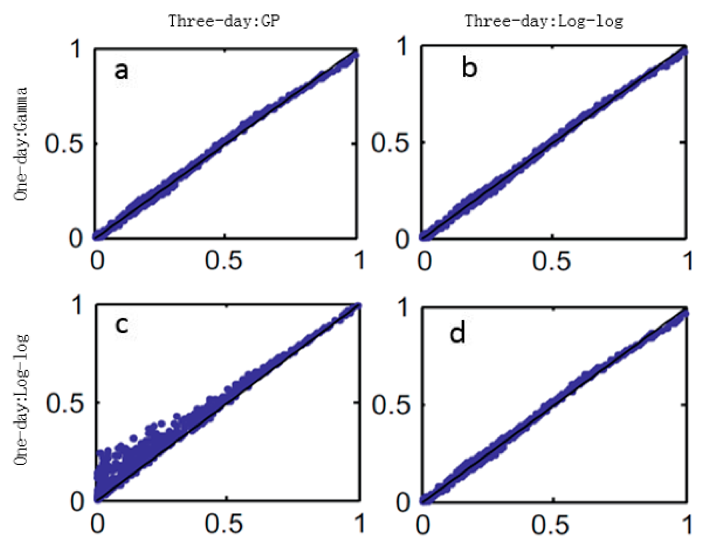
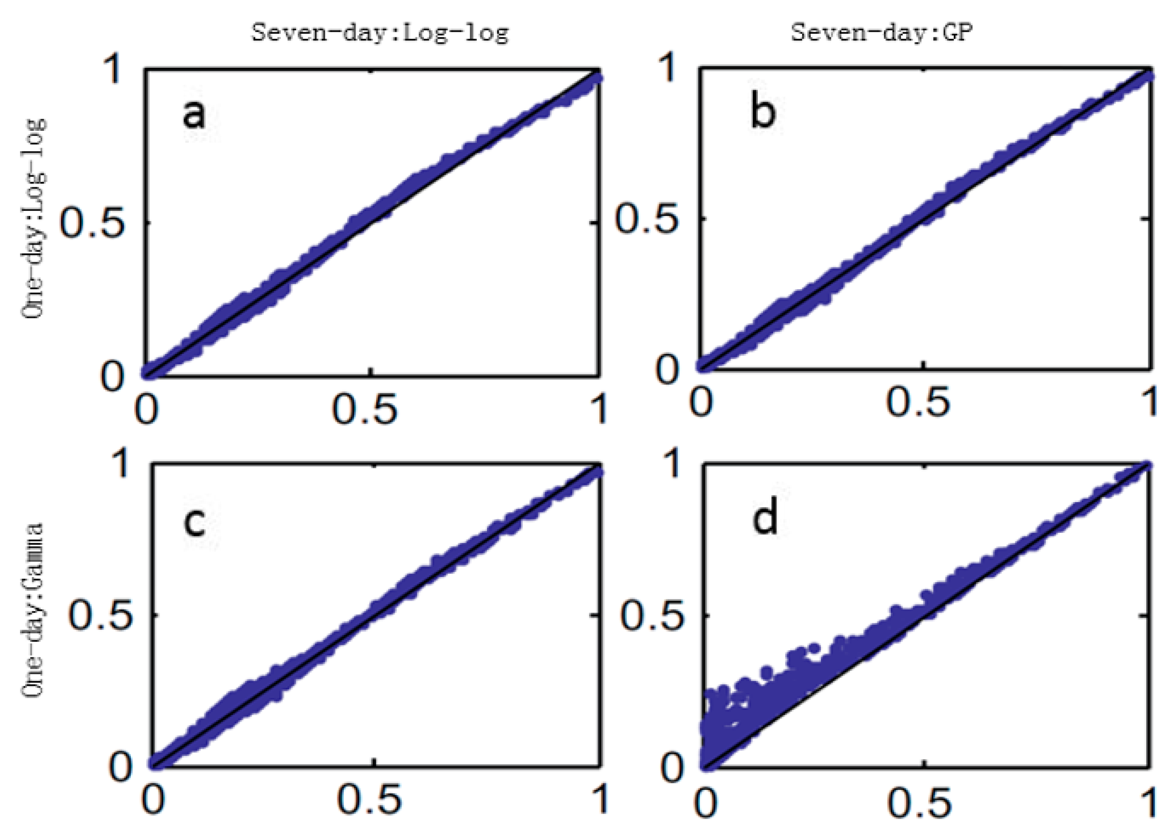
Figure 3 and Figure 4 show the Q-Q plots for the Gumbel and empirical copulas for different marginal distribution combinations. The cumulative probability of the empirical copula is represented by x-axis, and the y-axis represents the values of the Gumbel copula. The diagonal straight line represents a perfect match between the parametrically estimated copula and the empirical copula. Generally, the Q-Q plots confirm the results revealed from the statistical values in Table 6 and Table 7. That is, for one-day and three-day rainfall, the Gamma vs. GP pairs provide the best copula fitting results, which are chosen as the base case to compare the impact of marginal distributions and copulas whereas the Log–log vs. GEV pair is chosen as the base case to compare the impacts of the marginal distributions and copulas, but Log-log vs. GP is the worst pair. For one-day and seven-day rainfall, the Gamma vs. GP pairs provide the worst copula fitting results, whereas the Log–log vs. GP pair proved to be better.
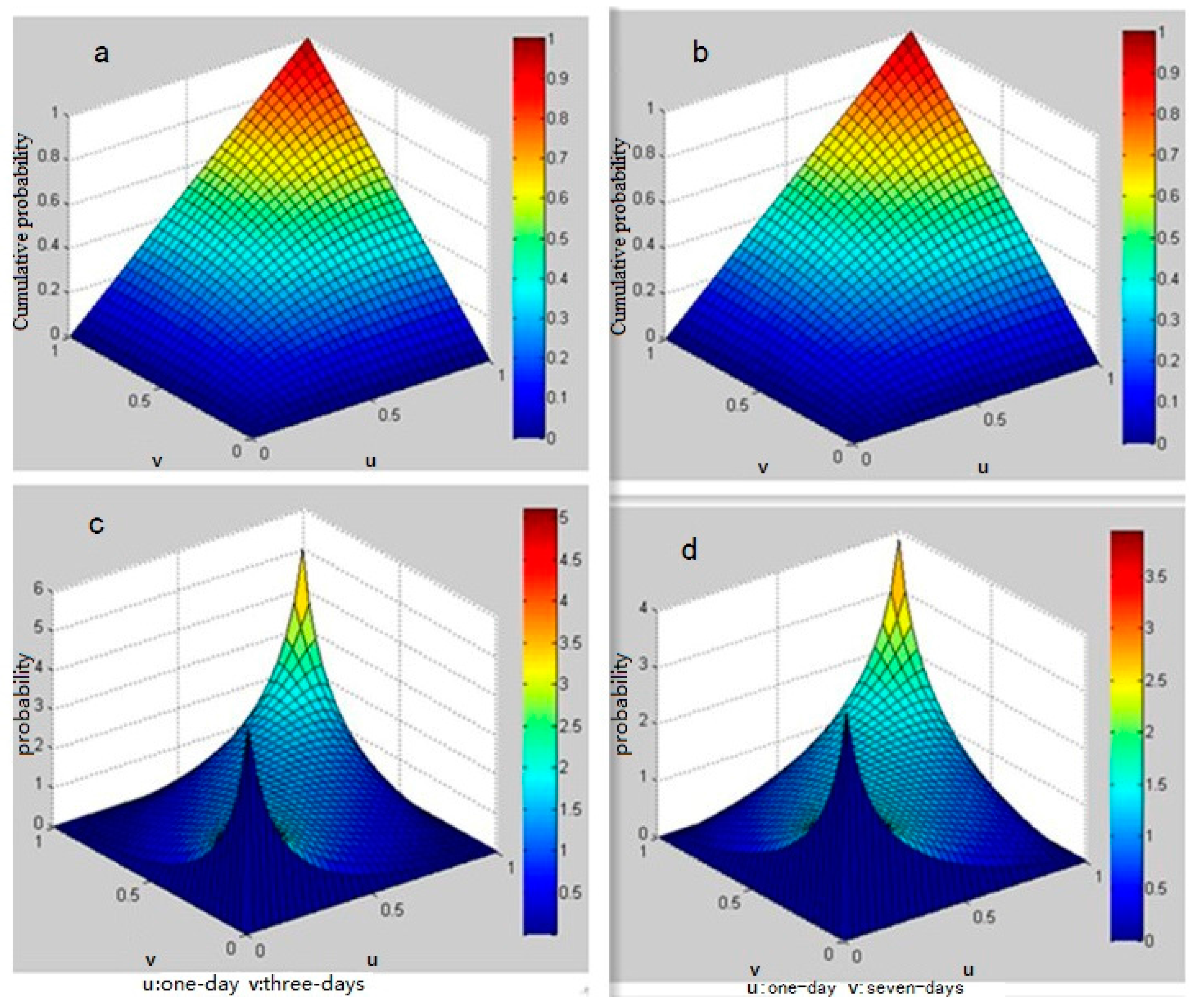
To understand the structure of dependence, Figure 5 visualises the cumulative distribution and probability distribution function of the Gumbel copula on the basis of the Gamma vs. GP and Log-log vs. GP combination for the two series. The variables u and v represent the transformed random variables X and Y in the unit hypercube, respectively, and have the same ranks as X and Y. Figure 4a,b show the fitted copula using a shaded surface. The strong dependence in the upper tail is clearly illustrated in Figure 4c,d.
Upper tail dependence is also important when considering copula. Table 8 shows the coefficients for Gumbel copulas of the series of one-day rainfall and three-day rainfall. As can be seen from the table, the estimated coefficient values are very close to the theoretical ones. More importantly, this implies that the choice of marginal distribution has little influence on tail dependence, which is mainly controlled by copulas as expected.
Selecting the suitable copula and its marginal distribution is a complex process that needs to consider all parts including statistics, graphical approaches, tail dependence analysis and comparison to empirical copulas. Incomplete research of copulas may fail to identify the inappropriate copulas and their marginal distribution, leading to an overestimate or underestimate of probability.

3.4. Conditional Probability

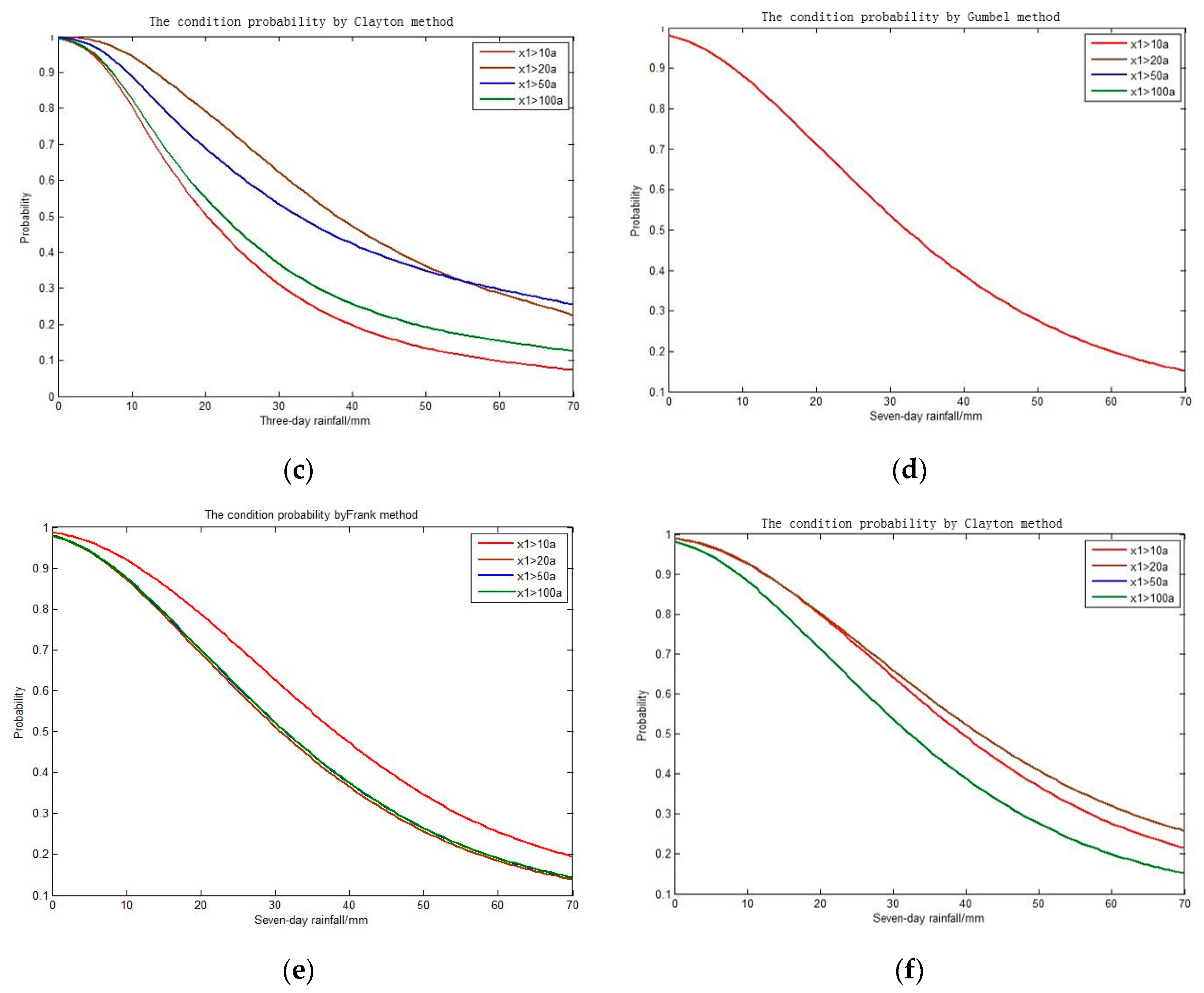
To reflect the connection between the one-day and multi-day rainfall, the conditional probability of multi-day rainfall can be calculated based on the reappearing period of one-day rainfall, and different copulas are used here to see the difference between them. Figure 6 shows the conditional probability of three-day and seven-day rainfall, which is when a one-day rainfall occurs over an x-year return period, the probability of three-day rainfall and seven-day rainfall occurs. For the series of one-day and three-day, Gamma vs. GP pairs are used, and for one-day and seven-day, Log-log vs. GP are used. Figure 6a–c show that when the one-day rainfall is over a value, the probability of three-day rainfall increases with the decrease in the value of precipitation, the conclusion is also correct with respect to seven-day rainfall. When the precipitation of a three-day rainfall is fixed, its probability increases with the same tendency as that of the precipitation of one-day rainfall. However, for fixed precipitation of one-day rainfall, the probability of seven-day rainfall changes according to the crosscurrent of the precipitation. However, the seven-day rainfall changes little compared to the three-day rainfall when the one-day rainfall changes.
In fact, from Figure 6 we can also see that for different conditional probabilities, the result of Gumbel is stable, which is in step with the results in Table 6 and Table 7. However, the curve of Clayton is unsteady, as the non-parametric estimate of the Clayton copula is significantly larger and is outside the 95% confidence interval. Note that according to the copula fitting results, the Clayton copula is not appropriate to describe the dependence structure, because the Clayton copula places more attention on the lower tail while the rainfall data shown in Figure 2 illustrate greater dependence on the upper tail than the lower tail. However, it is used here to demonstrate its potential impacts.

3.5. Impacts of Copulas and Marginal Distributions

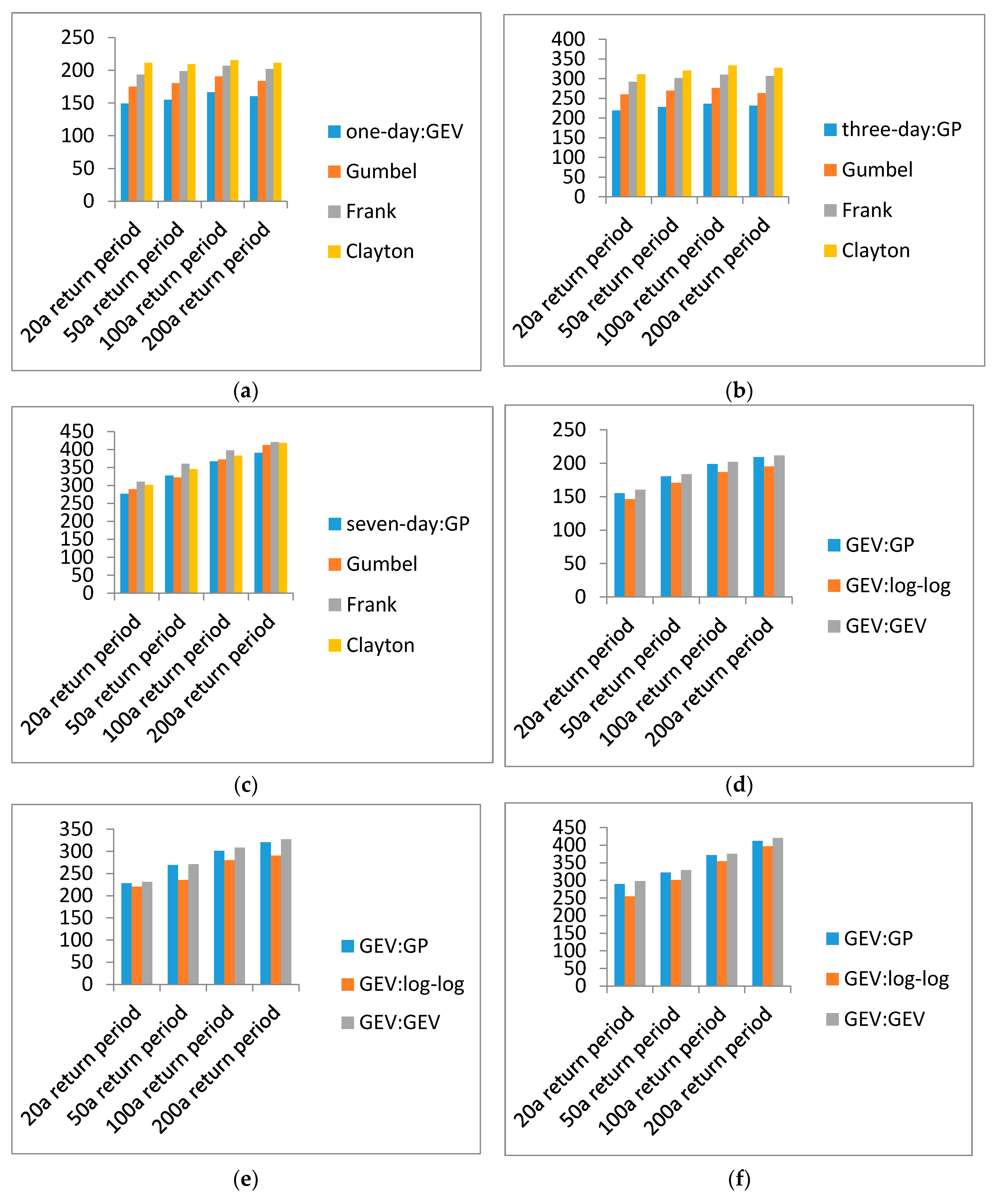
Different marginal distributions for one-day rainfall and multi-day rainfall cannot be rejected based on the statistical tests in this study. To investigate the impact of different marginal distributions, the joint return period was used to calculate the value of the different probabilities. Figure 7d–f show the value using the. Figure 7d–e were calculated using the one-day and three-day series, and Figure 7f was calculated using the one-day and seven-day series. For all marginal distribution combinations, the Gumbel copula is used to simulate the dependence structure between one-day rainfall and multi-day rainfall. For one-day, three-day and seven-day rainfall, the values of different pairs are roughly the same. The difference between different combinations of marginal distributions of the seven-day events is the greatest, while thosse of one-day events are small. This implies that the impacts of the different marginal distributions are negligible compared to the other uncertainties, such as copula parameter estimation, and the impact may decrease from seven-day rainfall to one-day rainfall.
Different copulas also reflect the value of one-day rainfall and multi-day rainfall. Here, marginal distributions are shown as contrast. For one-day, three-day and seven-day events, GEV, GP and GP are selected as marginal distributions. Gamma vs. GP pairs are used for the one-day and three-day series to calculate the value of one-day rainfall and three-day rainfall, while for one-day and seven-day, Log-log vs. GP are used to calculate the value of seven-day rainfall. The Gumbel copula is smaller than the Clayton and Frank copulas, and the Clayton value is considerably higher than that of marginal distributions. Similar to the results presented above, the Clayton copula was not appropriate to describe the structure of one-day rainfall and multi-day rainfall, which overestimates the value of different probabilities. Clearly, the copulas have a more significant impact than the marginal distributions. This implies the importance of considering the dependence structure of the one-day and multi-day rainfall when evaluating the system performance of a city’s flood control systems via copula methods.

4. Conclusions

This paper highlights the importance of considering the dependence structure of one-day and multi-day rainfall using copulas. The multi-day rainfall characteristics in the case study are represented by two cases: three-day and seven-day rainfall. The marginal distributions of these variables are simulated using GP, GEV, Log–log and Gamma, and the dependence structure is represented by the following three one-parameter Archimedean copula families: Gumbel, Frank, and Clayton. This methodology is promising in that it provides a simpler way to construct the joint distribution for rainfall events by separating the dependence from its marginal distributions. The conclusions determined from this study are as follows:
(1)
It is necessary to consider different marginal distributions that cannot be rejected by statistical tests for copula fitting rather than choosing the best ranked distributions. As revealed using bivariate copulas, the pair of the best fitted marginal distributions for the one-day and multi-day rainfall cannot produce the best overall performance during construction of the joint distribution of one-day and multi-day events.
(2)
Several different measures should be used to consider the best fit copula identification, including statistics, graphical approaches, tail dependence analysis and comparison to empirical copulas. Different measures can reflect different characteristics of copulas. A single measure may identify inappropriate copulas, leading to an overestimate or underestimate of the probability of a flood.
(3)
The copula method has flexibility and provides notable advantages in constructing complex, bivariate probability distributions for one-day and multi-day rainfall for system performance analysis. The results provide a more accurate probabilistic evaluation of precipitation for flood control based on the characterisation of the dependence structure for one-day and multi-day rainfall.
(4)
The designed maximum one-day precipitation and maximum three-day precipitation are important when we think about a city’s flood control system. However, it is meaningful to take the probabilistic relationships between the first day rainfall and the overall rainfall using multivariable joint distribution into account. This provides crucial information for more accurate estimation of storm designs and the associated risks.

Acknowledgments

This study was supported by the National Natural Science Foundation of China (Grant No. 51409270), the National Key Research and Development Program (Grant No. 2016YFA0601500), the International Science and Technology Cooperation Program of China (Grant No. 2013DFG70990), and the Foundation of China Institute of Water Resources and Hydropower Research (1232).

Author Contributions

All the authors contributed to the conception and development of this manuscript. Yang Wang carried out the analysis and wrote the paper. Chuanzhe Li reviewed and edited the manuscript. Jia Liu and Fuliang Yu conceived and designed the framework. Qingtai Qiu, Jiyang Tian and Mengjie Zhang provided assistance in calculations and figure productions.

Conflicts of Interest

The authors declare no conflict of interest.

References

  1. Liu, P.; Li, L.; Guo, S.; Xiong, L.; Zhang, W.; Zhang, J.; Xu, C.Y. Optimal design of seasonal flood limited water levels and its application for the Three Gorges Reservoir. J. Hydrol. 2015, 527, 1045–1053. [Google Scholar] [CrossRef]
  2. Seo, B.C.; Krajewski, W.F. Correcting temporal sampling error in radar-rainfall: Effect of advection parameters and rain storm characteristics on the correction accuracy. J. Hydrol. 2015, 531, 272–283. [Google Scholar] [CrossRef]
  3. Huang, S.; Hou, B.; Chang, J.; Huang, Q.; Chen, Y. Copulas-based probabilistic characterization of the combination of dry and wet conditions in the Guanzhong Plain, China. J. Hydrol. 2014, 519, 3204–3213. [Google Scholar] [CrossRef]
  4. Balistrocchi, M.; Grossi, G.; Bacchi, B. Deriving a practical analytical-probabilistic method to size flood routing reservoirs. Adv. Water Resour. 2013, 62, 37–46. [Google Scholar] [CrossRef]
  5. Molina, J.L.; Zazo, S.; Rodríguez-Gonzálvez, P.; González-Aguilera, D. Innovative Analysis of Runoff Temporal Behavior through Bayesian Networks. Water 2016, 8, 35–56. [Google Scholar] [CrossRef]
  6. Thorndahl, S.; Willems, P. Probabilistic modelling of overflow, surcharge and flooding in urban drainage using the first-order reliability method and parameterization of local rain series. Water Res. 2008, 42, 455–466. [Google Scholar] [CrossRef] [PubMed]
  7. Stephenson, A.G.; Lehmann, E.A.; Phatak, A. A max-stable process model for rainfall extremes at different accumulation durations. Weather Clim. Extrem. 2016, 13, 44–53. [Google Scholar] [CrossRef]
  8. Van de Vyver, H. Bayesian estimation of rainfall intensity–duration–frequency relationships. J. Hydrol. 2015, 529, 1451–1463. [Google Scholar] [CrossRef]
  9. Ma, T.; Li, C.; Lu, Z.; Bao, Q. Rainfall intensity—Duration thresholds for the initiation of landslides in Zhejiang Province, China. Geomorphology 2015, 245, 193–206. [Google Scholar] [CrossRef]
  10. Huang, Y.F.; Mirzaei, M.; Amin, M.Z.M. Uncertainty Quantification in Rainfall Intensity Duration Frequency Curves Based on Historical Extreme Precipitation Quantiles. Procedia Eng. 2016, 154, 426–432. [Google Scholar] [CrossRef]
  11. Favre, A.C.; El Adlouni, S.; Perreault, L.; Thiémonge, N.; Bobée, B. Multivariate hydrological frequency analysis using copulas. Water Resour. Res. 2004, 40, 67–79. [Google Scholar] [CrossRef]
  12. Li, F.; Zheng, Q. Probabilistic modelling of flood events using the entropy copula. Probabilistic modelling of flood events using the entropy copula. Adv. Water Resour. 2016, 97, 233–240. [Google Scholar] [CrossRef]
  13. Durocher, M.; Chebana, F.; Ouarda, T.B. On the prediction of extreme flood quantiles at ungauged locations with spatial copula. J. Hydrol. 2015, 533, 523–532. [Google Scholar] [CrossRef]
  14. Fu, G.; Butler, D.; Khu, S.T. Multiple objective optimal control of integrated urban wastewater systems. Environ. Model. Softw. 2008, 23, 225–234. [Google Scholar] [CrossRef]
  15. Frahm, G.; Junker, M.; Schmidt, R. Estimating the tail dependence coefficient: Properties and pitfalls. Insur. Math. Econ. 2005, 37, 80–100. [Google Scholar] [CrossRef]
  16. Nazemi, A.; Elshorbagy, A. Application of copula modelling to the performance assessment of reconstructed watersheds. Stoch. Environ. Res. Risk Assess. 2012, 26, 189–205. [Google Scholar] [CrossRef]
  17. Targino, R.S.; Peters, G.W.; Shevchenko, P.V. Sequential Monte Carlo Samplers for capital allocation under copula-dependent risk models. Insur. Math. Econ. 2015, 61, 206–226. [Google Scholar] [CrossRef]
  18. Meintanis, S.G.; Ngatchou-Wandji, J.; Taufer, E. Goodness-of-fit tests for multivariate stable distributions based on the empirical characteristic function. J. Multivar. Anal. 2015, 140, 171–192. [Google Scholar] [CrossRef]
  19. Aghakouchak, A.; Ciach, G.; Habib, E. Estimation of tail dependence coefficient in rainfall accumulation fields. Adv. Water Res. 2010, 33, 1142–1149. [Google Scholar] [CrossRef]
  20. Fu, G.; Butler, D. Copula-based frequency analysis of overflow and flooding in urban drainage systems. J. Hydrol. 2014, 510, 49–58. [Google Scholar] [CrossRef] [Green Version]
  21. Ma, M.W.; Ren, L.L.; Song, S.B.; Song, J.L.; Jiang, S.H. Goodness-of-fit tests for multi-dimensional copulas: Expanding application to historical drought data. Water Sci. Eng. 2013, 6, 18–30. [Google Scholar]
  22. Villarini, G.; Serinaldi, F.; Krajewski, W.F. Modeling radar-rainfall estimation uncertainties using parametric and non-parametric approaches. Adv. Water Res. 2008, 31, 1674–1686. [Google Scholar] [CrossRef]
  23. Montes-Iturrizaga, R.; Heredia-Zavoni, E. Reliability analysis of mooring lines using copulas to model statistical dependence of environmental variables. Appl. Ocean Res. 2016, 59, 564–576. [Google Scholar] [CrossRef]
  24. Joe, H. Multivariate Models and Dependence Concepts; Chapman and Hall: London, UK, 1997. [Google Scholar]
  25. Bazargani, N.; Nosratinia, A. Joint maximum likelihood estimation of activation and Hemodynamic Response Function for FMRI. Med. Image Anal. 2014, 18, 711–724. [Google Scholar] [CrossRef] [PubMed]
  26. Kao, S.C.; Govindaraju, R.S. Probabilistic structure of storm surface runoff considering the dependence between average intensity and storm duration of rainfall events. Water Sci. Eng. 2007, 430, 491–496. [Google Scholar] [CrossRef]
  27. Genest, C.; Favre, A.C. Everything You Always Wanted to Know about Copula Modeling but Were Afraid to Ask. J. Hydrol. Eng. 2007, 12, 347–368. [Google Scholar] [CrossRef]
  28. Chatzithomas, C.D.; Alexandris, S.G. Solar radiation and relative humidity based, empirical method, to estimate hourly reference evapotranspiration. Agric. Water Manag. 2015, 152, 188–197. [Google Scholar] [CrossRef]
  29. Genest, C.; Rivest, L.P. Statistical Inference Procedures for Bivariate Archimedean Copulas. J. Am. Stat. Assoc. 1993, 88, 1034–1043. [Google Scholar] [CrossRef]
  30. Vandenberghe, S.; Verhoest, N.E.C.; De Baets, B. Fitting bivariate copulas to the dependence structure between storm characteristics: A detailed analysis based on 105 year 10 min rainfall. Water Resour. Res. 2010, 46, 489–496. [Google Scholar] [CrossRef]
  31. Basinger, M.; Montalto, F.; Lall, U. A rainwater harvesting system reliability model based on nonparametric stochastic rainfall generator. J. Hydrol. 2010, 392, 105–188. [Google Scholar] [CrossRef]
  32. Di Bernardino, E.; Rulliere, D. On tail dependence coefficients of transformed multivariate Archimedean copulas. Fuzzy Sets Syst. 2016, 284, 89–112. [Google Scholar] [CrossRef]
  33. Hua, L.; Joe, H. Strength of tail dependence based on conditional tail expectation. J. Multivar. Anal. 2014, 123, 143–159. [Google Scholar] [CrossRef]
  34. Keylock, C.J. Describing the recurrence interval of extreme floods using nonextensive thermodynamics and Tsallis statistics. Adv. Water Resour. 2005, 28, 773–778. [Google Scholar] [CrossRef]
  35. Zhang, J.; Lin, X.; Guo, B. Multivariate Copula-Based Joint Probability Distribution of Water Supply and Demand in Irrigation District. Water Resour. Manag. 2016, 30, 2361–2375. [Google Scholar] [CrossRef]
  36. Nelsen, R.B. An Introduction to Copulas; Springer: New York, NY, USA, 2006. [Google Scholar]
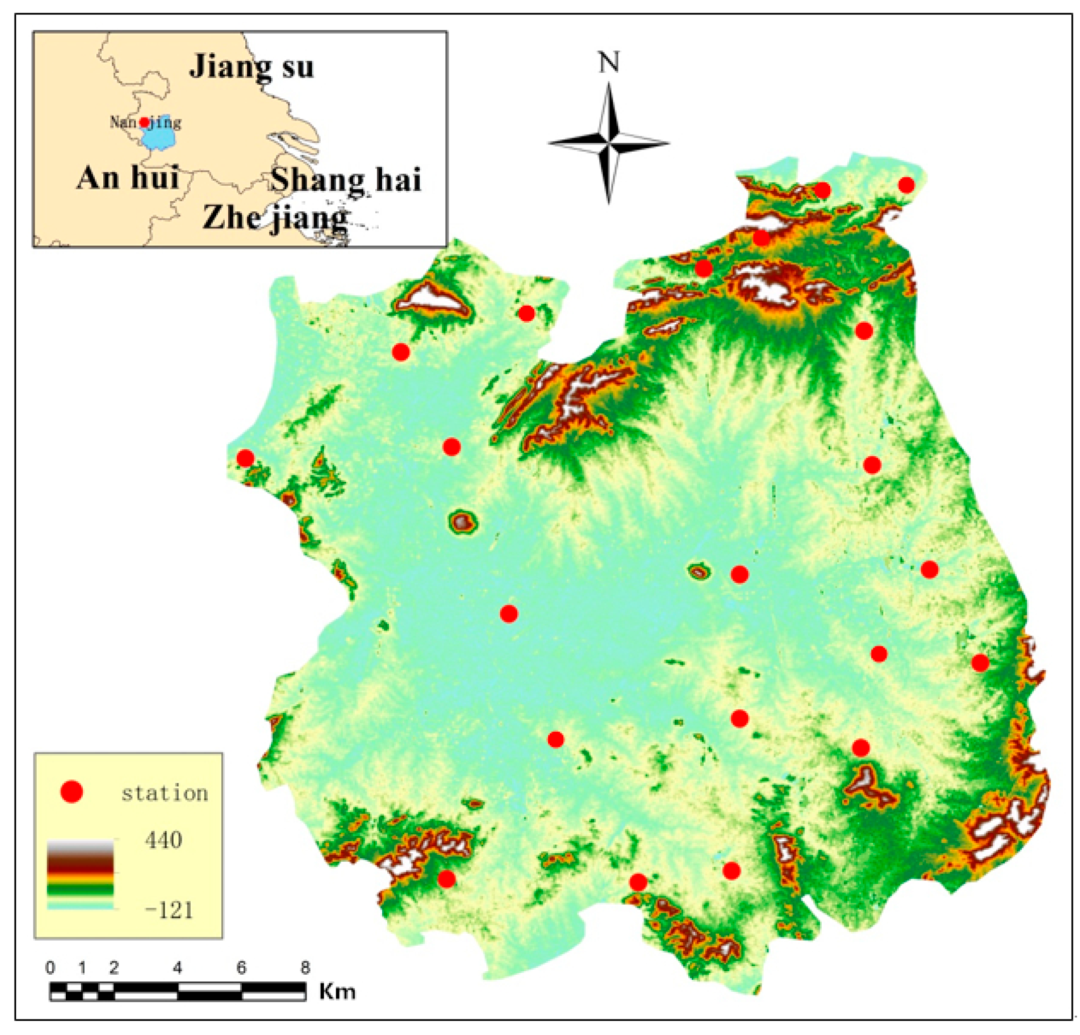
Figure 1. The location of the study area and the locations of the meteorological stations in the study area.
Water 09 00198 g001
Figure 2. Scatter plots of the one-day and multi-day rainfall with marginal histograms. (a) one-day and three-day rainfall (b) one-day and seven-day rainfall.
Water 09 00198 g002
Figure 3. Q-Q plots for the Gumbel and empirical copulas for different marginal distribution combinations of one-day rainfall and three-day rainfall. (a) Gamma (one-day) vs. GP (three-day); (b) Gamma (one-day) vs. Log-log (three-day); (c) Log-log(one-day) vs. GP (three-day); (d) Log-log (one-day) vs. Log-log (three-day).
Water 09 00198 g003
Figure 4. Q-Q plots for the Gumbel and empirical copulas for different marginal distribution combinations of one-day rainfall and seven-day rainfall. (a) Log-log (one-day) vs. Log-log (seven-day); (b) Log-log (one-day) vs. GP (seven-day); (c) Gamma (one-day) vs. Log-log (seven-day); (d) Gamma (one-day) vs. GP (seven-day).
Water 09 00198 g004
Figure 5. Three-dimensional plots for the theoretically fitted Gumbel copula. (a) fitted copula using a shaded surface of one-day and three-day; (b) fitted copula using a shaded surface of one-day and seven-day; (c) upper tail correlation of one-day and three-day; (d) upper tail correlation of one-day and seven-day.
Water 09 00198 g005
Figure 6. Frequency curves of the conditional probabilities. (a) one-day and three-day using Gumbel; (b) one-day and three-day using Frank; (c) one-day and three-day using Clayton; (d) one-day and seven-day using Gumbel; (e) one-day and seven-day using Frank; (f) one-day and seven-day using Clayton.
Water 09 00198 g006aWater 09 00198 g006b
Figure 7. Design values for a single variable and two-dimensional copula joint distributions. (a) GEV (one-day) vs. copulas (one-day); (b) GP (three-day) vs. copulas (three-day); (c) GP (seven-day) vs. copulas (seven-day); (d) one-day rainfall of Gumbel using different marginal distributions; (e) three-day rainfall of Gumbel using different marginal distributions; (f) seven-day rainfall of Gumbel using different marginal distributions.
Water 09 00198 g007
Table 1. Daily precipitation data series.
NO.Name of Rain StationDate Series
1qinhuai new river sluice1967–1968, 1981–1982, 1987–2010
2wudingmen sluice1961–2010
3tiansheng bridge sluice1953–2010
4qianhan village1965–1969, 1978–2010
5east mountain1953–2010
6jurong1953–2010
7zhaocun reservoir1955–1960, 1962–2010
8anjishan reservoir1953–1910
9linchang1965–2001
10tingzi1967–2001
11xixie1967–2001
12aiyuan1967–2001
13chishan new sluice1960–2010
14tianwangsi1953–1961, 1963–1999
15qilin1967–1968, 1978–1999
16north mountain reservoir1960–1988, 1991, 1996–2010
17ershengqiao reservoir1962–1988, 2000–2010
18maoshan reservoir1978–1988, 2004–2010
19fangbian reservoir1954, 1957, 1958, 1960–1966, 1991, 1996–2010
20wolongshan reservoir2004–2010
21zhongshan reservoir1977–1979, 2004–2010
Table 2. Test statistics for the fitted cumulative distribution for one-day and three-day rainfall.
Date SeriesDistributionK–Sp-Value
Kn
one-day rainfallGEV0.0170.833
Gamma0.0230.510
Log-Log0.0360.429
GP0.0490.065
three-day rainfallGP0.0190.910
Log-Log0.0250.176
GEV0.0380.091
Gamma0.0420.091
Table 3. Test statistics for the fitted cumulative distribution for one-day and seven-day rainfall.
Date SeriesDistributionK–Sp-Value
Kn
one-day rainfallGEV0.0220.072
Log-Log0.0320.047
Gamma0.0430.037
GP0.0540.006
seven-day rainfallGP0.0191.003
Log-Log0.0310.194
GEV0.0480.103
Gamma0.0560.111
Table 4. Parameters for the copulas and their 95% confidence intervals for one-day and three-day rainfall.
One-Day RainfallThree-Day RainfallGumbelConfidence IntervalFrankConfidence IntervalClaytonConfidence Interval
GEVGP1.375[1.285, 1.466]2.472[1.971, 2.974]0.443[0.317, 0.570]
Log-Log1.399[1.309, 1.489]2.412[1.916, 2.909]0.393[0.273, 0.513]
GEV1.372[1.280, 1.465]2.546[2.032, 3.059]0.413[0.288, 0.539]
GammaGP1.377[1.280, 1.465]2.509[1.997, 3.021]0.375[0.257, 0.494]
Log-Log1.403[1.284, 1.470]2.447[1.940, 2.953]0.340[0.227, 0.453]
GEV1.375[1.311, 1.496]2.591[2.067, 3.114]0.354[0.237, 0.471]
Log-LogGP1.382[1.281, 1.470]2.845[2.290, 3.400]0.507[0.344, 0.671]
Log-Log1.403[1.288, 1.476]2.447[1.940, 2.953]0.340[0.227, 0.453]
GEV1.385[1.311, 1.496]3.063[2.502, 3.623]0.473[0.323, 0.623]
Table 5. Parameters for the copulas and their 95% confidence intervals for one-day and seven-day rainfall.
One-Day RainfallSeven-Day RainfallGumbelConfidence IntervalFrankConfidence IntervalClaytonConfidence Interval
GEVGP1.100[1.028, 1.173]2.101[1.964, 2.240]0.399[0.373, 0.425]
Log-Log1.119[1.046, 1.193]2.050[1.916, 2.186]0.354[0.331, 0.377]
GEV1.098[1.026, 1.170]2.164[2.032, 2.307]0.372[0.347, 0.396]
Log-LogGP1.102[1.029, 1.175]2.133[1.993, 2.274]0.338[0.315, 0.360]
Log-Log1.122[1.049, 1.197]2.080[1.944, 2.218]0.306[0.286, 0.326]
GEV1.100[1.028, 1.173]2.202[2.058, 2.348]0.319[0.298, 0.340]
GammaGP1.106[1.033, 1.179]2.418[2.260, 2.578]0.456[0.426, 0.486]
Log-Log1.122[1.049, 1.197]2.080[1.944, 2.218]0.306[0.286, 0.326]
GEV1.108[1.035, 1.181]2.604[2.433, 2.776]0.426[0.398, 0.454]
Table 6. Goodness-of-fit of the copulas for different combinations of marginal distributions of one-day and three-day rainfall.
One-Day RainfallThree-Day RainfallGumbelFrankClayton
RMSETnRMSETnRMSETn
GEVGP0.0140.1110.0150.1190.0130.102
Log-Log0.0160.1470.0160.1400.0130.099
GEV0.0150.1380.0200.2120.0160.166
GammaGP0.0110.0620.0140.1030.0160.168
Log-Log0.0130.0910.0150.1270.0170.169
GEV0.0140.1020.0190.2080.0200.242
Log-LogGP0.0612.0780.0743.0410.0481.421
Log-Log0.0130.0910.0150.1270.0170.169
GEV0.0592.0170.0793.4810.0481.458
Table 7. Goodness-of-fit of the copulas for different combinations of marginal distributions of one-day and seven-day rainfall.
One-Day RainfallSeven-Day RainfallGumbelFrankClayton
RMSETnRMSETnRMSETn
GEVGP0.0130.1110.0120.1240.0110.102
Log-Log0.0140.1470.0130.1210.0110.099
GEV0.0140.1380.0160.2010.0140.166
Log-LogGP0.0100.0620.0110.2040.0140.168
Log-Log0.0110.0910.0120.2050.0150.169
GEV0.0120.1020.0150.2930.0180.242
GammaGP0.0521.9180.0601.7260.0421.421
Log-Log0.0110.0910.0120.2050.0150.169
GEV0.0532.0170.0641.7710.0421.458
Table 8. The upper tail dependence coefficients for Gumbel copulas.
One-DayGEVGammaLog-Log
Three-dayGPLog-LogGEVGPLog-LogGEVGPLog-LogGEV
ƛu0.3370.3520.3360.3390.3540.3370.3420.3540.344
ƛ ^ u0.3440.3630.3450.3490.3610.3460.3470.3600.350