Article

Projection of Climate Change Scenarios in Different Temperature Zones in the Eastern Monsoon Region, China

1
Beijing Key Laboratory of Urban Hydrological Cycle and Sponge City Technology, College of Water Sciences, Beijing Normal University, Beijing 100875, China
2
Institute of Tibetan Plateau Research, Chinese Academy of Science, Beijing 100101, China
*
Author to whom correspondence should be addressed.
Water 2017, 9(5), 305; https://doi.org/10.3390/w9050305
Submission received: 9 February 2017 / Revised: 24 April 2017 / Accepted: 25 April 2017 / Published: 27 April 2017

Abstract

:
The Eastern Monsoon Region of China is sensitive to climate change because of its special location. In this study, the Automated Statistical Downscaling (ASD) tool was used to simulate and project future climate change scenarios in different temperate zones in the Eastern Monsoon Region of China. The performances of the single General Circulation Model (GCM) and the GCMs ensemble from Coupled Model Inter-comparison Project Phase 5 (CMIP5) were compared, and the capability of the ASD model was evaluated. The simple mathematical averaging ensemble of GCMs is superior to the single GCM and to the other two weighted ensembles. The ASD model was capable of presenting the temporal and spatial variation of four variables (precipitation, mean air temperature, maximum and minimum air temperature) during both the calibration and validation periods. The performance of the ASD model varied among the different temperate zones. In the simulated future scenarios, the air temperature in the four zones showed an upward trend. Except for the subtropical zone, there was a tendency for increased precipitation in both the warm temperate zone and the cold temperate and middle temperate zones. Of particular interest is that, in the subtropical zone, the precipitation will decline in the future, whereas the air temperature (especially the maximum air temperature) will increase, which may put more pressure on water resource situations in this area.

1. Introduction

According to the fifth assessment report by the Intergovernmental Panel on Climate Change (IPCC), there is no doubt that the temperature has increased during the past century. From 1880 to 2012, the global surface air temperature has increased by 0.85 °C. The warming trends will continue in this century, with an increase of 0.3–4.8 °C expected by the end of the century [1]. Global warming will have a significant impact on local climatic and hydrologic processes, resulting in a series of problems such as mutated water cycles, inhomogeneous spatial distribution of precipitation, and more frequent extreme climatic and hydroligical events, which in turn will affect the ecological, social, and economic systems of human society. Therefore, it is essential to perform qualitative and quantitative predictions of future climate change scenarios from a regional perspective.
The General Circulation Models (GCMs) are often employed to simulate global and regional climate systems. However, such models can only provide information at a coarse resolution [2,3], which cannot be used directly in regional hydrological modelling [4,5]. However, this deficiency can be compensated for by the application of downscaling techniques [6]. On the basis of large-scale GCMs output, climate scenarios with finer resolution can be achieved using downscaling methods. Considering that the hydrologic impacts of climate change vary from region to region [7,8,9], finer resolution scenarios can be employed as an input in hydrology; for instance, in runoff simulation. Downscaling methods fall into two general categories; dynamical downscaling and statistical downscaling [10,11,12,13,14]. Until now, the most common dynamic approach has been to run a regional climate model at high resolution nested within a GCM at coarse resolution. Despite its drawbacks such as the requisition of high computer configuration, the heavy computational burden, and the need for professional meteorological background knowledge [15], this approach has been widely implemented [16,17,18].
The basis of statistical downscaling methods is the establishment of statistical relationships with clear physical meanings between large scale climate predictors and fine resolution ground observations [19]. The method is capable of correcting systematic errors in GCMs’ output with less computational complexity and a higher feasibility [20]. There are several statistical downscaling methods, and the availability of these methods varies between different regions [21,22,23,24,25].
Climate change has become a significant issue. A number of studies on the topic of statistical downscaling methods have been conducted in China [26,27,28,29,30]. Most of the previous researches focused on particular regions or basins. However, no comprehensive study at the regional or mega scale under heterogeneous heat conditions has been conducted. The Eastern Monsoon Region, covering eight river basins and five temperate zones, has a monsoonal climate, which significantly affected social-economic development in the region. Good knowledge of future climate change scenarios will be of great significance in assessing the risk of droughts and floods in the future, and these results could further be utilized for planning the sustainable utilization of water resources in the region.
In this study, the ASD (Automated Statistical Downscaling) was adopted to investigate the future climate scenarios in five temperate zones in the Eastern Monsoon Region, and the evaluation of the performance of the ASD in these temperate zones of the Eastern Monsoon Region was performed. The objectives of this study were to: (1) compare the performance of the single GCM and the GCMs ensemble in order to prepare the data required for input into the ASD model; (2) evaluate the capability of the ASD model to reveal the temporal and spatial characteristics of precipitation and air temperature; and (3) generate future climate change scenarios in five temperate zones in the Eastern Monsoon Region of China. The results from the study provide a valuable database for future climate change scenarios in the Eastern Monsoon Region.

2. Study Area and Data Description
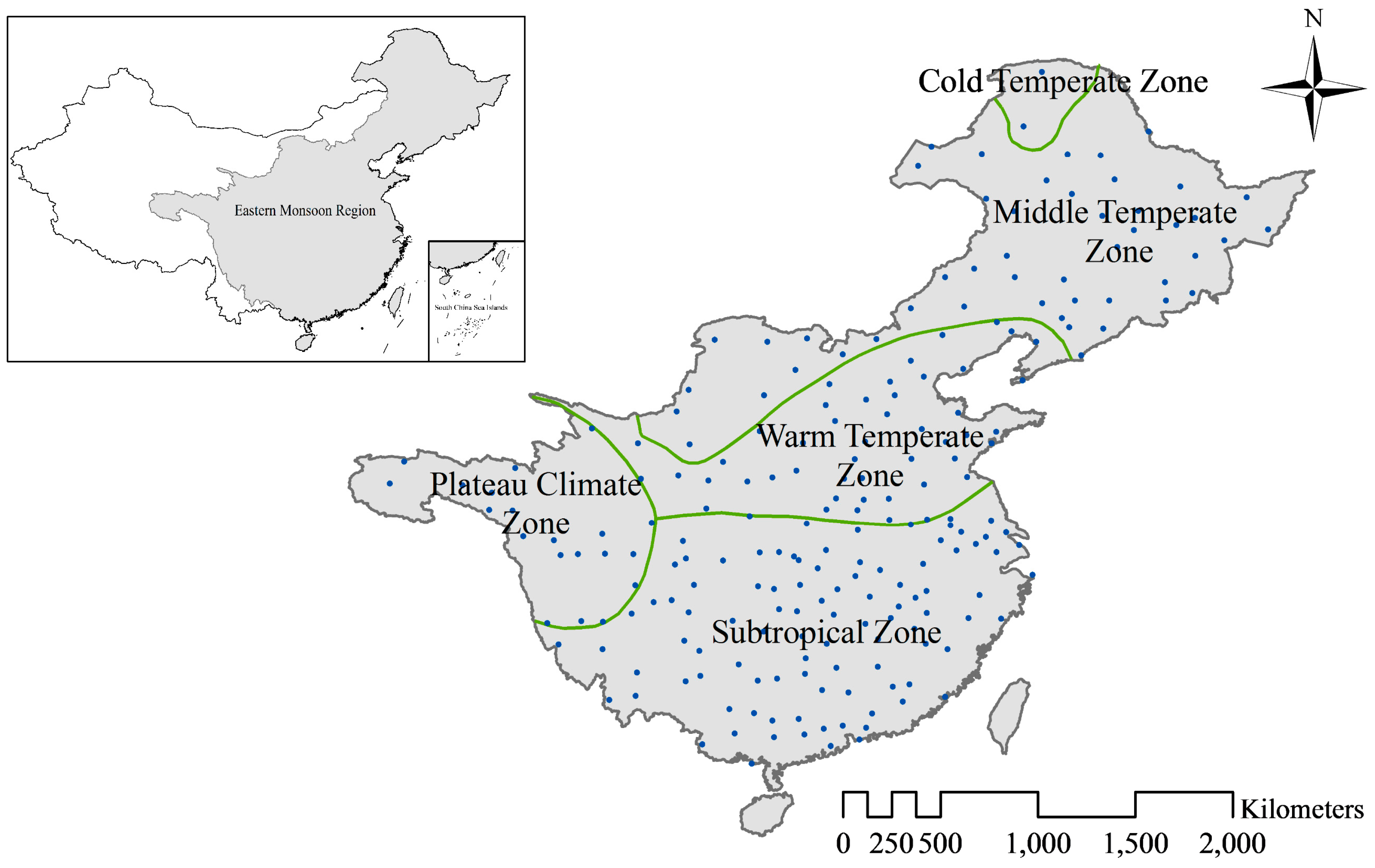
2.1. Study Area

The Eastern Monsoon Region is the most developed region in China, accounting for 46% of China’s land and 95% of its population. The region is sensitive to climate change, with severe water issues. It is considered a core area in water resources planning at the national level.
To reflect the heat distribution conditions in the different regions, the whole area of China was divided into six temperate zones based on the cumulative temperature. This method was adopted in our study to explore future climate change scenarios in different temperate zones. The Eastern Monsoon Region covers five temperate zones; the cold temperate zone (CTZ), middle temperate zone (MTZ), warm temperate zone (WTZ), subtropical zone (STZ), and the plateau climate zone (PCZ), as shown in Figure 1. There are only two meteorological stations in the cold temperate zone that can provide integral long time serial data. In addition, the cold temperate zone and middle temperate zone have similar climatic conditions. Therefore, the two zones were combined together in this research, abbreviated as the CMT Zone.

2.2. Data Description

To build and validate the statistical downscaling model, a large set of data is required for both predictors and predictands.
The observed daily data from 1961 to 2010 collected at 209 national meteorological observatory stations (Figure 1) were used in this research, including daily precipitation, mean air temperature, and maximum and minimum air temperature. The locations of the gauging stations can be seen in Figure 1. The stations covering the entire research area are uniformly distributed.
The reanalysis dataset is from the European Centre for Medium-Range Weather Forecasts (hereafter named ERA-40), ranging from 1957 to 2002 with a spatial resolution of 2.5° (long.) × 2.5° (lat.). Eleven ERA-40 variables are used as the predictors in our study, including 500 hPa specific humidity, 850 hPa specific humidity, sea-level pressure, 500 hPa air temperature, 850 hPa air temperature, surface air temperature, 850 hPa zonal wind, surface zonal wind, 500 hPa geopotential height, 700 hPa geopotential height, and 850 hPa geopotential height. The data from 1961 to 1990 was adopted as observed in large-scale climate fields. During calibration, statistical relationships between local observed meteorological variables (the ‘predictands’) and observed large-scale climate fields (the “predictors”) were developed.
Based on CMIP5, a total of 19 GCMs under scenario RCP4.5 (medium greenhouse gas emission scenario), derived by different institutions, were used in this research. The dataset was obtained from the Data Distribution Centre (DDC) of the Intergovernmental Panel on Climate Change (IPCC). The detailed information of the 19 GCMs is listed in Table 1.

3. Methodology

3.1. Assessment on GCMs Performance

As the 19 GCMs models perform differently, it is necessary to first evaluate the simulation efficiency. Different methods of doing this have been demonstrated in the literature on GCM evaluations [3,31]. The method of Rank Score was adopted in this research, using a group of statistics, which includes VC (Variation Coefficient), RMSE (Root Mean Squared Error), SPCC (Spatial Pearson Correlation Coefficient), TPCC (Temporal Pearson Correlation Coefficient), and LT (Linear Trend) as objective functions, and given different weighting values between 0 and 9. Rank Score is capable of assessing mean value, standard deviation, spatial and temporal distribution, and variation trends comprehensively. A smaller Rank Score would indicate a better GCM. The formula of the Rank Score is expressed as:
R S i = { I n t [ x i x min x max x min × 10 ] , x i < x max      9           , x i = x max
where xi is the relative error of the GCM simulation deviate from the observation, i is the number of GCMs adopted in the research, and xmin and xmax are the minimum and maximum values of the relative error, respectively. The function “Int” truncates a number to yield the integer portion of the number. A smaller xi results in a smaller RSi.
The performance comparison between a single GCM and the GCM ensemble was also undertaken, which aims to search for preferable GCM data. The GCM ensemble data were derived in two ways; by computing the simple mathematical average of the 19 models and through a weighted average method, in which the weight values were determined according to the two skill scores, S1 and S2 in Taylor’s study [32]. The formulas for the skill scores are as follows:
S 1 = 4 ( 1 + R ) ( σ + 1 σ ) 2 ( 1 + R 0 )
S 2 = 4 ( 1 + R ) 4 ( σ + 1 σ ) 2 ( 1 + R 0 ) 4
σ = S D g c m S D o b s
where R is the correlation coefficient between the GCM simulations and observations, R0 is the maximum value of R, and SDgcm and SDobs are the standard deviations of the GCM simulation and observation, respectively. When SDgcm and R are close to SDobs and R0, respectively, the skill scores will be close to 1, which indicates better performance of the model. Conversely, if the ratio of SDgcm to SDobs is close to 0 or infinity or if R is close to −1, the skill scores will approach 0, indicating a lower simulation capability of the model. The function of the standard deviation is emphasized in S1, whereas S2 lays more stress on the correlation coefficient between the simulation and observation.

3.2. ASD (Automated Statistical Downscaling) Model

The regression-based ASD model was inspired by the SDSM (Statistical Downscaling Model) and was developed by Hessami [33] using Matlab. Considering that air temperature is directly influenced by large scale predictors, modeling of the temperature event in ASD is unconditional and is performed in one step:
T i = γ 0 + j = 1 n γ j p i j + e i
where Ti is the temperature, n is number of predictors, pij is the predictor, and γ is the model parameter. The residual term ei is modeled as a Gaussian distribution:
e i = V I F / 12 z i S e + b
where zi is a normally distributed random number, Se is the standard error of the estimate, VIF is the variance inflation factor, and b is the model bias, which can be set using the following equations:
b = M o b s M d
V I F = 12 ( V o b s V d ) / S e 2
where Mobs and Md are the mean of the observations and the mean of the deterministic part of the model output during the calibration period, Vobs is the variance of the observations during the calibration period, Vd is the variance of the deterministic part of the model output during the calibration period, and Se is the standard error.
Modeling of a precipitation event is conditional because the occurrence of precipitation events must be determined first:
O i = α 0 + j = 1 n α j p i j
where Oi is the daily precipitation occurrence and α is a model parameter.
Two regression methods were used in the ASD model to build a statistical relationship between large scale predictors and regional predictands. Linear regression and ridge regression are used when strong correlation between the predictors is exhibited. Unlike the case in SDSM in which the selection of predictors is an iterative process and partly relies on a user’s subjective regression [34], the ASD model predictor selection process involves predictors being selected using a backward stepwise regression method. Furthermore, ASD is user friendly and is suitable for processing batch data.

4. Results and Discussion

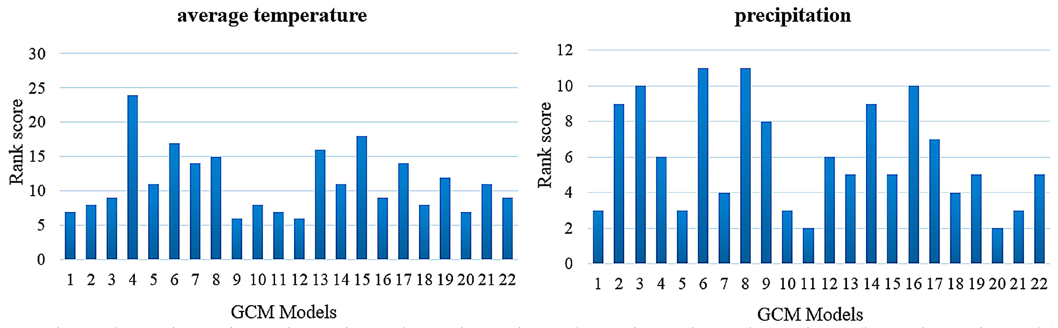
4.1. Assessment of GCMs Performance

The rank scores of the different GCMs and the GCMs ensembles determined are shown in Figure 2. The number ranging from 1 to 19 on the X-axis stands for the different GCMs listed in Table 1; number 20 represents the GCMs ensemble using a simple mathematical average method; and numbers 21 and 22 represent the weighted GCMs ensembles based on the skill scores S1 and S2. From the results, the GCMs ensembles are consistently superior to single models, and the simple averaging ensemble is superior to the weighted averaging ensembles. Hence, the simple averaging GCMs ensemble (MGCM) was adopted in the following research to provide future climate scenarios with high resolution.

4.2. Selection of Predictors

Statistical downscaling is based on the fundamental assumption that climate is conditioned by local physiographic characteristics as well as the larger scale atmospheric state. Based on this assumption, statistical relationships between local observed meteorological variables (the “predictands”) and observed global scale fields from ERA-40 reanalysis data (“the predictors”) may be developed. To identify the statistical relationships between large scale predictors and local predictands, it is important to first select global scale circulation factors that predict regional climatic variables. In the ASD model, the first step is to choose the proper predictors. In this study, all predictors are from ERA-40 reanalysis data, and all predictands are from in-situ observational data. The ASD method involves building a regression model between each predictand and all predictors. Once the explained variance exceeds 90% or higher, the predictors included in the regression model are reliable predictors and then are chosen for the next projection. Following the rules of predictor selection in statistical downscaling, eleven general circulation factors from the ERA-40 reanalysis data, which possess high correlation with local variables in the research area, were adopted as candidate predictors, including hus500 (500 hPa humidity field), hus850 (850 hPa humidity field), slp (sea-level pressure), ta500 (500 hPa temperature field), ta850 (850 hPa temperature field), tas (surface air temperature), ua850 (850 hPa zonal wind), uas (surface zonal wind), zg500 (500 hPa geopotential height field), zg700 (700 hPa geopotential height field), and zg850 (850 hPa geopotential height field). In the process of calibration, either four or five of these eleven candidate predictors were screened to establish correlation with local predictands.
The Eastern Monsoon Region is subject to the East Asian Monsoon, for which the dominant atmospheric circulation systems change dramatically in different seasons, influencing the selection of predictors. As shown in Figure 3, different local variables such as precipitation and air temperature are influenced by different atmospheric predictors. For the air temperature, tas and uas are the dominant factors; for precipitation, ta500 and ua850 play more important roles and the influence of uas is negligible. From a spatial perspective, the selected predictors vary from zone to zone. In the CMZ, WTZ, and STZ, tas is of relative higher significance among the predictors, whereas in the PCZ, the influence of tas is weak and the major factors are ta500 and hus500, which may be related to the more complicated geological and climatic conditions. Also, due to the different latitudes, the influence of uas becomes weaker from the CMZ to the STZ.

4.3. Calibration of ASD

In our study, the calibration period was from 1961 to 1990. The explained variance was calculated to evaluate the performance of the ASD model during the calibration. In Figure 4, the explained variances for the precipitation, mean air temperature, maximum air temperature, and minimum air temperature are represented by boxplots. The middle black line indicates the median and the shaded region represents the middle (50%) of the variance. The lines extending out of the shaded region are the top and bottom 25% of data and the horizontal lines at the top/bottom of the boxplot are the minimum and maximum values.
For the mean air temperature, the explained variances vary from 84.4% to 97.0%, with median values 92.3% to 96.3%. In the CMZ, the explained variances of mean air temperature in most stations exceeded 95%, and the 75th percentile value of 96.1% is very close to the 25th percentile value of 96.6%, indicating the stably higher simulation efficiency. In considering the median values and the height of the boxes, the simulation effectiveness for the maximum air temperature is lower than those for the mean air temperature and the minimum air temperature. The explained variances of maximum air temperature at most stations in the four zones are less than 95.0%, with the median explained variance ranging from 85.1% to 95.0%. Furthermore, the relatively greater height of the four boxes indicates significant dispersion, which may relate to the poorer stability in maximum air temperature simulation. In considering the minimum temperature, the median values range from 91.0% to 94.9%, and the height of the four boxes is much smaller. For three temperature variables, the higher median values along with the smaller box height both indicate the superior simulation effect in the CMZ and the WTZ zones. However, the ability of ASD to capture the details of the precipitation amount is much lower, indicated by lower explained variances ranging from 13.0% to 28.0%, with a median value of approximately 20%. Even in the CMZ, a better simulation was obtained with a median value of explained variance of only 22.8%. This is mainly related to the complexity of the predictors affecting precipitation [35,36] as well as the random nature of precipitation events. According to other literature, the explained variances of statistical downscaling methods for daily precipitation simulation are mostly lower than 40% [37].
Generally, the capability of the ASD model differs significantly between variables and zones. ASD performs better in simulating the air temperature than the precipitation amount, and the further north the zone is located, the higher the effectiveness of the model. The optimal performance was achieved in the mean air temperature simulation in the CMZ. Moreover, from Figure 4, optimal performance of the ASD was achieved in the CMZ as well as in the WTZ, which had a higher level of explained variance and a lower degree of dispersion. For the STZ and the PCZ, the effectiveness of the air temperature simulation in the STZ is higher, but the precipitation simulation in the PCZ is preferable.
The percentages of explained variance from other downscaling studies are displayed in Table 2. Since there are few references to the ASD model, the research selected in Table 2 was mainly based on the SDSM, which is similar to the ASD model with respect to the simulation mechanism. The explained variance of the downscaling precipitation was low, and the results of air temperature simulation were closer to the overall level.
In short, the predictors selected by the ASD model can reasonably predict four ground variables, and the model performed well in simulating local predictands.

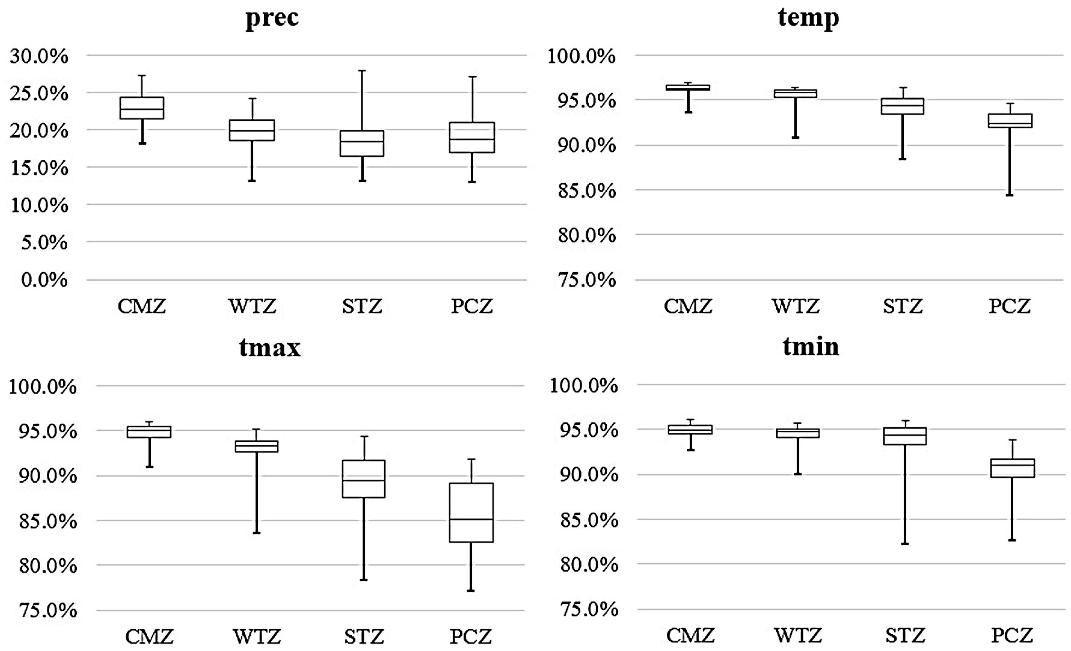
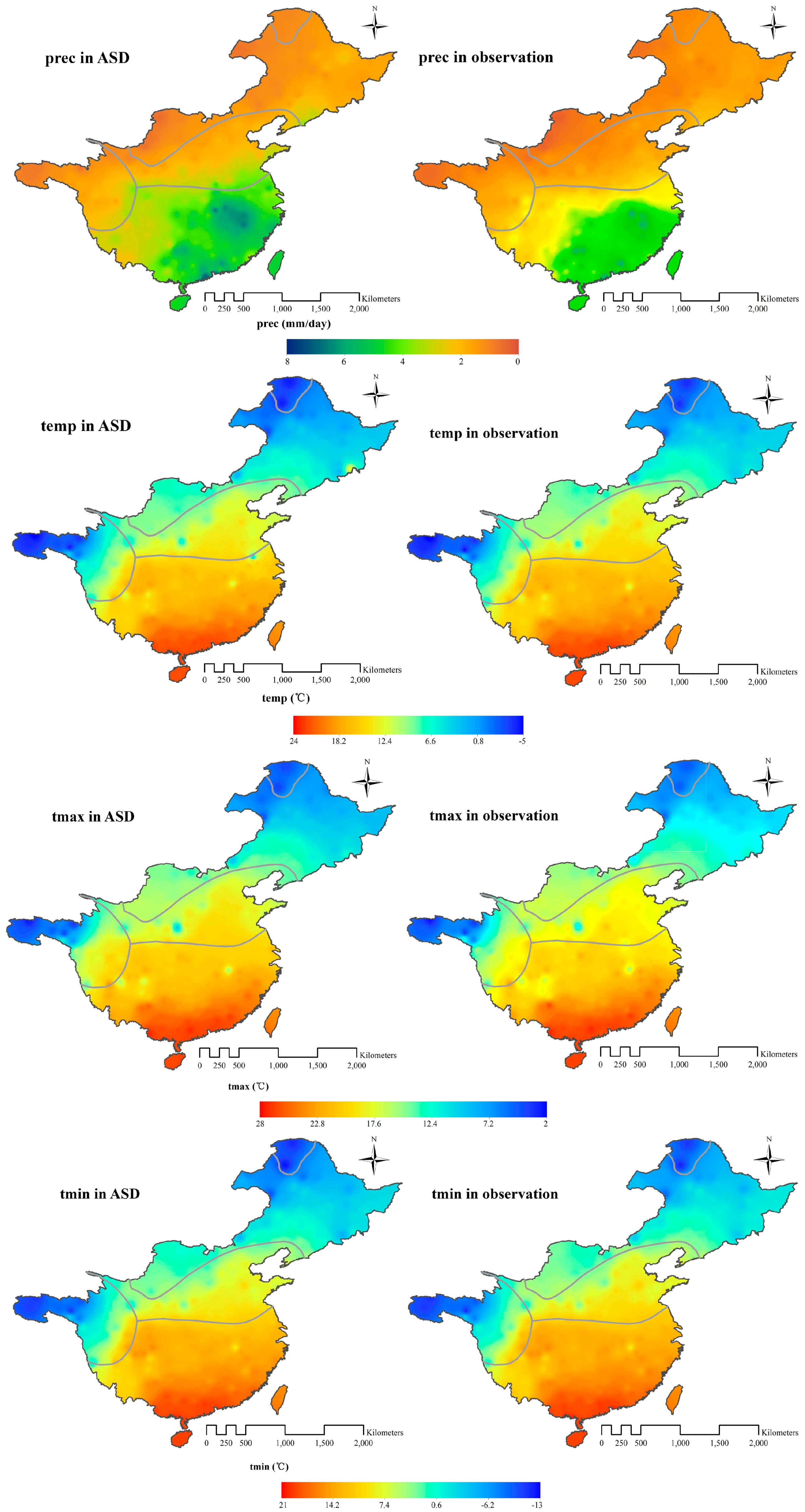
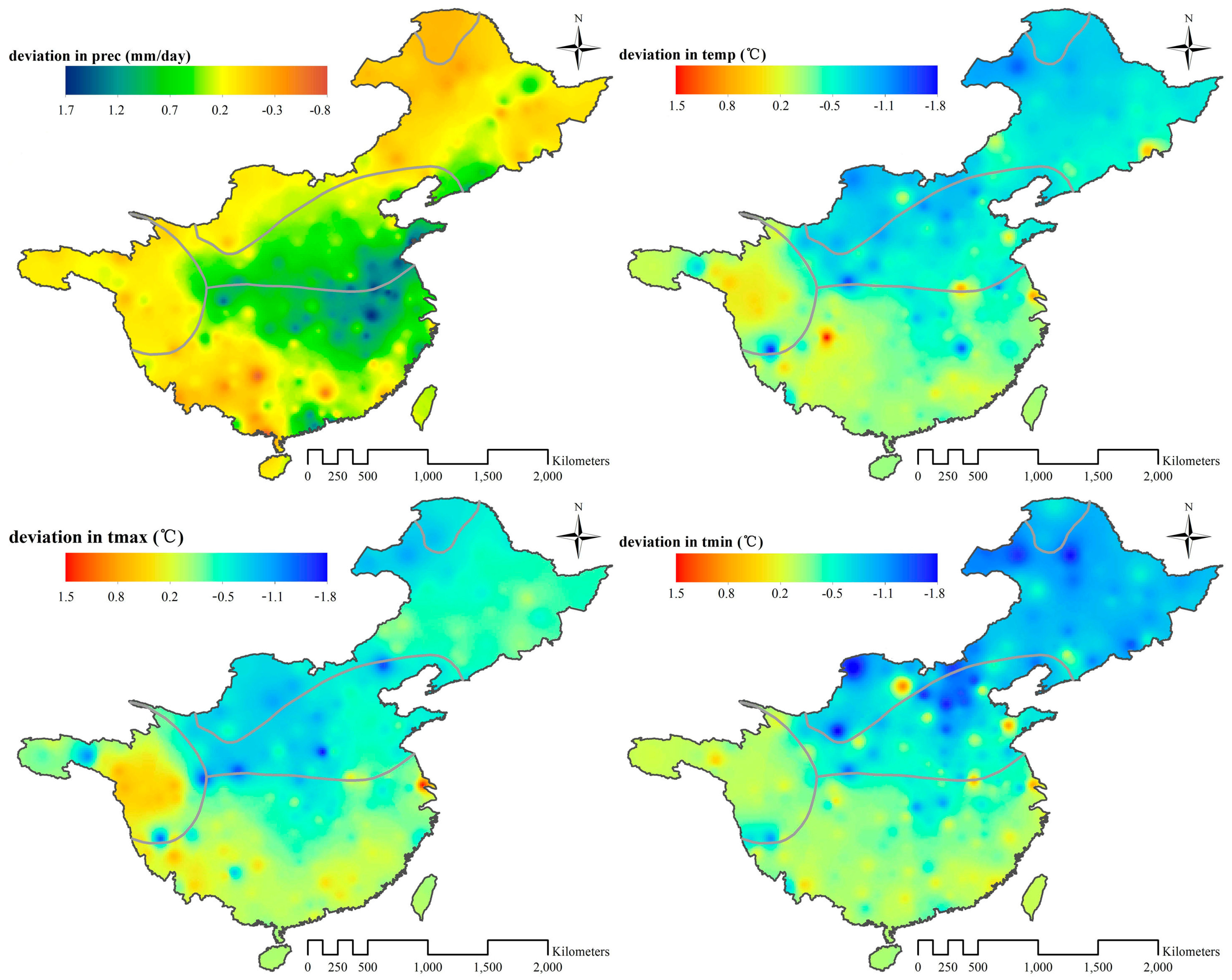
4.4. Validation of ASD

In this research, the validation period was from 1991 to 2005 (15 years total). To validate the ASD model, common evaluation indices such as the correlation coefficient (R) and normalized root mean standard error (NRMSE) were adopted to quantify the simulation results of the daily series in each zone. NRMSE is defined as the ratio of the root mean standard error and the standard error and can reflect the deviation of the simulation from the observation. A smaller value of NRMSE indicates higher simulation efficiency [28]. The results of the validation process shown in Table 3 indicate significant differences between the various zones. The correlation coefficient of the air temperature in the CMZ and the WTZ is larger than 0.8. The value of NRMSE is relatively low, suggesting optimal performance of the ASD model in the CMZ and the WTZ, which is in agreement with the calibration results. For the STZ and the PCZ, there was little difference in the values of R and NRMSE, except for the precipitation simulation, for which clear advantages were associated with the PCZ. The complicated topography may be the reason for the poorer performance of the ASD model in these two zones. Furthermore, the geographical position of the STZ results in greater influence of the monsoons in this zone, which made it more difficult for ASD to simulate the climatic variables with higher reliability.
According to the results of the significance test, all three temperature variables are consistently significant at the 95% and 99% confidence level, while the precipitation is not significant, which is beyond our expectation. As the precipitation is influenced by large-scale general circulations and complex local weather systems, the prediction of precipitation is always a difficult problem. However, only limited atmospheric circulation factors were considered to predict the precipitation in the ASD model. So the poor performance in the prediction of precipitation was presented in our study, which agrees well with the previous results [37,41].
To further validate the performance of simulated precipitation, the deviation (Er) and coefficient of determination (R2) for the probability of wet days and the mean rainfall of wet days were calculated between simulated precipitation and observations (listed in Table 4). The coefficient of determination is a measure used in statistical analysis that assesses how well a model explains and predicts future outcomes, and it measures the proportion of the variance in the dependent variable explained by the independent variable. R2 is usually used for the test in the goodness of fit. This coefficient is the quotient of the explained variation (sum of squares due to regression) to the total variation (total sum of squares), as follows:
r 2 = ( y ^ i y ¯ ) 2 ( y i y ¯ ) 2
where y i is the observation, y ¯ is the mean value of the observation, and y ^ i is the simulation. The coefficient of determination is represented as a value between zero and one. The closer the value is to one, the better the fit does (representing the fit between the ASD simulation and observation in our study).
It was found that simulated wet days in ASD were fewer than the observed wet days in the CMZ, with a negative deviation of 1.25%. The simulated mean rainfall of wet days in the CMZ is also lower than observed, with a negative deviation of 0.38%. The coefficients of determination for probability of wet days and mean rainfall of wet days consistently exceed 0.9. In the other three zones, the deviations of probability of wet days are positive and the simulated wet days were more than observed, ranging from 0.71% to 1.72%, and the coefficients of determination were between 0.839 and 0.897. The deviations of the mean rainfall of wet days vary from −0.17 to 1.05, and the coefficients of determination range from 0.861 to 0.910. We find that the ASD model can better capture the probability of wet days and the mean rainfall of wet days (the explained variances are consistently over than 0.839), although this model still has shortcomings in predicting the total amount of precipitation and its variability, which needs to further improve.
The spatial distribution of precipitation, mean air temperature, maximum air temperature, and minimum air temperature from both the observation data and the ASD output are exhibited in Figure 5. As seen in Figure 5, the gradient change of the precipitation and air temperature from southeast to northwest can be captured accurately by the ASD model, which indicates a strong spatial correlation of the ASD output.
Figure 6 plots the value of ASD simulation minus observation to indicate the differences between ASD simulation and observation data in the Eastern Monsoon Region of China. Combined with the data from the four zones, the deviations from the observed precipitation and air temperature by ASD were minor compared with the observations in the CMZ and the PCZ. The simulated precipitation deviations in these two zones are 8.64% and 5.99%, respectively; whereas in the WTZ and the STZ, the deviations are 14.79% and 23.16%, respectively. The simulated air temperatures in the CMZ and the WTZ are slightly lower than observation data by 0.15–0.89 °C; whereas in the STZ and the PCZ, the simulation values are higher by 0.01 to 0.40 °C for most stations. For the maximum air temperature and the minimum air temperature, higher simulation values have also been noted in the STZ and PCZ zones.
Generally, based on the statistical relationship between the large scale predictors and the local predictand developed in the calibration period, the ASD model is capable of simulating the air temperature. The simulation results of the precipitation, temporally and spatially, using the ASD model are also considered to be acceptable. Hence, the scenarios generated by the ASD model are reliable in the Eastern Monsoon Region of China.

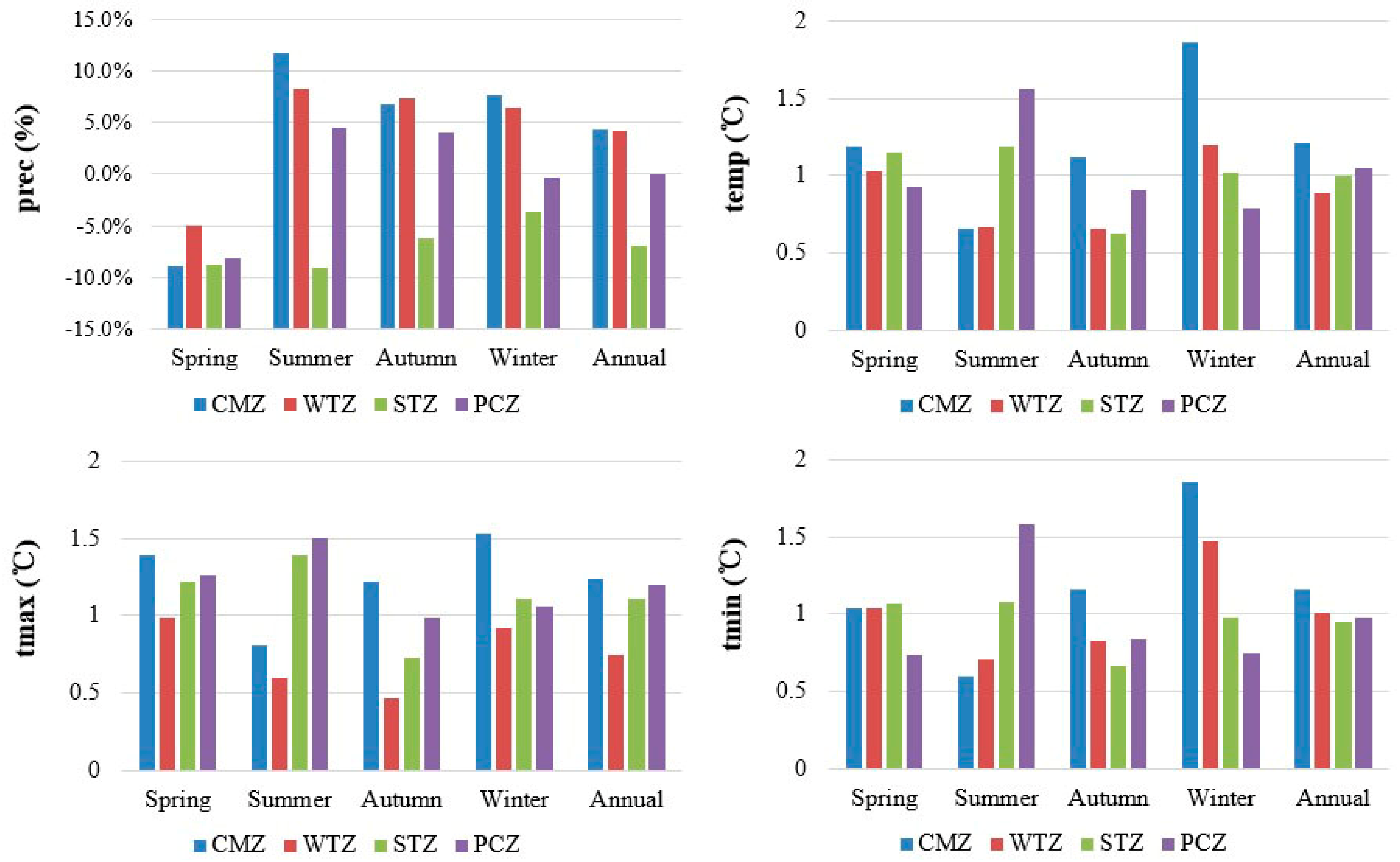
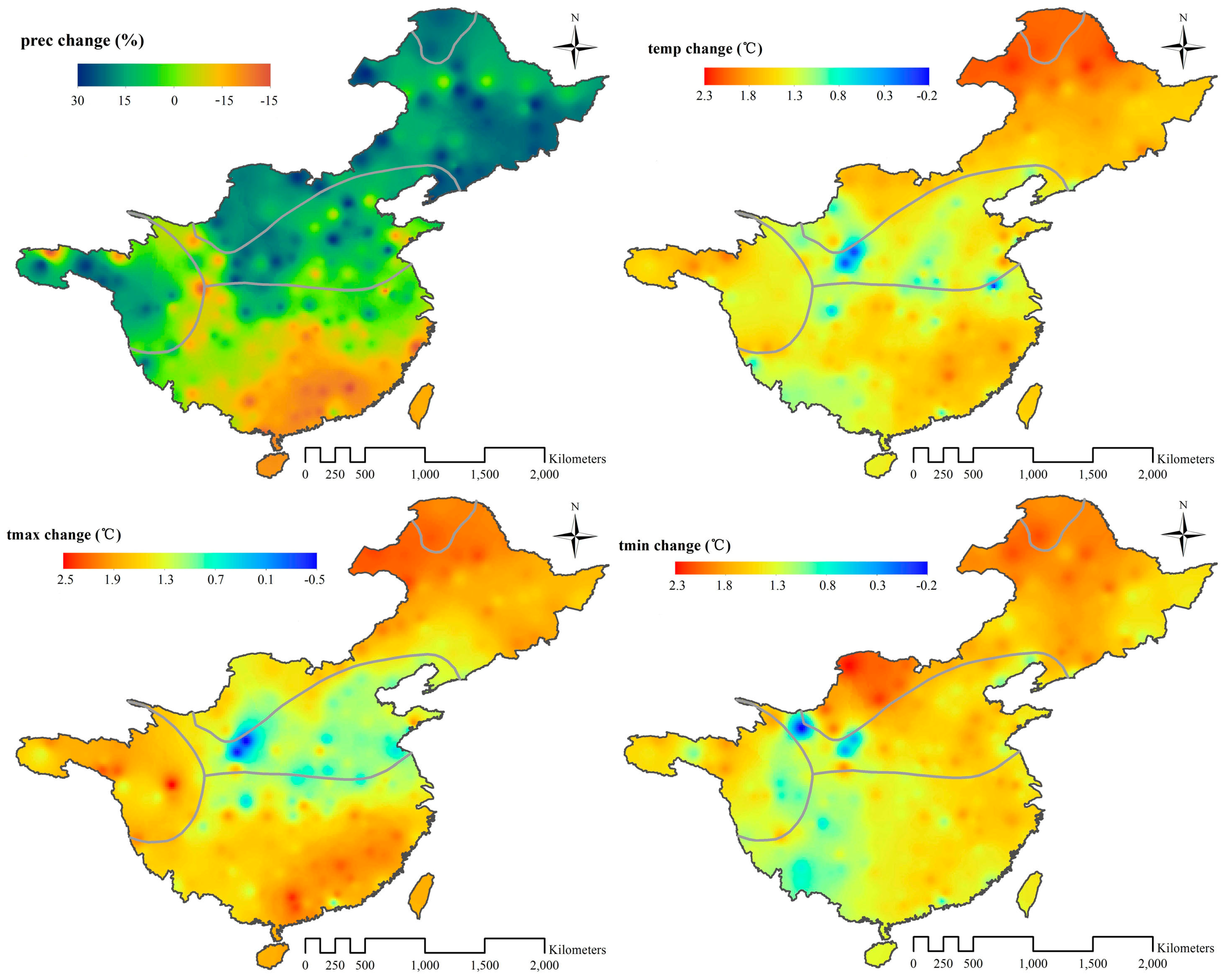
4.5. Generation of Climate Change Scenarios

Following the calibration and validation periods, the large scale meteorological variables from GCMs are downscaled through the ASD model. The seasonal and annual climate change scenarios (compared to the base period of 1991–2005) in the four zones during 2020–2050 are shown in Figure 7. The changes in the annual mean precipitation in the four zones (CMZ, WTZ, STZ, and PCZ) are 4.30%, 4.28%, −6.90%, and 0.02%, respectively. For the mean air temperature, the changes are 1.20, 0.89, 0.99 and 1.04 °C, respectively. The maximum (minimum) air temperature changes are 1.23 (1.16), 0.74 (1.01), 1.11 (0.95) and 1.20 °C (0.97 °C), respectively. The three air temperature variables at an annual scale in the four zones suggest an overall increase in the future. For precipitation, upward trends were found in both the CMZ and the WTZ, but in the STZ a strong downward trend was detected.
The change of the seasonal scenarios in the four zones exhibited obvious differences. For precipitation, the values for future precipitation in the spring in the four zones all decreased by 5–10%. The reduction of spring precipitation in the past has been detected [42], and the reduction trend in the future in relevant areas has been projected [43]. The projection of lower precipitation in spring in parts of China may be explainable. In the other seasons, precipitation shows an upward trend, except in the STZ. For the air temperature, the values for seasonal change of the three air temperature variables in the four zones all exhibited rising trends, with an increase in the range of 0.59–1.85 °C. Compared with the maximum air temperature, the change of the temporal sequence in the minimum air temperature was more similar to the mean air temperature. The most significant upward trend was detected in the CMZ and the STZ. Given that precipitation in the STZ will decrease, the increasing evapotranspiration level due to the higher air temperature would aggravate water scarcity in this zone.
The spatial distribution of the future changes of four variables in four zones was drawn using GIS. The results are shown in Figure 8, from which we can see a significant spatial difference in the changes. For precipitation, the annual mean precipitation in most of the STZ would decrease, especially in the southeastern area, where the decrease would be nearly 28%. In the CMZ and in most of the WTZ and PCZ, the future precipitation would increase by 0–29.8%, whereas the spatial distribution of the change in the maximum air temperature was more similar to the mean air temperature. For these two variables, remarkable downward trends were detected in the WTZ, whereas, in the PCZ and most of the STZ and CMZ, the trends were upward. In the northern area of the CMZ and in the southeastern area of the STZ, the upward trends were more remarkable, with increases of 1.5–2.5 °C. Consistent with the result derived from the change of the temporal sequence, precipitation in the southeastern area of the STZ will tend to decrease in the future. Meanwhile, the air temperature in this region will increase in the future, which would lead to more evapotranspiration. These two factors may result in a worsening of the water resource situation.

5. Methodological Limitations

In this study, only the ensemble mean of all models was downscaled based on the evaluation (shown in Figure 2). It is clear that there is significant uncertainty among models, and it is necessary to take this uncertainty into consideration. A study exploring uncertainty in GCMs as well as in the ASD model is an area of future research. Among the four greenhouse gas emission scenarios, only the medium scenario RCP4.5 was adopted in our study, but in the future it would be useful to introduce other scenarios (such as RCP 8.5, RCP 6.0, RCP 2.6). This will allow a comprehensive comparison to explore what would happen for other scenarios. Due to the calculation burden and time constraints, other scenarios were not considered in this research.

6. Conclusions

The evaluation results indicate that the GCMs perform differently over the Eastern Monsoon Region of China. Overall, the GCMs ensembles are superior to the single model, and the simple averaging ensemble surpasses the weighted averaging ensembles. MGCMs were capable of depicting the annual trends and spatial distribution of the climatic variables; however, MGCMs exhibit poorer performance in simulating exceedingly high or low values of variables, which is due to the simple averaging process, wherein extreme values were averaged out. Considering the purpose of this research, the output of MGCMs can be used to describe seasonal and annual climate change trends, as well as spatial distribution in future scenarios. However, in other research studies for extreme climatic events, it is considered essential to explore other methods.
In the process of predictor selection, different local variables, such as precipitation amount and air temperature in different zones, were related to various atmospheric predictors. From a spatial perspective, the selected predictors vary from zone to zone. Generally, ta500, tas, and zg500 are the most significant predictors for the four variables in the four temperate zones. Simultaneously, due to the different latitudes, the influence of uas becomes weaker from the CMZ to the STZ.
During calibration and validation, ASD behaves better in simulating the air temperature than the precipitation amount. For air temperature, the explained variances in the CMZ are greater than 91.0%, whereas the explained variances for precipitation are 13.0–28.0%, even in the CMZ, where, despite relatively better simulation being observed, the median value of explained variance was only 22.8%. Compared to other related research, this simulation efficiency for precipitation downscaling is acceptable. In view of the different temperate zones, the further north the zone is located, the higher the effectiveness of the model. The optimal performance of ASD was achieved in the CMZ and in the WTZ, which may be due to the complicated topography and the geographical position of these two zones. Overall, the ASD method was adaptable to the Eastern Monsoon Region of China.
The projection of future scenarios from 2020 to 2050 showed that air temperature and air temperature extremes in most areas of the four zones would exhibit upward trends in the future in the range of 0–2.5 °C. For precipitation, clear decreasing trends were detected in the spring and in the STZ. In the other seasons and zones, upward trends were found of less than 30%. Notably, from the temporal trends analysis, compared with the maximum air temperature, the change of the temporal sequence of the minimum air temperature was more similar to the mean air temperature. However, from the characteristics of the spatial distribution, the change pattern of the maximum air temperature was more similar to the mean air temperature. From the spatial distribution of the climate change scenarios, precipitation in the southeastern area of the STZ will decline in the future, whereas the air temperature (especially the maximum air temperature) in this region will increase, which may result in a worsening of the water resource situation in the area. Such a trend would negatively impact agricultural production and the overall ecological environment. In such cases therefore, it would be necessary to suitably implement water management strategies to reduce the potential risks.

Acknowledgments

This study was financially supported by the Major State Basic Research Development Program of China (973 Program) (No. 2010CB428402) and the National Natural Science Foundation of China (No. 91647202 and No. 41405076). We would like to thank the National Climatic Centre (NCC) of the China Meteorological Administration (CMA) in Beijing for providing valuable data.

Author Contributions

All authors contributed to the design and development of this manuscript. Pin Liu carried out the modeling work and data analysis and prepared the first draft of the manuscript. Zongxue Xu is the graduate advisor of Pin Liu and contributed many ideas to the study. Xiuping Li provided important advice on the concept of methodology.

Conflicts of Interest

The authors declare no conflict of interest.

References

  1. Intergovernmental Panel on Climate Change (IPCC). Climate Change 2013: The Physical Science Basis; Contribution of Working Group I to the Fifth Assessment Report of the Intergovern-Mental Panel on Climate Change; Cambridge University Press: Cambridge, UK; New York, NY, USA, 2013. [Google Scholar]
  2. Gebremeskel, S.; Liu, Y.B.; de Smedt, F.; Hoffmann, L.; Pfister, L. Analysing the effect of climate changes on streamflow using statistically downscaled GCM scenarios. Int. J. River Basin Manag. 2005, 2, 271–280. [Google Scholar] [CrossRef]
  3. Ahmadalipour, A.; Rana, A.; Moradkhani, H.; Sharma, A. Multi-criteria evaluation of CMIP5 GCMS for climate change impact analysis. Theor. Appl. Climatol. 2015, 1–17. [Google Scholar] [CrossRef]
  4. Wilby, R.L.; Hay, L.E.; Gutowski, W.J.; Arritt, R.W.; Takle, E.S.; Pan, Z.; Leavesley, G.H.; Martyn, P.C. Hydrological responses to dynamically and statistically downscaled climate model output. Geophys. Res. Lett. 2000, 27, 1199–1202. [Google Scholar] [CrossRef]
  5. Gädeke, A.; Hölzel, H.; Koch, H.; Pohle, I.; Grünewald, U. Analysis of uncertainties in the hydrological response of a model-based climate change impact assessment in a subcatchment of the Spree River, Germany. Hydrol. Process. 2014, 28, 3978–3998. [Google Scholar] [CrossRef]
  6. Xu, C.Y. From GCMs to river flow: A review of downscaling methods and hydrologic modeling approaches. Prog. Phys. Geog. 1999, 23, 229–249. [Google Scholar] [CrossRef]
  7. Chu, J.; Xia, J.; Xu, C.Y.; Singh, V. Statistical downscaling of daily mean temperature, pan evaporation and precipitation for climate change scenarios in Haihe River, China. Theor. Appl. Climatol. 2010, 99, 149–161. [Google Scholar] [CrossRef]
  8. Khattak, M.S.; Babel, M.S.; Sharif, M. Hydro-meteorological trends in the Upper Indus River basin in Pakistan. Clim. Res. 2011, 46, 103–119. [Google Scholar] [CrossRef]
  9. Zhang, X.C.; Liu, W.Z.; Li, Z.; Chen, J. Trend and uncertainty analysis of simulated climate change impacts with multiple GCMS and emission scenarios. Agric. For. Meteorol. 2011, 151, 1297–1304. [Google Scholar] [CrossRef]
  10. Fowler, H.J.; Wilby, R.L. Beyond the downscaling comparison study. Int. J. Climatol. 2007, 27, 1543–1545. [Google Scholar] [CrossRef]
  11. Casanueva, A.; Herrera, S.; Fernández, J.; Gutiérrez, J.M. Towards a fair comparison of statistical and dynamical downscaling in the framework of the EURO-CORDEX initiative. Clim. Chang. 2016, 137, 411–426. [Google Scholar] [CrossRef]
  12. Boé, J.; Terray, L.; Habets, F.; Martin, E. Statistical and dynamical downscaling of the seine basin climate forhydro-meteorological studies. Int. J. Climatol. 2007, 27, 1643–1655. [Google Scholar] [CrossRef]
  13. Nover, D.M.; Witt, J.W.; Butcher, J.B.; Johnson, T.E.; Weaver, C.P. The effects of downscaling method on thevariability of simulated watershed response to climate change in five us basins. Earth Interact. 2016, 20, 1–27. [Google Scholar] [CrossRef]
  14. Wilby, R.L.; Wigley, T.M.L. Downscaling general circulation model output: A review of methods and limitations. Prog. Phys. Geogr. 1997, 21, 530–548. [Google Scholar] [CrossRef]
  15. Gutmann, E.D.; Rasmussen, R.M.; Liu, C.H. A comparison of statistical and dynamical downscaling of winter precipitation over complex terrain. J. Clim. 2012, 25, 262–281. [Google Scholar] [CrossRef]
  16. Kim, S.; Noh, H.; Jung, J. Assessment of the Impacts of Global Climate Change and Regional Water Projects on Streamflow Characteristics in the Geum River Basin in Korea. Water 2016, 8, 91. [Google Scholar] [CrossRef]
  17. Bergström, S.; Carlsson, B.; Gardelin, M. Climate change impacts on runoff in Sweden: Assessment by global climate models, dynamic downscaling and hydrological model. Clim. Res. 2001, 16, 101–112. [Google Scholar] [CrossRef]
  18. Xue, Y.; Vasic, R.; Janjic, Z. Assessment of Dynamic Downscaling of the Continental U.S. Regional Climate Using the Eta/SSiB Regional Climate Model. J. Clim. 2007, 20, 4172–4193. [Google Scholar] [CrossRef]
  19. Wilby, R.L.; Wigley, T.M.L.; Conway, D. Statistical downscaling of general circulation model output: A comparison of methods. Water Resour. Res. 1998, 34, 2995–3008. [Google Scholar] [CrossRef]
  20. Fan, L.J. Preliminary study of statistically downscaled temperature ensemble predictions in eastern China. Plateau Meteorol. 2010, 29, 392–402. [Google Scholar]
  21. Liu, J.; Yuan, D.; Zhang, L. Comparison of Three Statistical Downscaling Methods and Ensemble Downscaling Method Based on Bayesian Model Averaging in Upper Hanjiang River Basin, China. Adv. Meteorol. 2016, 2016, 1–12. [Google Scholar] [CrossRef]
  22. Zhang, X.; Yan, X. A new statistical precipitation downscaling method with Bayesian model averaging: A case study in China. Clim. Dynam. 2015, 45, 1–15. [Google Scholar] [CrossRef]
  23. Feddersen, H.; Andersen, U. A method for statistical downscaling of seasonal ensemble predictions. Tellus A 2005, 57, 398–408. [Google Scholar] [CrossRef]
  24. Zorita, E.; Storch, H.V. The Analog Method as a Simple Statistical Downscaling Technique: Comparison with More Complicated Methods. J. Clim. 1999, 12, 2474–2489. [Google Scholar] [CrossRef]
  25. Tatli, H.; Dalfes, H.N.; Menteş, Ş.S. A statistical downscaling method for monthly total precipitation over Turkey. Int. J. Climatol. 2004, 24, 161–180. [Google Scholar] [CrossRef]
  26. Chen, Y.D.; Chen, X.; Xu, C.Y.; Shao, Q. Downscaling of daily precipitation with a stochastic weather generator for the subtropical region in South China. Hydrol. Earth. Syst. Sci. Discuss. 2006, 3, 1145–1183. [Google Scholar] [CrossRef]
  27. Zhao, F.F.; Xu, Z.X. Comparative analysis on downscaled climate scenarios for headwater catchment of Yellow River using sds and delta methods. Acta Meteorol. Sin. 2007, 65, 653–662. [Google Scholar]
  28. Huang, J.X.; Xu, Z.X.; Liu, Z.F.; Zhao, F.F. Analysis of future climate change in the Taihu Basin using statistical downscaling. Resour. Sci. 2008, 30, 1811–1817. [Google Scholar]
  29. Liu, Z.F.; Xu, Z.X. Trends of daily extreme air temperature in the Wei River Basin in the future. Resour. Sci. 2009, 31, 1573–1580. [Google Scholar]
  30. Liu, P.; Xu, Z.X.; Li, X.P.; Wang, S.Z. Application of ASD Statistical Technique in Typical Basins of the Eastern monsoon region in China. J. Chin. Hydrol. 2013, 33, 1–9. [Google Scholar]
  31. Mcsweeney, C.F.; Jones, R.G.; Lee, R.W. Selecting CMIP5 GCMs for downscaling over multiple regions. Clim. Dynam. 2014, 44, 3237–3260. [Google Scholar] [CrossRef]
  32. Taylor, K.E. Summarizing multiple aspects of model performance in a single diagra. J. Geophys. Res. 2001, 106, 7183–7192. [Google Scholar] [CrossRef]
  33. Hessami, M.; Gachon, P.; Ouarda, T. Automated regression-based statistical downscaling tool. Environ. Model. Softw. 2008, 23, 813–834. [Google Scholar] [CrossRef]
  34. Mahmood, R.; Jia, S. Assessment of Impacts of Climate Change on the Water Resources of the Transboundary Jhelum River Basin of Pakistan and India. Water 2016, 8, 246. [Google Scholar] [CrossRef]
  35. Wilby, R.L.; Wigley, T.M. Precipitation predictor for downscaling: Observed and general circulation model relationships. Int. J. Climatol. 2000, 20, 641–661. [Google Scholar] [CrossRef]
  36. Wilby, R.L.; Tomlinson, O.J.; Dawson, C.W. Multi-site simulation of precipitation by conditional resampling. Clim. Res. 2003, 23, 183–194. [Google Scholar] [CrossRef]
  37. Wilby, R.L.; Dawson, C.W.; Barrow, E.M. SDSM-A decision support tool for the assessment of regional climate change impacts. Environ. Model. Softw. 2002, 17, 147–159. [Google Scholar] [CrossRef]
  38. Liu, L.L.; Liu, Z.F.; Xu, Z.X. Trends of climate change for the upper-middle reaches of the yellow river in the 21st century. Adv. Clim. Chg. Res. 2008, 4, 167–172. [Google Scholar]
  39. Chen, W.L. Projection and Evaluation of the Precipitation Extremes Indices over China. Master’s Thesis, Nanjing University of Information Science & Technology, Nanjing, China, 2008. [Google Scholar]
  40. Liu, L.; Xu, Z.X.; Huang, J.X. Comparative study on the application of two downscaling methods in the Taihu Basin. J. Meteorol. Sci. 2011, 31, 160–169. [Google Scholar]
  41. Huang, J.; Zhang, J.C.; Zhang, Z.X.; Xu, C.Y.; Wang, B.L.; Yao, J. Estimation of future precipitation change in the Yangtze River basin by using statistical downscaling method. Stoch. Env. Res. Risk Assess. 2011, 25, 781–792. [Google Scholar] [CrossRef]
  42. Hu, Y.J.; Zhu, Y.M.; Zhong, Z.; Zhang, H.J. Estimation of Precipitation in Two Climate Change Scenarios in China. Plateau Meteorol. 2013, 32, 778–786. [Google Scholar]
  43. Sun, J.L.; Lei, X.H.; Jiang, Y.Z.; Wang, H. Variation Trend Analysis of Meteorological Variables and Runoff in Upper Reaches of Yangtze River. Int. J. Hydroelectr. Energy 2012, 30, 1–4. [Google Scholar]
Figure 1. The location of gauging stations in the Eastern Monsoon Region.
Water 09 00305 g001
Figure 2. Rank scores of GCM models for precipitation and mean air temperature simulation.
Water 09 00305 g002
Figure 3. Percentage of selected predictors in different temperate zones (Note: 1-hus500; 2-hus850; 3-slp; 4-ta500; 5-ta850; 6-tas; 7-ua850; 8-uas; 9-zg500; 10-zg700; 11-zg850. prec: precipitation; temp: mean air temperature; tmax: maximum air temperature; tmin: minimum air temperature).
Water 09 00305 g003
Figure 4. Explained variance of Automated Statistical Downscaling (ASD) output in four temperature zones.
Water 09 00305 g004
Figure 5. Spatial distribution of variables in observation data and ASD outputs during validation. (Note: maps on the two columns refer to ASD simulations and observation data, respectively; maps from top to bottom present precipitation, mean air temperature, maximum air temperature, and minimum air temperature in sequence).
Water 09 00305 g005
Figure 6. Difference between ASD simulation and observation. (Note: maps from left to right and from top to bottom present precipitation, mean air temperature, maximum air temperature, and minimum air temperature, respectively).
Water 09 00305 g006
Figure 7. Seasonal and annual mean climate changes during 2020–2050 under the scenario of RCP4.5.
Water 09 00305 g007
Figure 8. Spatial distribution of climate change during 2020–2050 under scenario RCP4.5. (Note: maps from left to right and from top to bottom present precipitation, mean air temperature, maximum air temperature, and minimum air temperature, respectively).
Water 09 00305 g008
Table 1. Detailed information of 19 General Circulation Models (GCMs).
No.ModelInstitutionNationResolution
1ACCESS1.3Commonwealth Scientific and Industrial Research Organization and Bureau of MeteorologyAustralia145 × 192
2BCC-CSM1.1Beijing Climate Center, China Meteorological AdministrationChina64 × 128
3BNU-ESMCollege of Global Change and Earth System Science, Beijing Normal UniversityChina64 × 128
4CanESM2Canadian Centre for Climate Modelling and AnalysisCanada64 × 128
5CCSM4National Center for Atmospheric ResearchAmerica192 × 288
6CMCC-CESMCentro Euro-Mediterraneo per I Cambiamenti ClimaticiEurope48 × 96
7CNRM-CM5Centre National de Recherches Météorologiques/Centre Européen de Recherche et Formation Avancée en Calcul ScientifiqueFrance128 × 256
8CSIRO-Mk3.6.0Commonwealth Scientific and Industrial Research Organization in collaboration with Queensland Climate Change Centre of ExcellenceAustralia96 × 192
9EC-EARTHEC-EARTH consortiumEurope160 × 320
10FGOALS-g2LASG, Institute of Atmospheric Physics, Chinese Academy of Sciences and CESS,Tsinghua UniversityChina60 × 128
11GFDL-CM3NOAA Geophysical Fluid Dynamics LaboratoryAmerica90 × 144
12GISS-E2-RNASA Goddard Institute for Space StudiesAmerica90 × 144
13HadGEM2-AONational Institute of Meteorological Research/Korea Meteorological AdministrationKorea145 × 192
14HadGEM2-CCMet Office Hadley Centre England145 × 192
15INMCM4Institute for Numerical MathematicsRussia120 × 180
16IPSL-CM5A-LRInstitut Pierre-Simon LaplaceFrance96 × 96
17MIROC-ESMJapan Agency for Marine-Earth Science and Technology, Atmosphere and Ocean Research Institute (The University of Tokyo), and National Institute for Environmental StudiesJapan64 × 128
18MPI-ESM-LRMax Planck Institute for MeteorologyGermany96 × 192
19NorESM1-MNorwegian Climate CentreNorway96 × 144
Table 2. Comparison of explained variance in different downscaling research.
ScholarResearch AreaPercentage of Explained Variance (%)
PrecipitationMean Air TemperatureMaximum Air TemperatureMinimum Air Temperature
Zhao and Xu [27]Source of Yellow River Basin7.00–25.3 49.5–55.423.8–27.51
Liu et al. [38]Upper-middle reaches of Yellow River8.0–20.0 63.0–69.0>64.0
Chu et al. [7]Hai River Basin 99.36–99.64
Chen [39]Yangtze-Huaihe River Basin8.8–20.6
Liu and Xu [29]Wei River Basin 70.8–89.163.8–8601
Liu et al. [40]Taihu Basin20.8–33.0 70.1–80.175.4–84.5
This researchEastern monsoon region, China13.0–27.984.5–97.077.1–96.182.2–96.1
Table 3. Comparison of evaluation indices in four temperate zones.
ZonesPrecipitationMean Air TemperatureMaximum Air TemperatureMinimum Air Temperature
RNRMSERNRMSERNRMSERNRMSE
CMZ0.47 *1.300.90 ***0.460.87 ***0.550.89 ***0.48
WTZ0.391.400.89 ***0.500.80 ***0.660.88 ***0.51
STZ0.241.470.80 ***0.620.70 ***0.790.83 ***0.59
PCZ0.331.350.84 ***0.570.70 ***0.800.83 ***0.58
Notes: * represents 90% confidence level; ** represents 95% confidence level; *** represents 99% confidence level.
Table 4. Er and R2 of the probability of wet days and the average rainfall of wet days.
ZonesProbability of Wet DaysMean Rainfall of Wet Days
Er (%)R2Er (mm/Day)R2
CMZ−1.250.906−0.380.923
WTZ1.450.8970.620.910
STZ0.710.8721.050.874
PCZ1.720.839−0.170.861

