
Changes of Reference Evapotranspiration and Its Relationship to Dry/Wet Conditions Based on the Aridity Index in the Songnen Grassland, Northeast China


Abstract
:1. Introduction
2. Materials and Methods
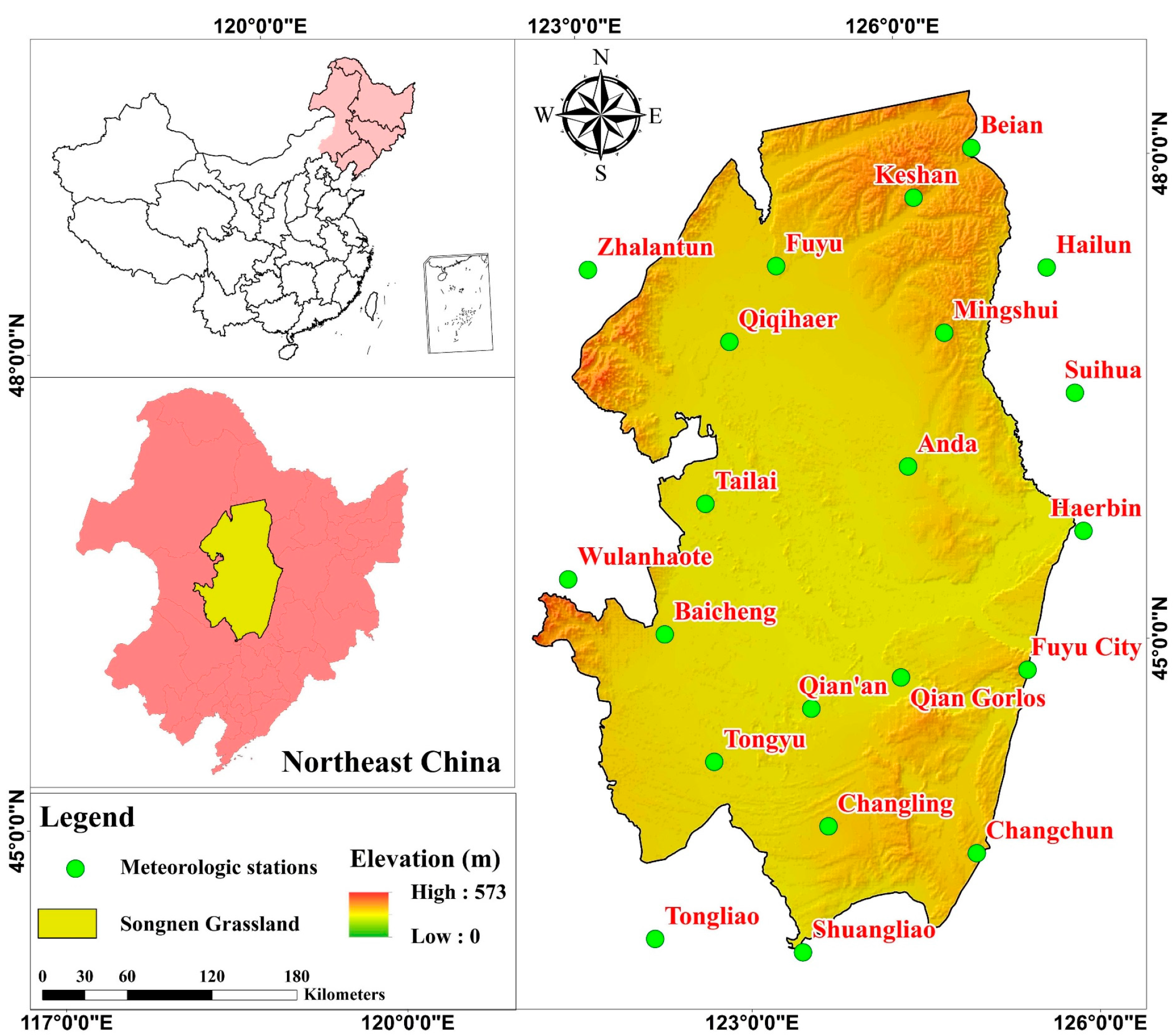
2.1. Study Area
2.2. Climate Data and Quality Control
2.3. Methods
2.3.1. Calculation of Reference Evapotranspiration (ET0)
2.3.2. Trend Analysis
2.3.3. Sensitivity Analysis
2.3.4. Aridity Index (AI Index)
2.3.5. Spatial Interpolation
3. Results
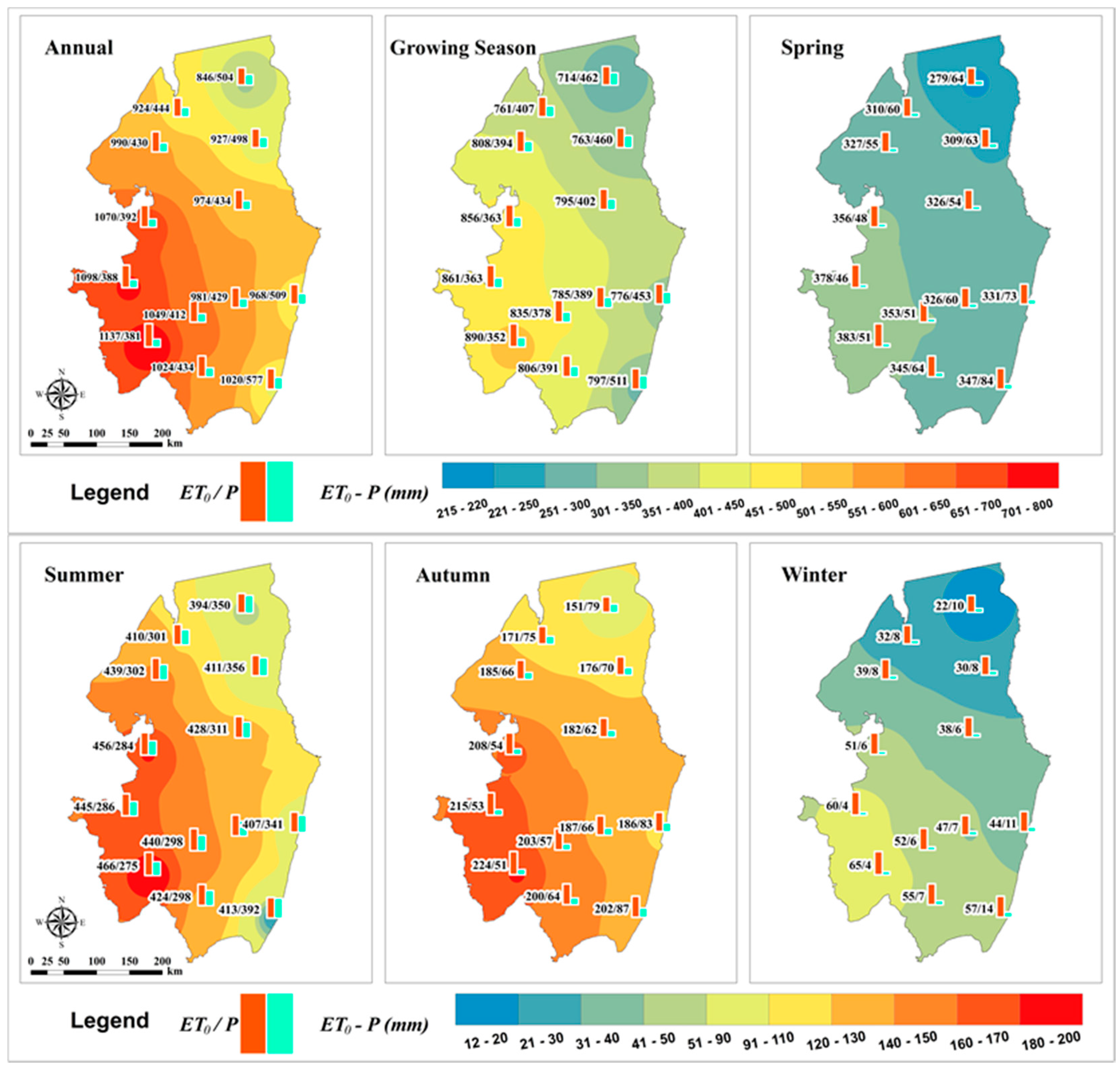
3.1. Spatial Distribution of ET0, P, and Their Difference over the Period from 1960–2014
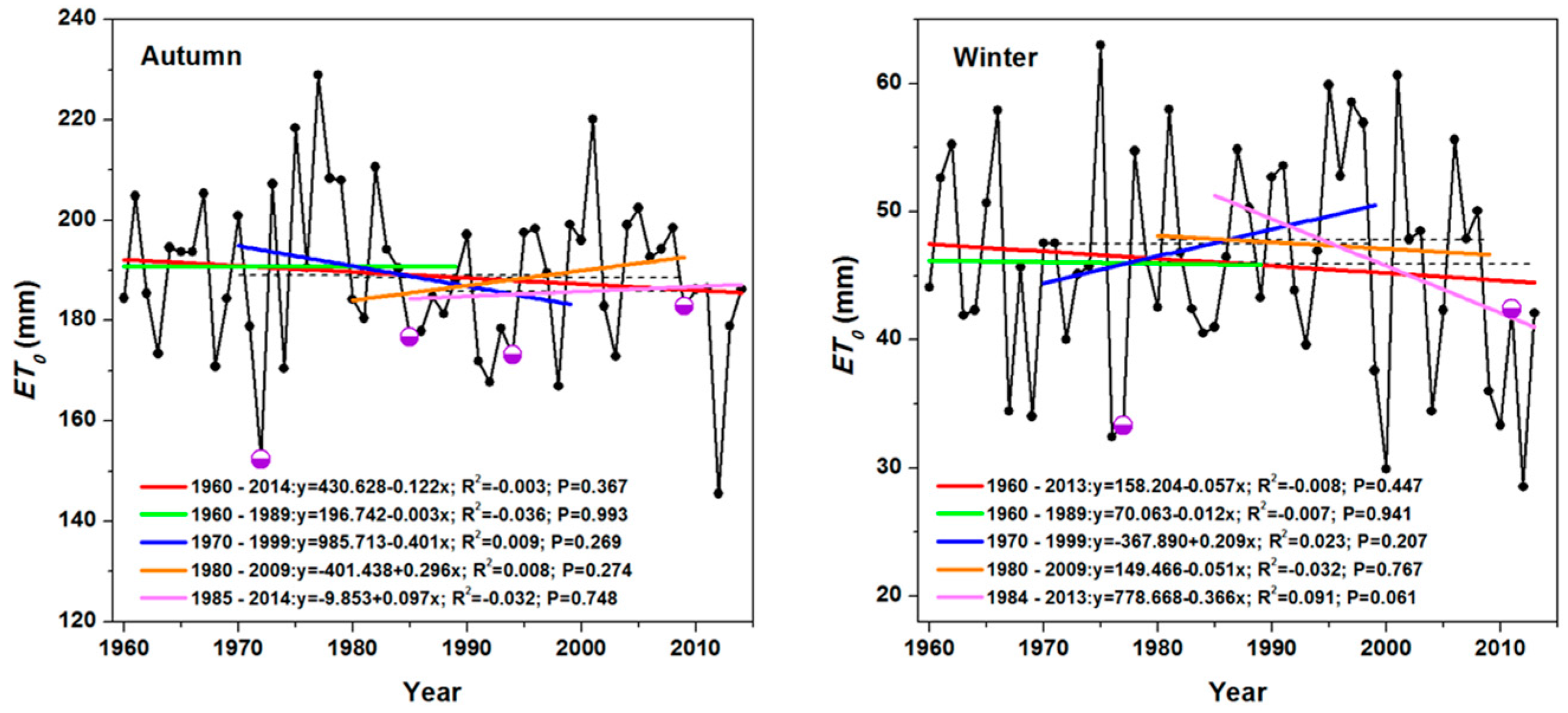
3.2. Temporal Variations of ET0
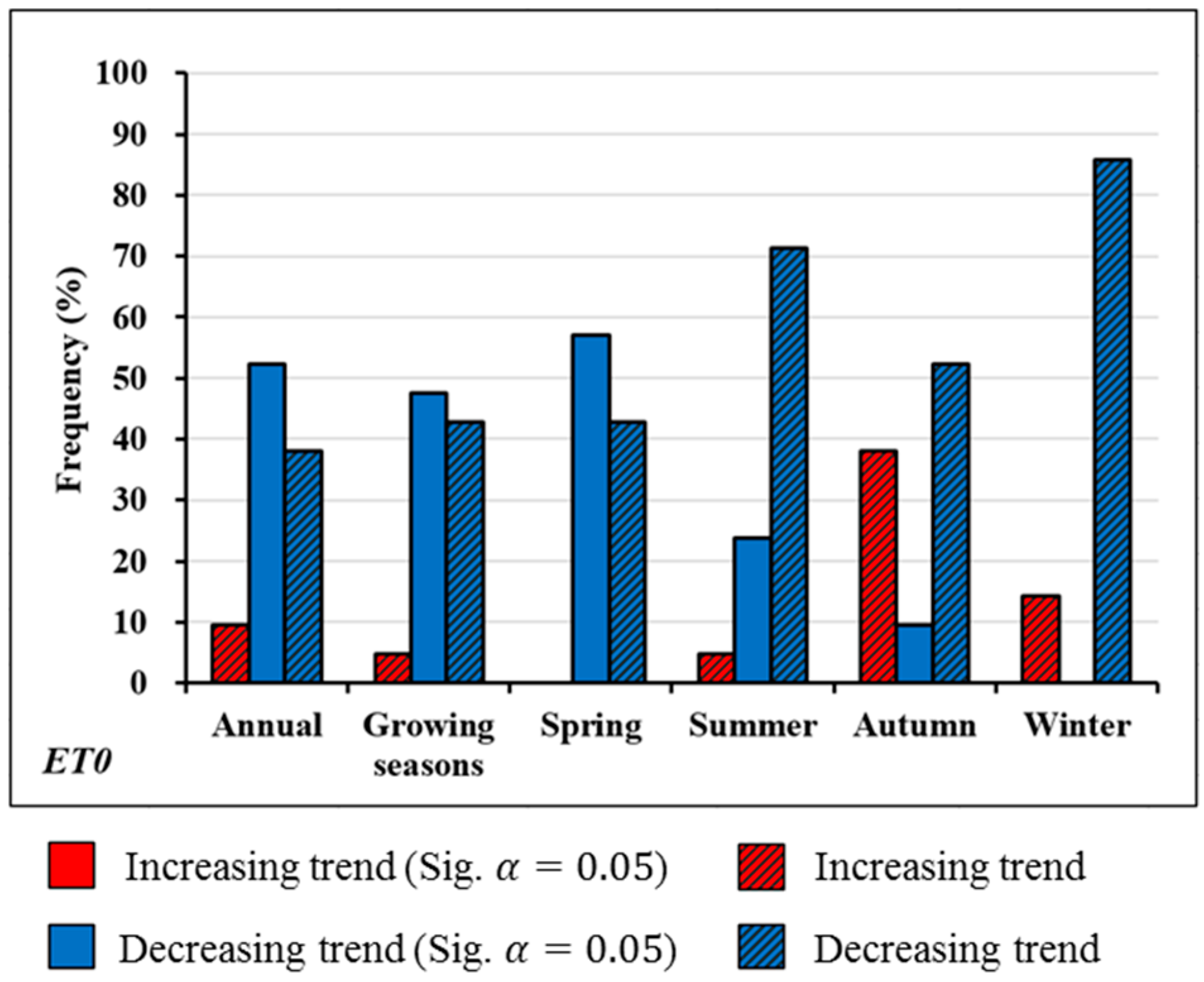
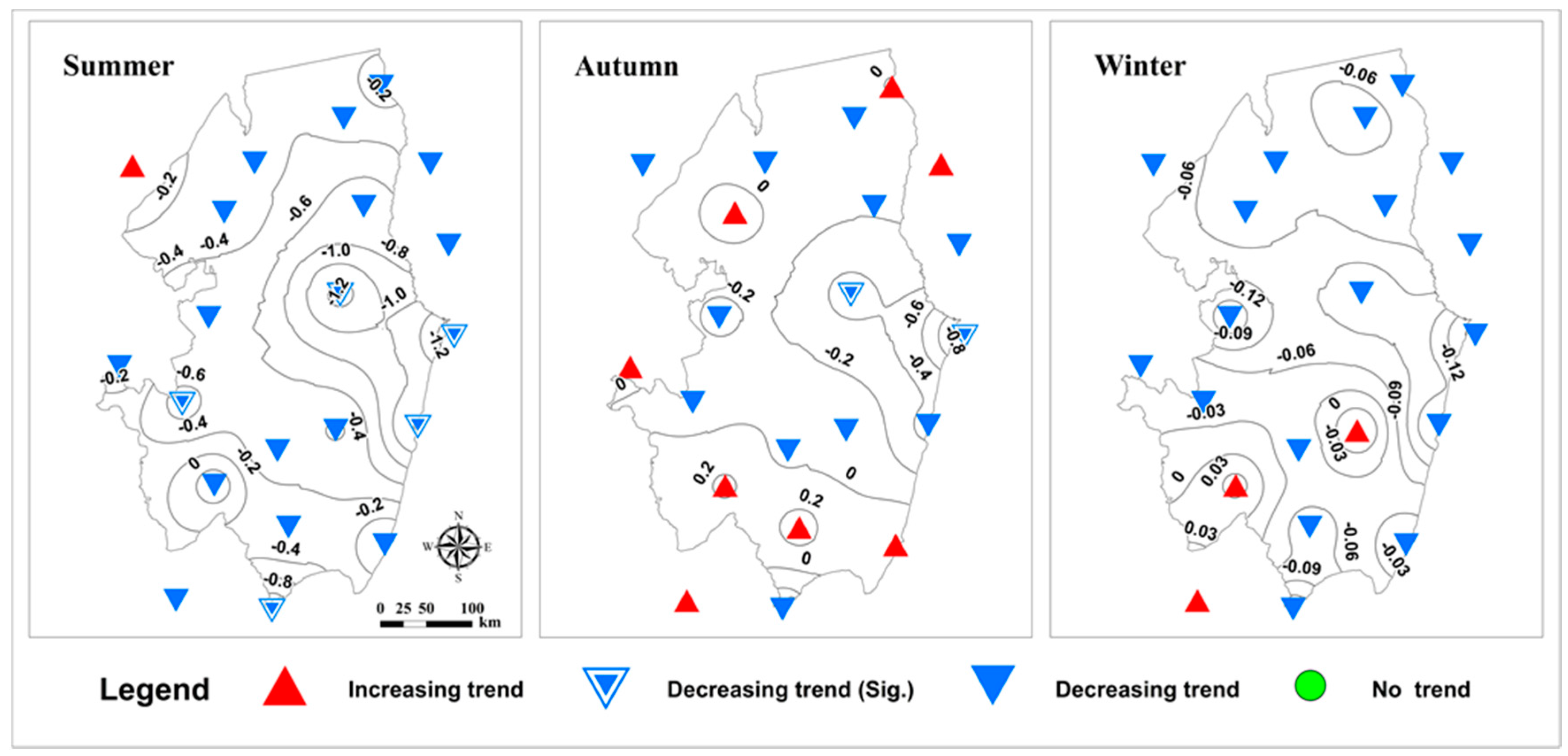
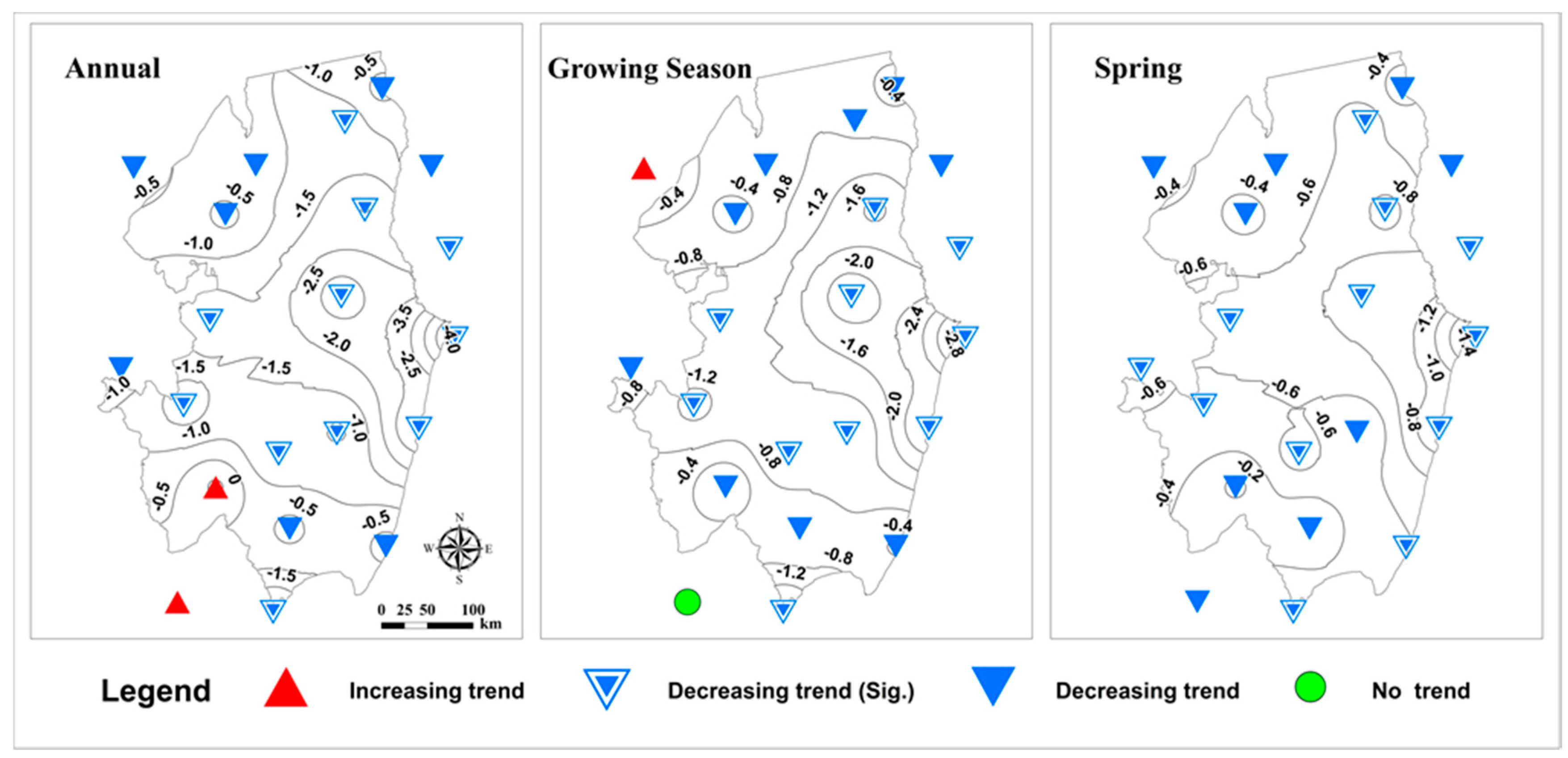
3.3. Spatial Patterns of Trends in ET0
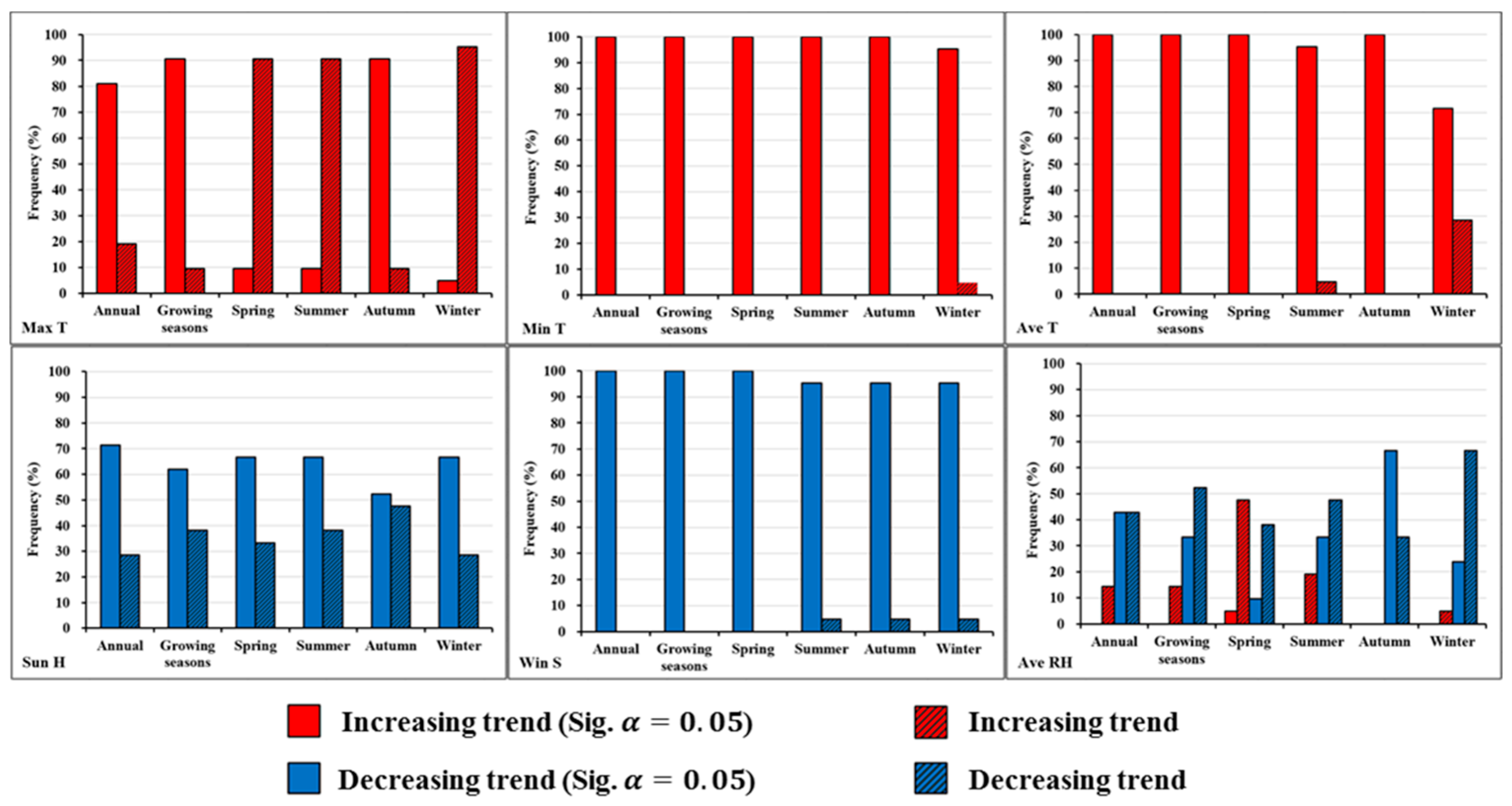
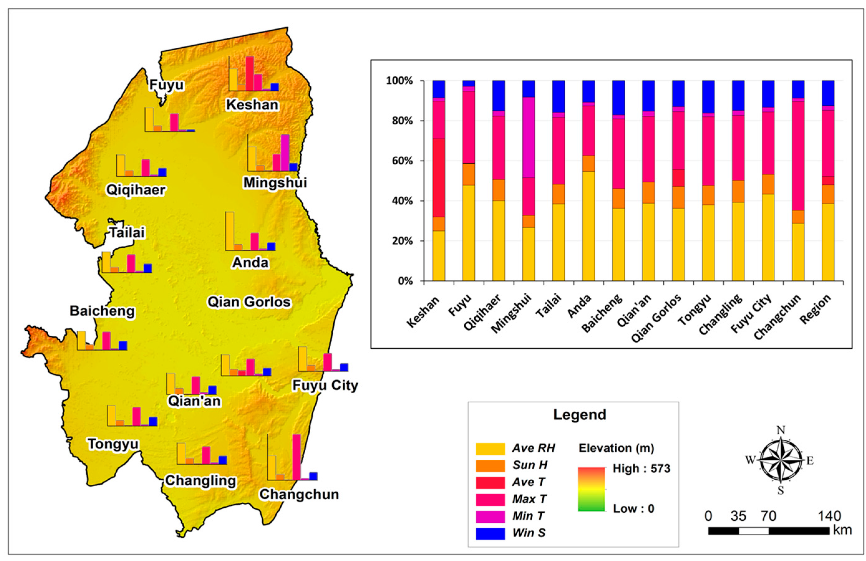
3.4. Changes in the Climatic Parameters
3.5. Sensitivity Analysis of Climatic Variables
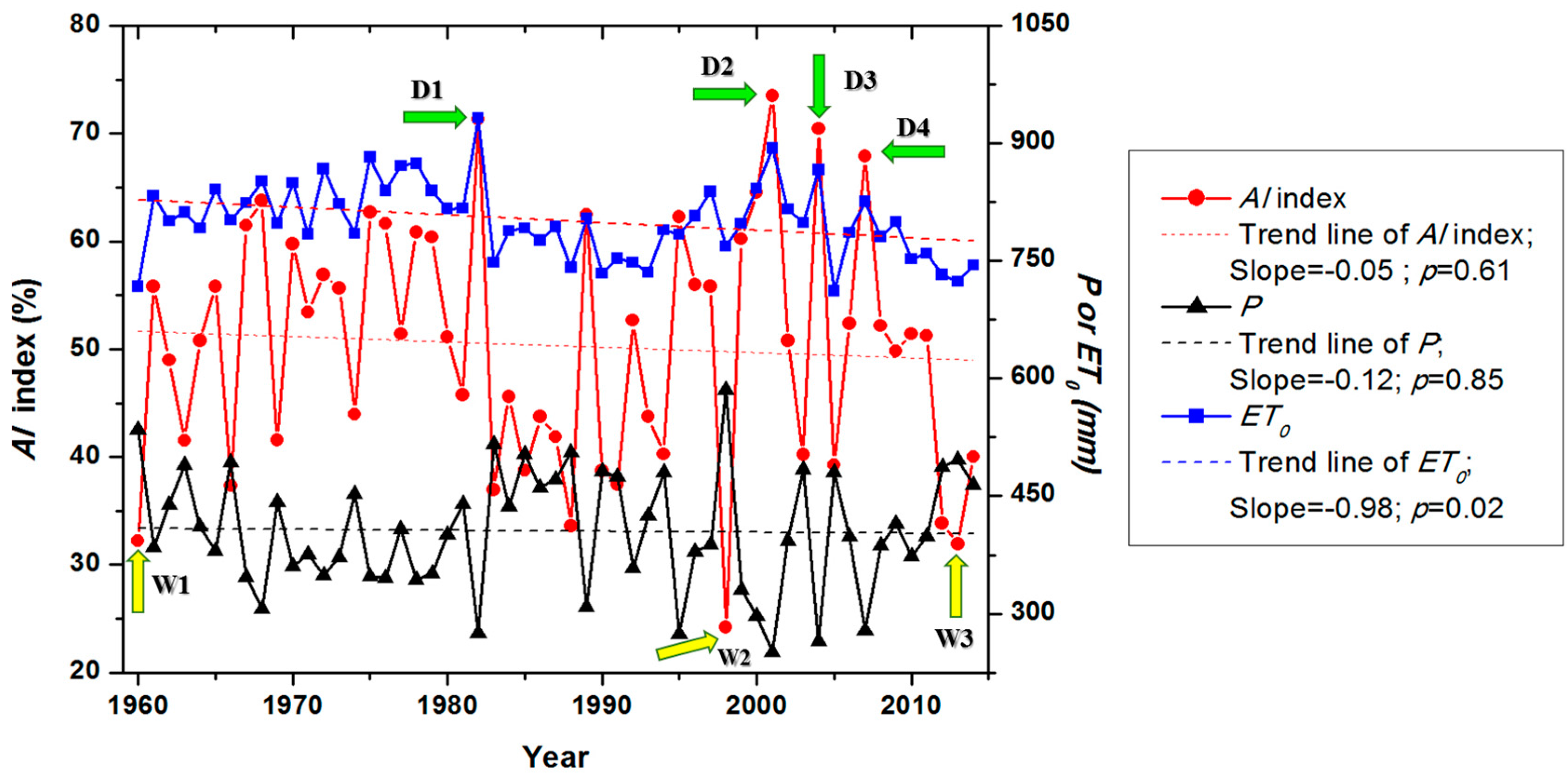
3.6. The Role of ET0 in Regional Dry/Wet Conditions
4. Discussion
5. Conclusions
- (1)
- The trend analysis of ET0 at different time scales shows an evident decreasing trend over the last 55 years, especially in the annual and spring periods. A break trend analysis shows that almost all considered climatological normal periods had experienced the decreasing trend, with a range of −2.415 to −0.003 mm per year. Abrupt changes were mainly detected in the early and mid-1990s in the annual, seasonal, and the growing season time series of ET0.
- (2)
- The spatial distributions of ET0 increased from the northeast to southwest in the annual, seasonal, and the growing season time series during 1960–2014. The spatial variations of ET0 indicated that the most significant decreasing trends were distributed in the eastern, northeastern, and central regions during the annual, spring, and growing season periods.
- (3)
- The interannual variability of climatic parameters indicated that the annual Max T, Ave T, and Min T displayed significant increasing trends at the 0.05 level (one-sided t-test), and significant decreasing trends were found for Ave RH, Win S, and Sun H. Ave RH was the dominant climate variable for the declining annual ET0 over the entire region, with the sensitivity decreasing from Max T, Win S, Sun H, Min T, to Ave T. Abrupt changes were detected in the annual time series of these variable; Ave RH in 1993, Max T in 1989, Win S in 1990, Sun H in 1987, Min T in 1983, and Ave T in 1987.
- (4)
- In general, the results of this study indicate that the regional drought/wetness condition became mildly wetter with decreasing ET0 during the growing season in the last 55 years. Regional climate drought has been alleviated in recent decades. These findings can serve as a reference for policy-makers for better planning and efficient use of agricultural water resources in the Songnen Grassland.
Acknowledgments
Author Contributions
Conflicts of Interest
References
- Stephens, G.L.; Hu, Y.X. Are climate-related changes to the character of global-mean precipitation predictable? Environ. Res. Lett. 2010, 5, 025209. [Google Scholar] [CrossRef]
- Escribano Frances, G.; Quevauviller, P.; San Martin Gonzalez, E.; Vargas Amelin, E. Climate change policy and water resources in the EU and Spain. A closer look into the Water Framework Directive. Environ. Sci. Policy 2017, 69, 1–12. [Google Scholar] [CrossRef]
- Croitoru, A.; Piticar, A.; Dragotă, C.S.; Burada, D.C. Recent changes in reference evapotranspiration in Romania. Glob. Planet. Chang. 2013, 111, 127–136. [Google Scholar] [CrossRef]
- Huo, Z.; Dai, X.; Feng, S.; Kang, S.; Huang, G. Effect of climate change on reference evapotranspiration and aridity index in arid region of China. J. Hydrol. 2013, 492, 24–34. [Google Scholar] [CrossRef]
- Fan, Z.; Thomas, A. Spatiotemporal variability of reference evapotranspiration and its contributing climatic factors in Yunnan Province, SW China, 1961–2004. Clim. Chang. 2013, 116, 309–325. [Google Scholar] [CrossRef]
- Lu, J.; Zhang, G.; Wu, F. Web-based Multi-Criteria Group Decision Support System with Linguistic Term Processing Function. IEEE Intell. Inform. Bull. 2005, 5, 35–43. [Google Scholar]
- Naderpour, M.; Lu, J.; Zhang, G. An intelligent situation awareness support system for safety-critical environments. Decis. Support Syst. 2014, 59, 325–340. [Google Scholar] [CrossRef]
- Shadmani, M.; Marofi, S.; Roknian, M. Trend Analysis in Reference Evapotranspiration Using Mann-Kendall and Spearman’s Rho Tests in Arid Regions of Iran. Water Resour. Manag. 2012, 26, 211–224. [Google Scholar] [CrossRef]
- Tabari, H.; Aghajanloo, M.B. Temporal pattern of aridity index in Iran with considering precipitation and evapotranspiration trends. Int. J. Clim. 2013, 33, 396–409. [Google Scholar] [CrossRef]
- Wang, Y.; Jiang, T.; Bothe, O.; Fraedrich, K. Changes of pan evaporation and reference evapotranspiration in the Yangtze River basin. Theor. Appl. Climatol. 2007, 90, 13–23. [Google Scholar] [CrossRef]
- Irmak, S.; Kabenge, I.; Skaggs, K.E.; Mutiibwa, D. Trend and magnitude of changes in climate variables and reference evapotranspiration over 116-yr period in the Platte River Basin, central Nebraska–USA. J. Hydrol. 2012, 420–421, 228–244. [Google Scholar] [CrossRef]
- Roderick, M.L.; Farquhar, G.D. Changes in New Zealand pan evaporation since the 1970s. Int. J. Climatol. 2005, 25, 2031–2039. [Google Scholar] [CrossRef]
- Bandyopadhyay, A.; Bhadra, A.; Raghuwanshi, N.S.; Singh, R. Temporal trends in estimates of reference evapotranspiration over India. J. Hydrol. Eng. 2009, 14, 508–515. [Google Scholar] [CrossRef]
- Liu, T.; Li, L.; Lai, J.; Liu, C.; Zhuang, W. Reference evapotranspiration change and its sensitivity to climate variables in southwest China. Theor. Appl. Climatol. 2016, 125, 1–10. [Google Scholar] [CrossRef]
- Dinpashoh, Y.; Jhajharia, D.; Fakheri-Fard, A.; Singh, V.P.; Kahya, E. Trends in reference crop evapotranspiration over Iran. J. Hydrol. 2011, 375, 65–77. [Google Scholar] [CrossRef]
- Liu, Y.; Zhuang, Q.; Pan, Z.; Miralles, D.; Tchebakova, N.; Kicklighter, D.; Chen, J.; Sirin, A.; He, Y.; Zhou, G.; et al. Response of evapotranspiration and water availability to the changing climate in Northern Eurasia. Clim. Chang. 2014, 126, 413–427. [Google Scholar] [CrossRef]
- Zheng, S.; Qin, Z.; Zhang, W. Drought variation in Songnen Plain and its response to climate change. Chin. J. Agrometeorol. 2015, 36, 640–649. [Google Scholar]
- Zhang, Y.; Deng, J.; Guan, D.; Jin, C.; Wang, A.; Wu, J.; Yuan, F. Spatiotemporal changes of potential evapotranspiration in Songnen Plain of Northeast China. Chin. J. Appl. Ecol. 2011, 22, 1702–1710. [Google Scholar]
- Limin, S.G.; Oue, H.; Takase, K. Estimation of areal average rainfall in the mountainous Kamo River Watershed, Japan. J. Agric. Meteorol. 2015, 71, 90–97. [Google Scholar] [CrossRef]
- Allen, R.G.; Pereira, L.S.; Raes, D.; Smith, M. Crop Evapotranspiration-Guidelines for Computing Crop Water Requirements—FAO Irrigation and Drainage; FAO: Rome, Italy, 1998; p. 56. [Google Scholar]
- Mosaedi, A.; Sough, M.G.; Sadeghi, S.; Mooshakhian, Y.; Bannayan, M. Sensitivity analysis of monthly reference crop evapotranspiration trends in Iran: A qualitative approach. Theor. Appl. Climatol. 2017, 128, 857–873. [Google Scholar] [CrossRef]
- Liu, C.; Zhang, D.; Liu, X.; Zhao, C. Spatial and temporal change in the potential evapotranspiration sensitivity to meteorological factors in China (1960–2007). J. Geogr. Sci. 2012, 22, 3–14. [Google Scholar] [CrossRef]
- Kendall, M.G. Rank Correlation Methods; Griffin: London, UK, 1948. [Google Scholar]
- Mann, H.B. Nonparametric tests against trend. Econometrica 1945, 13, 245–259. [Google Scholar] [CrossRef]
- Wang, W.; Zhu, Y.; Xu, R.; Liu, J. Drought severity change in China during 1961–2012 indicated by SPI and SPEI. Nat. Hazards 2015, 75, 2437–2451. [Google Scholar] [CrossRef]
- Zhang, Q.; Zhang, J. Drought hazard assessment in typical corn cultivated areas of China at present and potential climate change. Nat. Hazards 2016, 81, 1323–1331. [Google Scholar] [CrossRef]
- Yan, T.; Shen, Z.; Bai, J. Spatial and temporal changes in temperature, precipitation, and streamflow in the Miyun Reservoir Basin of China. Water 2017, 9, 78. [Google Scholar] [CrossRef]
- Tabari, H.; Taye, M.T.; Willems, P. Statistical assessment of precipitation trends in the upper Blue Nile River basin. Stoch. Environ. Res. Risk Assess. 2015, 29, 1751–1961. [Google Scholar] [CrossRef]
- Palizdan, N.; Falamarzi, Y.; Huang, Y.F.; Lee, T.S. Precipitation trend analysis using discrete wavelet transform at the Langat River Basin, Selangor, Malaysia. Stoch. Environ. Res. Risk Assess. 2017, 31, 853–877. [Google Scholar] [CrossRef]
- Liang, L.; Li, L.; Liu, Q. Temporal variation of reference evapotranspiration during 1961–2005 in the Taoer River basin of Northeast China. Agric. For. Meteorol. 2010, 150, 298–306. [Google Scholar] [CrossRef]
- Sen, P.K. Estimates of the regression coefficient based on Kendall’s tau. J. Am. Stat. Assoc. 1968, 63, 1379–1389. [Google Scholar] [CrossRef]
- Salmi, T.; Maatta, A.; Anttila, P.; Ruoho-Airola, T.; Amnell, T. Detecting Trends of Annual Values of Atmospheric Pollutants by the Mann-Kendall Test and Sen’s Slope Estimates—The Excel Template Application MAKESENS; Publications on Air Quality 31; Report Code FMIAQ-31; Universitas Gadjah Mada: Yogyakarta, The Republic of Indonesia, 2002. [Google Scholar]
- Madhu, S.; Kumar, T.V.L.; Barbosa, H.; Rao, K.K.; Bhaskar, V.V. Trend analysis of evapotranspiration and its response to droughts over India. Theor. Appl. Climatol. 2015, 121, 41–51. [Google Scholar] [CrossRef]
- Arguez, A.; Vose, R.S. The Definition of the Standard WMO Climate Normal: The Key to Deriving Alternative Climate Normals. Bull. Am. Meteorol. Soc. 2011, 92, 699–704. [Google Scholar] [CrossRef]
- Zhao, L.; Xia, J.; Sobkowiak, L.; Li, Z. Climatic characteristics of reference evapotranspiration in the Hai River Basin and their attribution. Water 2014, 6, 1482–1499. [Google Scholar] [CrossRef]
- Zheng, C.; Wang, Q. Spatiotemporal pattern of the global sensitivity of the reference evapotranspiration to climatic variables in recent five decades over China. Stoch. Environ. Res. Risk. Assess. 2015, 29, 1937–1947. [Google Scholar] [CrossRef]
- Zhan, X.; Kustas, W.P.; Humes, K.S. An intercomparison study on models of sensible heat flux over partial canopy surfaces with remotely sensed surface temperature. Remote Sens. Environ. 1996, 58, 242–256. [Google Scholar] [CrossRef]
- Su, X.; Singh, V.P.; Niu, J.; Hao, L. Spatiotemporal trends of aridity index in Shiyang River basin of northwest China. Stoch. Environ. Res. Risk. Assess. 2015, 29, 1571–1582. [Google Scholar] [CrossRef]
- Thornthwaite, C.W. An approach toward a rational classification of climate. Geogr. Rev. 1948, 38, 55–89. [Google Scholar] [CrossRef]
- Zhang, K.; Pan, S.; Zhang, W.; Xu, Y.; Cao, L.; Hao, Y.; Wang, Y. Influence of climate change on reference evapotranspiration and aridity index and their temporal-spatial variations in the Yellow River Basin, China, from 1961 to 2012. Quat. Int. 2015, 380–381, 75–82. [Google Scholar] [CrossRef]
- Ashraf, M.; Routray, J.K. Spatio-temporal characteristics of precipitation and drought in Balochistan Province, Pakistan. Nat. Hazards 2015, 77, 229–254. [Google Scholar] [CrossRef]
- Li, X.; Gemmer, M.; Zhai, J.; Liu, X.; Su, B.; Wang, Y. Spatio-temporal variation of actual evapotranspiration in the Haihe River Basin of the past 50 years. Quat. Int. 2013, 304, 133–141. [Google Scholar] [CrossRef]
- Piticar, A.; Mihăilă, D.; Lazurca, L.G.; Bistricean, P.; Puţuntică, A.; Briciu, A. Spatiotemporal distribution of reference evapotranspiration in the Republic of Moldova. Theor. Appl. Climatol. 2016, 124, 1133–1144. [Google Scholar] [CrossRef]
- Yin, Y.; Wu, S.; Chen, G.; Dai, E. Attribution analyses of potential evapotranspiration changes in China since the 1960s. Theor. Appl. Climatol. 2010, 101, 19–28. [Google Scholar] [CrossRef]
- Dong, B.; Sutton, R.T.; Chen, W.; Liu, X.; Lu, R.; Sun, Y. Abrupt summer warming and changes in temperature extremes over Northeast Asia since the mid-1990s: Drivers and physical processes. Adv. Atmos. Sci. 2016, 33, 1005–1023. [Google Scholar] [CrossRef]
- Liu, S.; Yang, S.; Lian, Y.; Zheng, D.; Wen, M.; Tu, G.; Shen, B.; Gao, Z.; Wang, D. Time–frequency characteristics of regional climate over northeast China and their relationships with atmospheric circulation patterns. J. Clim. 2010, 23, 4956–4972. [Google Scholar] [CrossRef]
- Gong, D.Y.; Wang, S.W. Influence of Arctic Oscillation on Winter Climate over China. J. Geogr. Sci. 2003, 13, 208–216. [Google Scholar]
- Li, J.; Jiao, M.; Hu, C.; Li, F.; Zhang, X.; Zhang, Q.; Wang, Y.; Zhu, X. Characteristics of summer temperature and its impact factors in Northeast China from 1951 to 2012. J. Meteorol. Environ. 2016, 32, 74–83. [Google Scholar]
- Espadafor, M.; Lorite, I.J.; Gavilan, P.; Berengena, J. An analysis of the tendency of reference evapotranspiration estimates and other climate variables during the last 45 years in Southern Spain. Agric. Water Manag. 2011, 98, 1045–1061. [Google Scholar] [CrossRef]


 indicates the detected change point.
indicates the detected change point.
indicates the detected change point.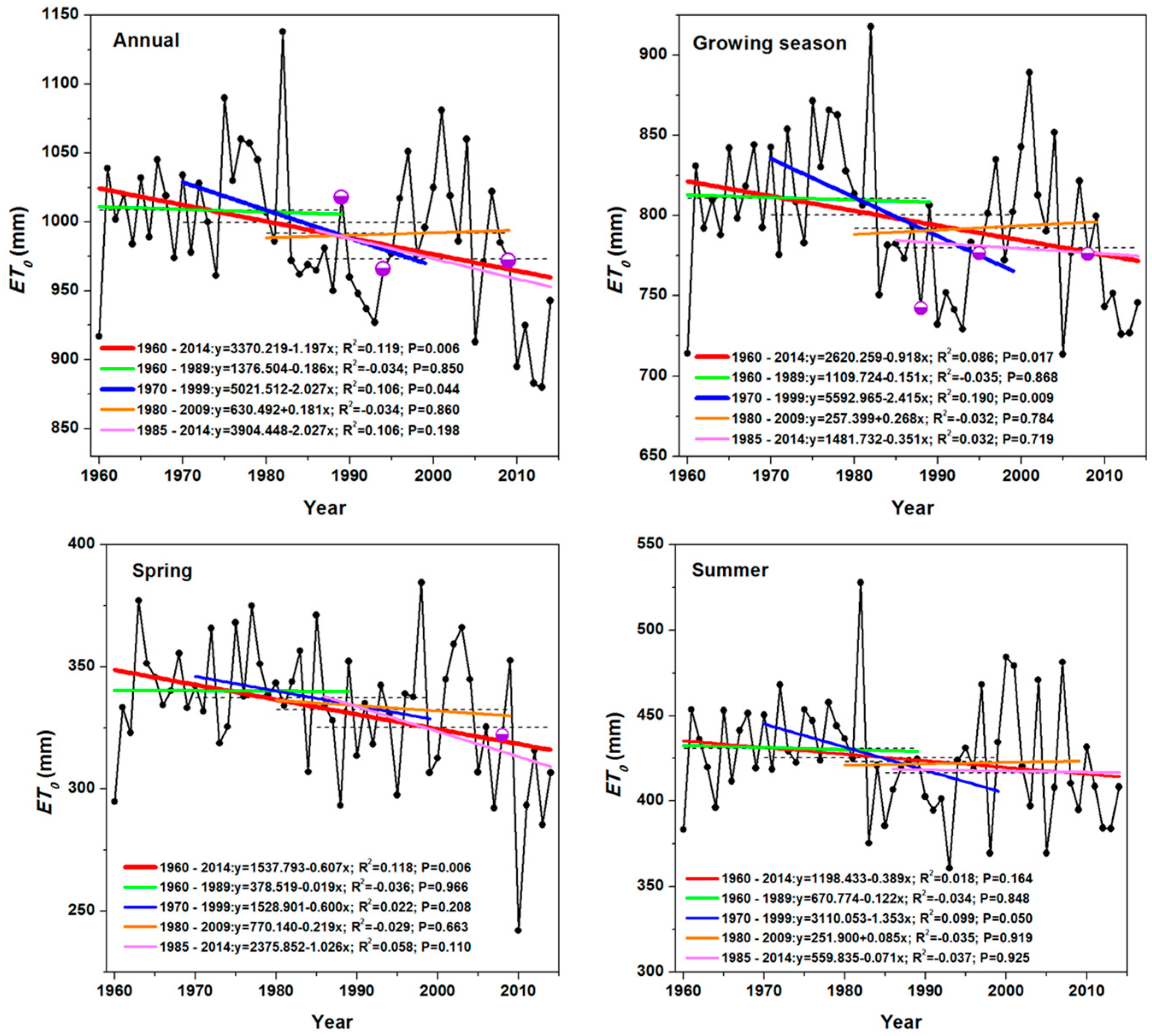

 indicates the detected change point.
indicates the detected change point.
indicates the detected change point.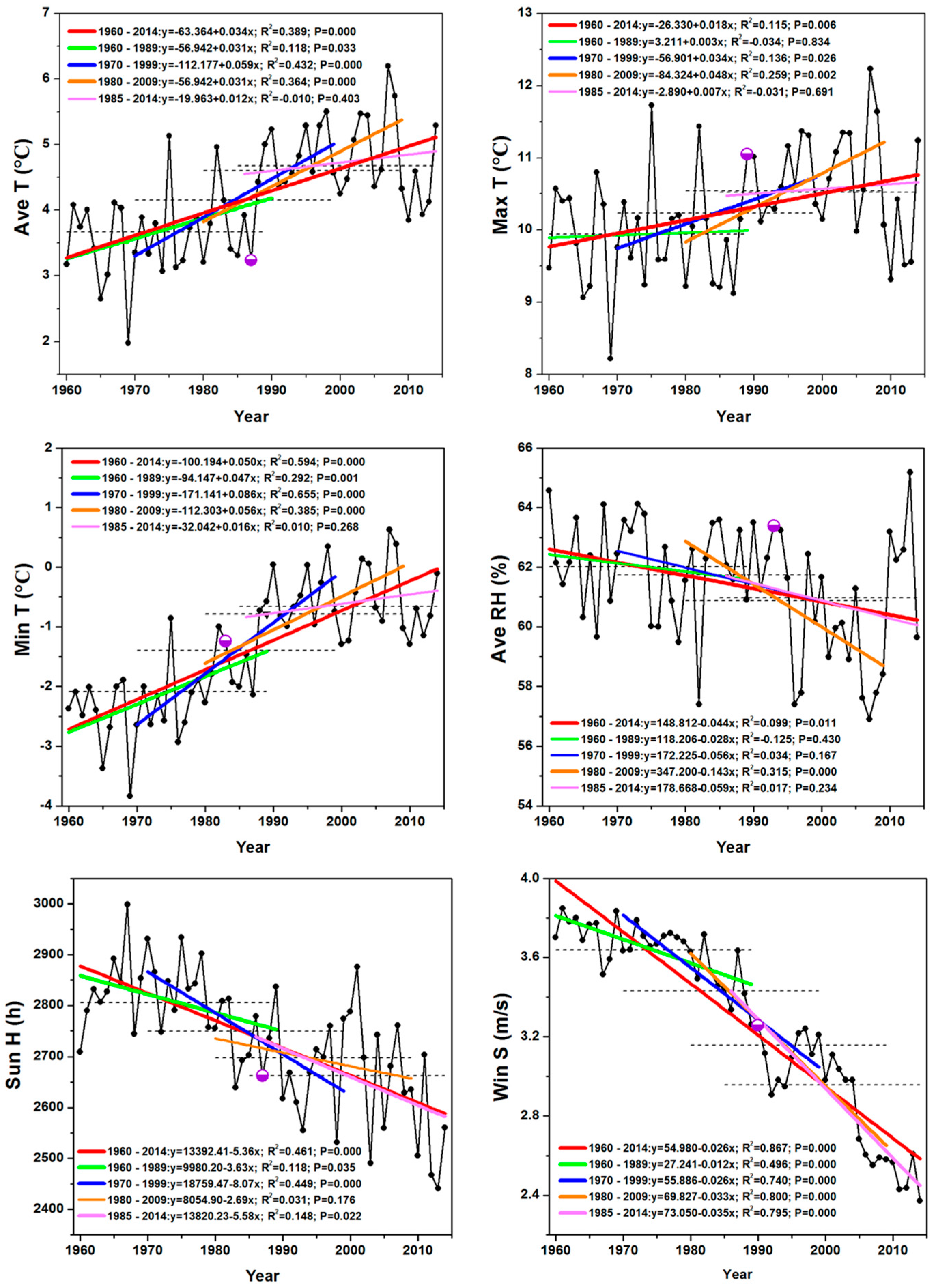


| Station | Order and Trend of the Sensitivity for the Climatic Variables in ET0 | |||||||||||
|---|---|---|---|---|---|---|---|---|---|---|---|---|
| Keshan | Ave T | −5.55 * | Ave RH | −3.54 * | Max T | −3.59 * | Win S | −0.81 | Sun H | 3.85 * | Min T | 0.94 |
| Fuyu | Ave RH | −2.38 * | Max T | −3.17 * | Sun H | 2.06 * | Min T | 1.56 | Win S | 0.07 | Ave T | 1.10 |
| Qiqihaer | Ave RH | −4.56 * | Max T | −4.15 * | Win S | 1.31 | Sun H | 2.06 * | Min T | 4.24 * | Ave T | 0.00 |
| Mingshui | Min T | −6.90 * | Ave RH | −3.96 * | Max T | −4.85 * | Win S | 0.64 | Sun H | 1.51 | Ave T | 0.00 |
| Tailai | Ave RH | −3.89 * | Max T | −3.12 * | Win S | 4.02 * | Sun H | 1.29 | Min T | 3.66 * | Ave T | 0.00 |
| Anda | Ave RH | 2.83 * | Max T | −3.56 * | Win S | 0.20 | Sun H | 4.07 * | Min T | 0.40 | Ave T | 0.00 |
| Baicheng | Ave RH | −3.05 * | Max T | −3.03 * | Win S | 1.19 | Sun H | 1.80 | Min T | 2.08 * | Ave T | 0.00 |
| Qian’an | Ave RH | −2.90 * | Max T | −2.87 * | Win S | 2.53 * | Sun H | 0.28 | Min T | 1.68 | Ave T | 0.00 |
| Qian Gorlos | Ave RH | −6.27 * | Max T | −4.66 * | Win S | 0.96 | Sun H | 3.53* | Ave T | −4.72 * | Min T | 2.31 * |
| Tongyu | Ave RH | −2.95 * | Max T | −1.74 | Win S | 3.03 * | Sun H | −0.15 | Min T | 1.06 | Ave T | 0.00 |
| Changling | Ave RH | −3.27 * | Max T | −2.63 * | Win S | 4.01 * | Sun H | −1.26 | Min T | 2.42 * | Ave T | 0.00 |
| Fuyu City | Ave RH | −5.62 * | Max T | −4.37 * | Win S | 2.42 * | Sun H | 1.28 | Min T | 3.14 * | Ave T | 0.00 |
| Changchun | Max T | 3.11 * | Ave RH | −6.11 * | Win S | 1.97 * | Sun H | 3.47 * | Min T | 2.24 * | Ave T | 0.00 |
| Region | Ave RH | −4.07 * | Max T | −4.18 * | Win S | 2.90 * | Sun H | 3.92 * | Ave T | −6.94 * | Min T | −7.93 * |
© 2017 by the authors. Licensee MDPI, Basel, Switzerland. This article is an open access article distributed under the terms and conditions of the Creative Commons Attribution (CC BY) license (http://creativecommons.org/licenses/by/4.0/).
Share and Cite
Ma, Q.; Zhang, J.; Sun, C.; Guo, E.; Zhang, F.; Wang, M. Changes of Reference Evapotranspiration and Its Relationship to Dry/Wet Conditions Based on the Aridity Index in the Songnen Grassland, Northeast China. Water 2017, 9, 316. https://doi.org/10.3390/w9050316
Ma Q, Zhang J, Sun C, Guo E, Zhang F, Wang M. Changes of Reference Evapotranspiration and Its Relationship to Dry/Wet Conditions Based on the Aridity Index in the Songnen Grassland, Northeast China. Water. 2017; 9(5):316. https://doi.org/10.3390/w9050316
Chicago/Turabian StyleMa, Qiyun, Jiquan Zhang, Caiyun Sun, Enliang Guo, Feng Zhang, and Mengmeng Wang. 2017. "Changes of Reference Evapotranspiration and Its Relationship to Dry/Wet Conditions Based on the Aridity Index in the Songnen Grassland, Northeast China" Water 9, no. 5: 316. https://doi.org/10.3390/w9050316
APA StyleMa, Q., Zhang, J., Sun, C., Guo, E., Zhang, F., & Wang, M. (2017). Changes of Reference Evapotranspiration and Its Relationship to Dry/Wet Conditions Based on the Aridity Index in the Songnen Grassland, Northeast China. Water, 9(5), 316. https://doi.org/10.3390/w9050316