Abstract
Modeling insecurity under future climate change and socio-economic development is indispensable for adaptive planning and sustainable management of water resources. This case study strives to assess the water quality and quantity status for both the present and the near future in the Ciliwung River basin inside the Jakarta Province under different scenarios using population growth with planned additional wastewater management infrastructure by 2030 as mentioned in the local master plan, and comparing the above conditions with the addition of the effects of climate change. Biochemical oxygen demand (BOD), chemical oxygen demand (COD) and nitrate (NO3), the three important indicators of aquatic ecosystem health, were simulated to assess river pollution. Simulation results suggest that water quality in year 2030 will further deteriorate compared to the base year 2000 due to population growth and climate change, even considering the planned wastewater management infrastructure. The magnitude of impact from population growth is far greater than that from climate change. Simulated values of NO3, BOD and COD ranged from 6.07 to 13.34 mg/L, 7.65 to 11.41 mg/L, and 20.16 to 51.01 mg/L, respectively. Almost all of the water quality parameters exceeded the safe limit suitable for a healthy aquatic system, especially for the year 2030. The situation of water quality is worse for the downstream sampling location because of the cumulative effect of transport of untreated pollutants coming from upstream, as well as local dumping. This result will be useful for local policy makers and stakeholders involved in the water sector to formulate strategic and adaptive policies and plan for the future. One of the potential policy interventions is to implement a national integrated sewerage and septage management program on a priority basis, considering various factors like population density and growth, and global changes for both short- and long-term measures.
1. Introduction and Research Background
Globally, it is estimated that nearly two-thirds of all nations will experience water stress by the year 2025 [1]. The main problem may not be scarcity of water in terms of average per capita but the high cost of making water available at the right place, at the right time and with the required quality. Therefore, ensuring good quality water availability and sustainable management of water for all by the year 2030 is one of the top priorities of the United Nations Sustainable Development Goals (SDGs) [2]. Intense agricultural and industrial activities in any area are likely to make water resources vulnerable with respect to their quality and quantity [3,4]. The fragile institutional capability of the concerned agencies involved in the water policies sector in developing countries makes the conditions worse, and henceforth there is a continual decline of the water quality of freshwater resources at a global scale [5]. From a human use perspective, this generally results in increasing costs associated with water treatment and a decline in the availability of usable water [6]. While increasing population and economic development are also blamed for increasing pollution of freshwater resources, it is likely that future climate change will exacerbate water quality problems [7]. Therefore, the development of management and adaptive measures for managing water quality should collectively take future developmental and climate change effects into account [8,9]. Doubts over data, models and impacts of economic and social factors all contribute to increasing the uncertainty associated with the results of modeled future scenarios [10]. Therefore, uncertainty needs to be incorporated into water resource planning to facilitate adaptive planning [11,12,13]. The formulation of water quality management strategies requires the inter-disciplinary analysis of various potential causes of water quality degradation and corresponding solutions [14,15]. Mathematical models are widely used to simulate the pollution of water bodies for likely wastewater production and treatment scenarios [16,17,18]. These models may be based on physical data or a simplified conceptual or empirical approach. In the case of countries with limited financial resources, for any water quality model to be useful, it should not be data-intensive or too complex to operate. Selection of a water quality model depends on data availability, calculation time, and intended output variables with a policy-setting interface. The Water Evaluation and Planning (WEAP) model, a decision support system of the Stockholm Environmental Institute, is widely used for water quality simulation based on different scenario formulations and is ultimately used for integrated water resource planning and management [19,20,21,22].
Recently, the situation of water security in the most populous and rapidly developing regions, especially the megacities of Asia, is worsening because of major challenges such as overexploitation of groundwater, skewed water supply and demand due to population explosion and the negative impacts of climate change [23]. In Southeast Asia, the archipelago of Indonesia is the wealthiest nation in terms of water resources, which has played an important role in the rapid development of Indonesia over the past decades. Even though plenty of water resources are available, the cumulative effects of the tropical climate, topography, general environment and increasing user demands (e.g., irrigation, industries, and domestic) impose greater challenges on their management in the current situation [24]. Together with these challenges, protection from floods has been at the heart of the public works administration over the past centuries [25]. Jakarta, which is the Indonesian capital, also serves as the most important economic, political and cultural hub of the country. With uncoordinated brisk urban expansion, inadequate wastewater treatment facilities, low levels of awareness and fragile institutional capability of the concerned agencies, huge amounts of wastewater are generated that cause deterioration of the surface water resources. In Jakarta, clean water use is 413 million m3 a year, but the supply from the District Water Utility reservoirs is limited to 200 million m3, which indicates that the rest of the 213 million m3 of clean water needed by Jakarta is dependent on underground water reservoirs [26]. The other problem is with respect to the rapid change in land development (from vegetation to built-up areas) around the Ciliwung River basin area over the last three decades. This results in ecosystem degradation and ultimately leads to a decrease in land fertility, water quality deterioration, drought during the dry season, and floods during the wet season. So far, very few studies have addressed the status of water resources and their management strategies in the near future.
This work intends to assess the current situation (year 2015) and simulated future outlook (year 2030) with regard to water demand and quality deterioration using key indicators, which are biochemical oxygen demand (BOD), chemical oxygen demand (COD) and nitrate (NO3), under two different scenarios in the Ciliwung River, and is ultimately aimed at helping formulate sustainable water resource management options.
2. Study Area
The area of interest for this research is downstream of the Ciliwung River basin, intersecting the Special Capital City District of Jakarta (DKI Jakarta) including the entire watershed area of approximately 420 km2 (Figure 1). The Ciliwung River basin starts upstream at Tugu Puncak, Bogor Province and flows northward through the cities of Depok and Jakarta and finally ends at Jakarta Bay. Of the 117 km of the river, this study focuses on a 75-km length of the Ciliwung River inside Jakarta City with an elevation ranging from 5 to 350 m above mean sea level (MAMSL) that supports approximately 4.5 million people. Jakarta, which is officially known as the Special Capital Region of Jakarta, is the economic, political and cultural capital of Indonesia. The average annual rainfall is approximately 2683 mm. The mean annual temperature is approximately 29 °C. Based on the land use/land cover map, the entire area is divided into the following classes: building, farmland, forests, freshwater, grass, open land, paddy field, river, swamp, tree, and urban areas. Rapid urbanization and exponential population growth in Jakarta and the nearby megacity area, called Jabodetabek (Jakarta-Bogor-Depok-Tanggerang-Bekasi), have resulted in environmental deterioration, especially of water resources.
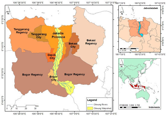
Figure 1.
Location of the Ciliwung River basin.
3. Methods
3.1. Basic Information Regarding the Model and Data Requirements
The Water Evaluation and Planning (WEAP) model greatly supports scenario formation functionalities where policy alternatives can be considered for current and future conditions. The WEAP hydrology module enables estimation of rainfall-runoff and pollutant travel from a catchment to water bodies [20]. Scenarios are developed based on population growth, industrial and commercial activities, land use/land cover, the capacity and status of treatment plants, climate change, and several other factors that can significantly impact wastewater levels. WEAP provides a Geographical Information System (GIS)-based interface to graphically represent wastewater generation and treatment systems. A variety of applications of WEAP for water quality modeling and ecosystem preservation have been reported [21,22,27]. WEAP can simulate several conservative water quality variables (which follow exponential decays) and non-conservative water quality variables in addition to pollution generation and removal at different sites.
The WEAP model was used to simulate future total water demand and water quality variables in the year 2030 to assess alternative management policies in the Ciliwung River basin. Apart from our main objective, it also simulates river flow, storage, pollution generation, treatment and discharge, while considering different users and environmental flows.
For water quality modeling, a wide range of input data including point and non-point pollution sources, their locations and concentrations, past spatio-temporal water quality, wastewater treatment plants (Ministry of Public Works), population, historical rainfall, evaporation, temperatures (Indonesian Agency for Meteorology, Climatology and Geophysics), drainage networks (Department of Public Works), river flow-stage-width relationships, river length, groundwater, surface water inflows and land use/land cover (Indonesian Institute of Sciences (LIPI)) is provided.
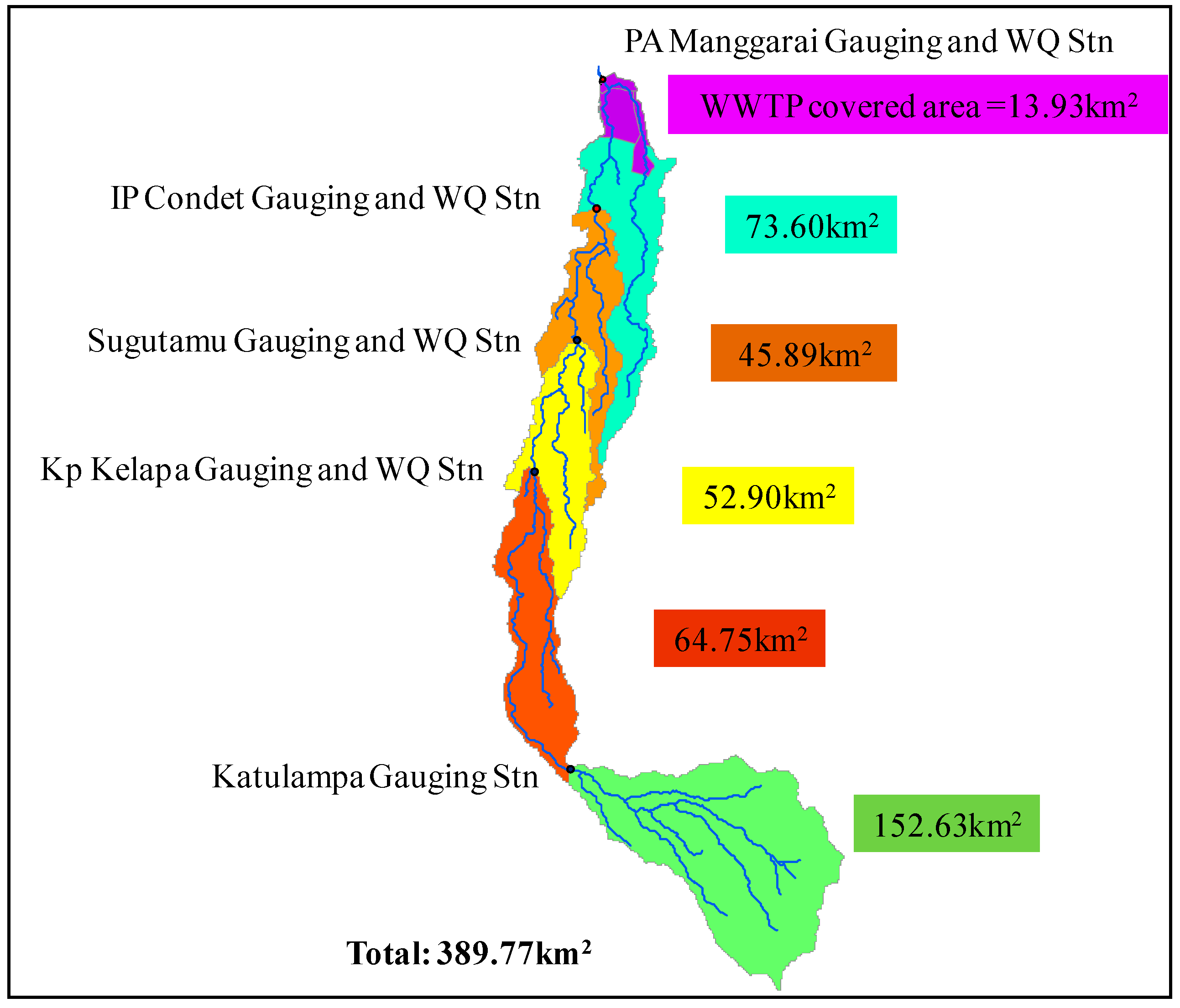
The WEAP model was developed for the Ciliwung River basin for four command areas with inter-basin transfers. Hydrologic modeling requires the entire study area to be split into smaller catchments with consideration of the confluence points and physiographic and climatic characteristics (Figure 2). The hydrology module within the WEAP tool enables modeling of the catchment runoff and pollutant transport processes into the river. Pollutant transport from a catchment accompanied by rainfall-runoff is enabled by ticking the water quality modeling option. Pollutants that accumulate on catchment surfaces during non-rainy days reach water bodies through surface runoff. The WEAP hydrology module computes catchment surface pollutants generated over time by multiplying the runoff volume and concentration or intensity for different types of land use.
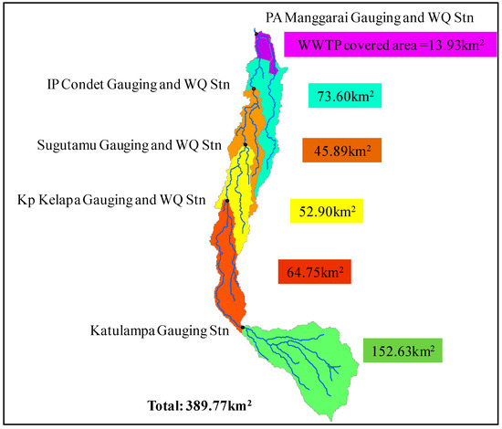
Figure 2.
The Ciliwung River network with sub-catchments and locations of wastewater treatment plants, water quality stations, and streamflow measurement stations. WWTP: wastewater treatment plant. (Here- WQ Stn—Water Quality Station).
During simulation, the land use information was broadly categorized into three categories, viz., agricultural, forest, and built-up areas. The soil data parameters were identified using previous secondary data and the literature [25].
Different hydroclimatic data, such as daily rainfall, air temperature, relative humidity and wind velocity, were used and had been collected at meteorological stations, namely, Citeko, Darmaga, Kemayoran and Tanjung Priok, for the period from 1980 to 2016. Daily average stream flow data from 1984 to 2016 were measured at five stations, namely, Katulampa, Kelapa, Sugutamu, IP Condet and Manggarai of the Ciliwung River, and were utilized to calibrate and validate the WEAP hydrology module simulation. Data for the water quality indicators (BOD, COD and NO3) were also collected at four of the above five stations and used for water quality modeling (Figure 2).
Data for the population distribution and its future trend at these five small command areas were provided by the Indonesian Institute of Sciences (LIPI) using a cohort component analysis method. Here, data for 2015 and 2030 are used for simulation in the reference and future scenarios, respectively (Table 1).

Table 1.
The yearly trend for population distribution in different command areas of the study area.
Regarding future climatic variables, the general circulation model (GCM) output is downscaled at the local level for reliable impact assessment [28,29,30,31]. Statistical downscaling followed by quantile-based bias correction, a less computation-demanding technique which enables reduction of biases in the precipitation frequency and intensity [32], is used here to get climate variables with a temporal resolution of 3 h and a spatial resolution of 120 km. This temporal resolution is well-suited to our observed precipitation data on a daily basis. The MRI-CGCM3.2 (Meteorological Research Institute, Japan) precipitation output at the Katulampa Gauging station was used for the future simulation to assess the climate change impact because of its wide use and high temporal resolution compared to other climate models. This study is based on the Representative Concentration Pathway (RCP) 4.5 emission scenario, which assumes that global annual Green House Gas (GHG) emissions (measured in CO2-equivalents) peak around 2040 and then decline [33]. In this study, the GCM data are from 1985 to 2004 and from 2020 to 2039 (both 20-year periods) and represent the current and future (2030) climate, respectively. In this technique, simulated deviations in the daily frequency distribution of GCM precipitation are applied to observed precipitation [32]. For the bias correction, precipitation frequency of scanty precipitation days to dry days is altered such that number of GCM and observation wet days are approximately identical. In this study, empirical frequency analysis was carried out to estimate long-term probability of dry (zero precipitation values) days in the observation data series. Accordingly, a threshold (GCM precipitation value) corresponded to a non-exceedance probability of zero observations of precipitation is selected. A GCM precipitation intensity above the threshold value is corrected by taking the inverse of the cumulative distribution function (CDF) of GCM data with the observation distribution parameters. In order to correct future GCM precipitation data series, a scaling factor is derived for each of the quantiles. The scaling factor is ratio of the inverse of CDF of future GCM precipitation to the observed and present GCM precipitation datasets. Here, two-parameter gamma distribution was employed for bias correction.
3.2. Hydrologic Modeling
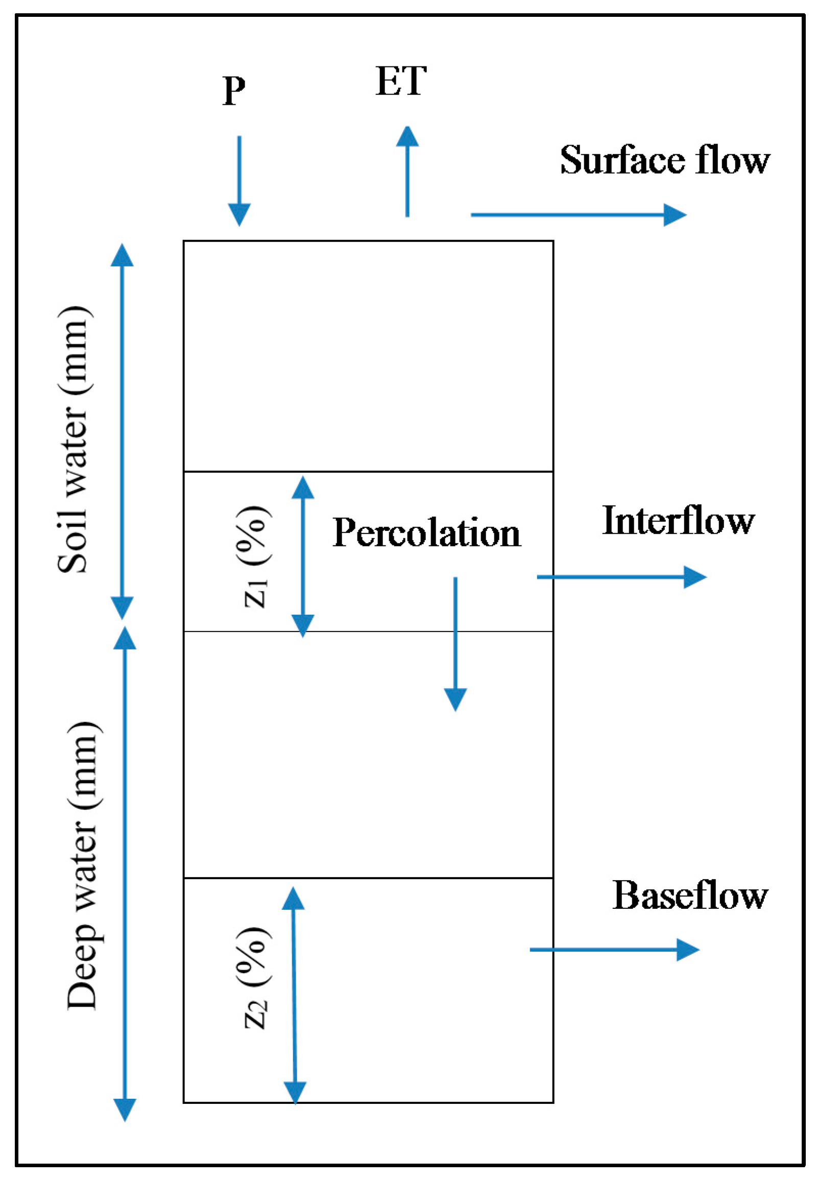
Under the WEAP hydrology module, the soil moisture method (which is the most sophisticated and widely accepted method) is used to estimate the different hydrological parameters for this study (Figure 3). This method can simulate different components of the hydrologic cycle, including evapotranspiration (ET), surface runoff, interflow, base flow, and deep percolation [19]. Empirical equations are employed to describe the rainfall-runoff and pollutant transport processes. With the soil moisture method, each catchment is split into two soil layers: an upper soil layer and a lower soil layer, which represent shallow water and deep water capacities, respectively. The upper soil layer accounts for spatial variation in different kinds of land use and soil types. The lower soil layer is meant to represent groundwater recharge and baseflow processes, and its parameters remain the same for the entire catchment. Different hydrological components are estimated, with z1 and z2 as the initial relative storage (%) for the upper (root zone) and lower (deep) water capacity, respectively (Equations (1)–(5)).
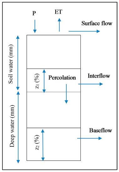
Figure 3.
Conceptual diagram of a two-bucket hydrological model. ET: evapotranspiration; z1 and z2 are upper soil layer and lower soil layer (m) respectively.
Pollutant transport from a catchment accompanied by rainfall-runoff is enabled by ticking the water quality modeling option. Pollutants that accumulate on catchment surfaces during non-rainy days reach water bodies through surface runoff. The WEAP hydrology module computes the catchment surface pollutants generated over time by multiplying the runoff volume and concentration or intensity for different types of land use [19].
z1 and z2 = upper soil layer and lower soil layer (m), which represent shallow water and deep water capacities, respectively.
3.3. Stream Water Quality Modeling
The water quality module of the WEAP tool makes it possible to estimate the pollution concentrations in water bodies and is based on the Streeter–Phelps model. In this model, the simulation of oxygen balance in a river is governed by two processes: consumption by decaying organic matter and reaeration induced by the oxygen deficit [19]. BOD removal from water is a function of the water temperature, settling velocity, and water depth (Equations (6)–(9)):
where,
- BODinit = BOD concentration at the beginning of the reach (mg/L)
- BODfinal = BOD concentration at the end of the reach (mg/L)
- t = water temperature (in °C)
- H = water depth (m)
- L = reach length (m)
- U = water velocity in the reach
- vs = settling velocity (m/s)
- kr, kd and ka = total removal, decomposition and aeration rate constants (L/time)
- kd20 = decomposition rate at the reference temperature (20 °C)
The oxygen concentration in the water is a function of the water temperature and BOD:
- Ofinal = oxygen concentration at the end of the reach (mg/L)
- Oinitial = oxygen concentration at the beginning of the reach (mg/L)
Ideally, field measurements should be conducted and analyzed to obtain values for the different parameters. However, extensive time and financial requirements restrict the use of field measurements to directly identify several water quality module parameters. Therefore, most water quality modeling parameters are estimated using the established literature and reports [34].
Similarly, simulation for chemical oxygen demand (COD) and nitrate (NO3) is conducted considering consumption by decaying organic and inorganic matter and reaeration induced by the oxygen deficit.
3.4. Model Setup
The entire problem domain and its different components are divided into five catchments, which are further subdivided into thirteen sub-basins considering influent locations of major tributaries (Figure 4). Other major considerations are the fourteen demand sites and one wastewater treatment plant to represent the problem domain. Here, demand sites are meant to identify domestic (population) and industrial centers defined with their attributes explaining water consumption and wastewater pollution loads per capita, water supply source, and wastewater return flow. Dynamic attributes are described as functions of time and include population and industries. Wastewater treatment plants (WWTPs) are pollution-handling facilities with design specifications that include total capacity and removal rates of pollutants. The flow of wastewater into the Ciliwung River and its tributaries mainly feeds through domestic, industrial and stormwater runoff routes. Here, an upflow anaerobic sludge blanket reactor (USAB) type of wastewater treatment plant is considered in the modeling and its pollutant treatment capacity is assumed accordingly. No precise data are available regarding the total volume of wastewater production from different sources. In the absence of detailed information, the daily volume of domestic wastewater generation is based on an estimated 130 L of average daily consumption per capita [1].
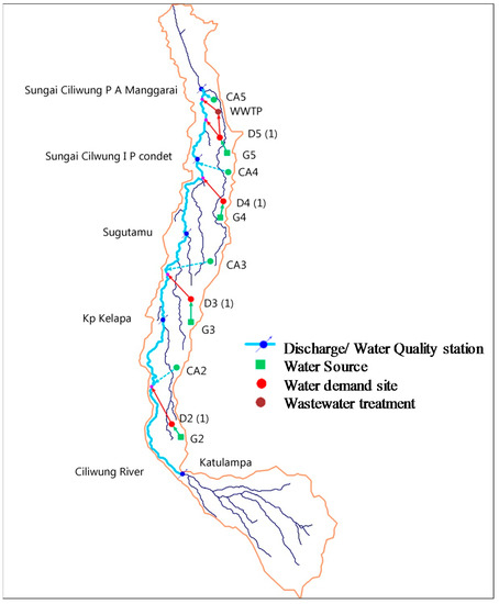
Figure 4.
A schematic diagram showing the problem domain for water quality modeling in Jakarta Province using the Water Evaluation and Planning (WEAP) interface.
The scenario analysis is conducted by defining a time horizon based on which alternative wastewater generation and management options can be explored. The business as usual condition is represented by a reference scenario with selection of all the existing elements as currently active. Consequently, the new/upgraded WWTPs (information taken from local master plan) are modeled as scenarios representing deviations from the current conditions (reference scenario). Detailed information on existing (functional) and planned wastewater treatment plants in DKI Jakarta used for modeling is mentioned in Table 2. Under current reference scenario conditions (baseline year 2000), only the Setiabudi WWTP was operational, with coverage area of mere 2% of the total population. To model future conditions, all three (one upgraded and two new proposed) WWTPs were enabled by defining respective start-up years.
Table 2.
Existing (functional) and planned wastewater treatment plants in DKI Jakarta. BOD: biochemical oxygen demand.
Information on each object can easily be retrieved by clicking the corresponding graphical element, and the baseline year under the current reference scenario in this study is 2000.
4. Results and Discussion
4.1. Model Performance Evaluation
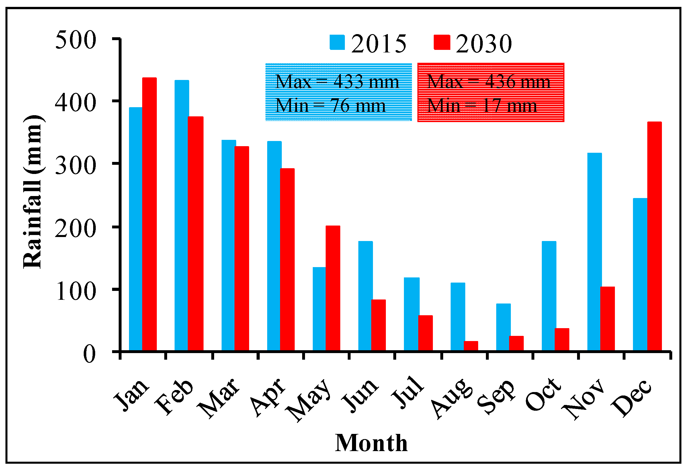
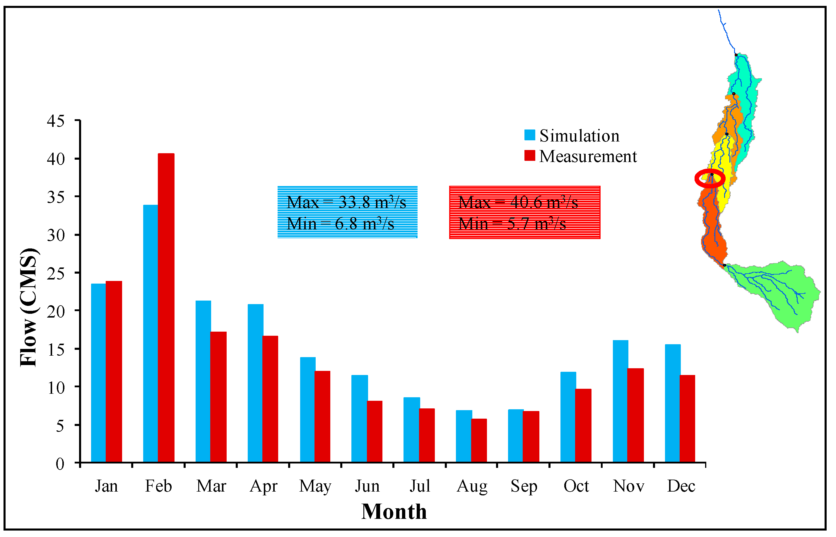
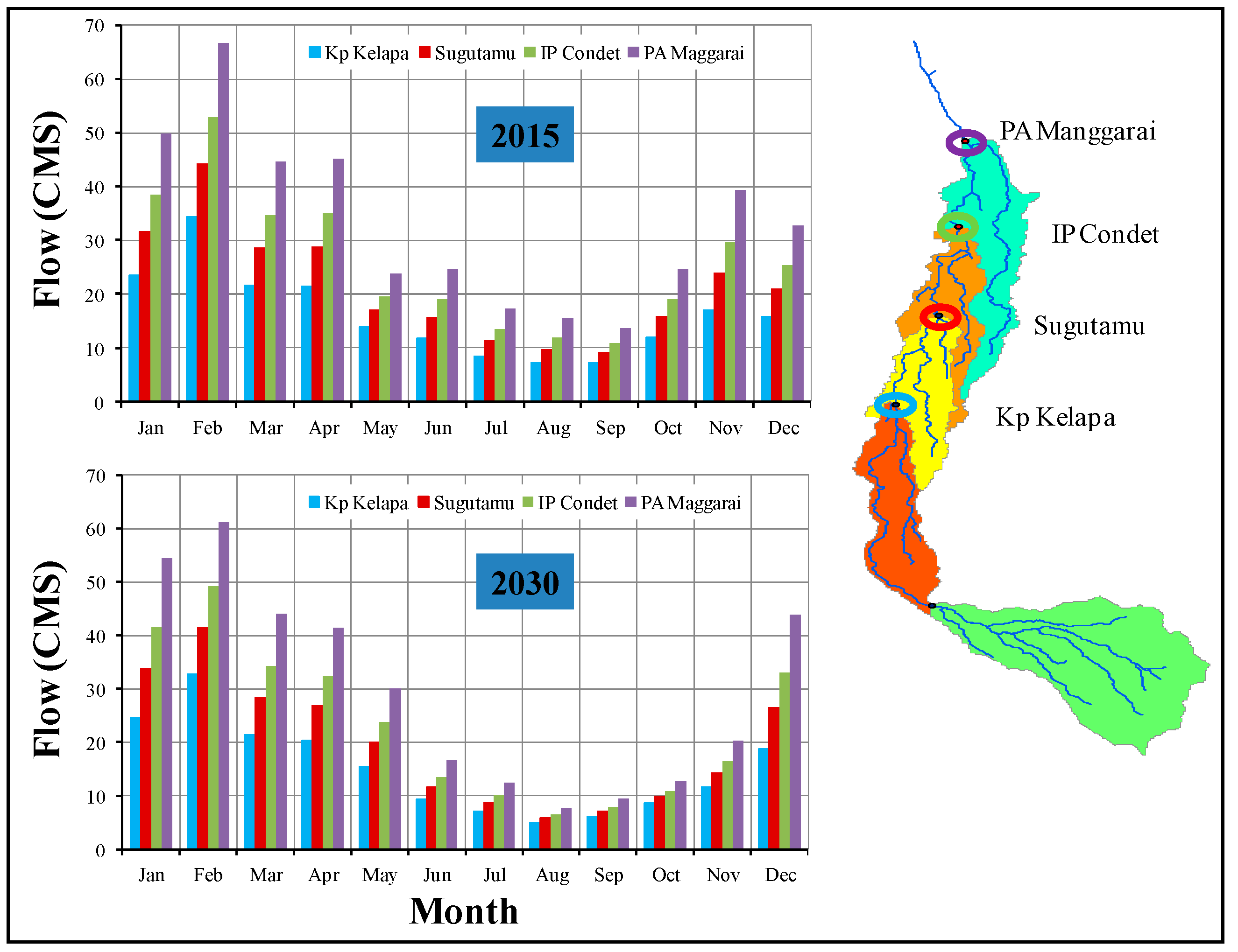
In this study, effect of climate change is mainly shown through change in rainfall pattern. A graph showing the comparative monthly rainfall pattern for both 2015 and 2030 with statistical significance (correlation coefficient (R2) = 0.86, root-mean-square error (RSME) = 0.28) is presented in Figure 5. With the maximum and minimum values of average monthly rainfall patterns in 2030, it clearly shows a changing pattern with lesser precipitation during dry days and higher precipitation during the shorter time period (Figure 5). With this it can be stated that frequency of extreme weather conditions such as drought as well as flooding is likely to be increased. Before conducting a future scenario analysis, the performance of the WEAP simulation is verified, with significant correlation between the observed and simulated values of water quality parameters. The hydrology module simulation performance was evaluated for the period from 2001 to 2014. Adjustments to hydrology module parameters were made with consideration of both quantitative and qualitative evaluation of the hydrologic response at the Katulampa command area or monitoring station. Different hydrological parameters (mainly effective precipitation and runoff/infiltration) were adjusted to calibrate the model and reproduce the observed monthly stream flows (Table 3). Figure 6 compares the average monthly simulated and observed stream flows between 2000 and 2007 at Kp Kelapa and shows that they largely match for most months, with an average error of 11%. Using simulated and validated future climatic variables, river discharge was simulated with the WEAP model. The result for point river discharge at four different points for both 2015 and 2030 with statistical significance (R2 = 0.89, RSME = 0.26) is shown in Figure 7.

Figure 5.
A graph showing the comparison between the observed rainfall and output from general circulation model (GCM) rainfall patterns in 2015 and 2030.
Table 3.
Summary of parameters and steps used for calibration.

Figure 6.
Comparison of the simulated and observed average monthly discharges at Kp Kelapa for the period 2000–2007. (Here CMS- Cubic Meter per Second).

Figure 7.
Comparison of the observed and simulated (output from WEAP) average monthly discharge at different stations for the years 2015 and 2030.
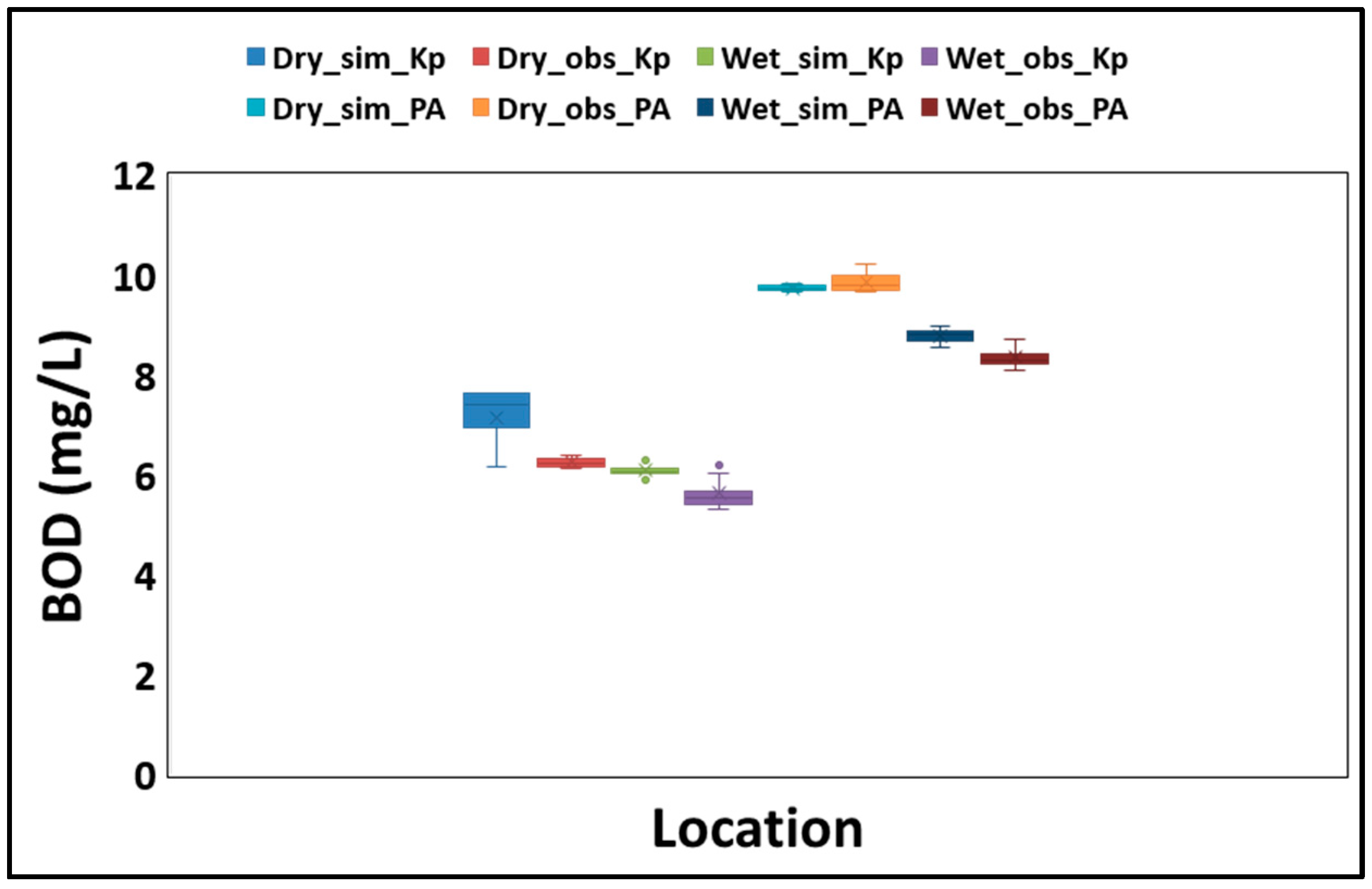
Additionally, the simulation performance of the water quality module was evaluated by comparing the BOD value for both the dry and wet seasons at two different locations, namely, Kp Kelapa and PA Mangarrai, as shown by box plot (Figure 8). The selection of these two stations and BOD as indicator was made on the basis of the consistent availability of observed water quality data for the year 2004.
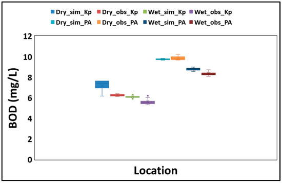
Figure 8.
Comparison of the simulated and observed BOD values during dry and wet seasons for two different locations, namely, Kp Kelapa and PA Mangarrai (year 2004). (Dry: dry season; Wet: wet season; Obs: observed value; Sim: simulated value, Kp: Kp Kelapa; PA: PA Mangarrai).
The results show a significant correlation for these observed and simulated values, and confirm the suitability of the model performance in the study area. The ranges of observed data for the dry and wet periods were 6.14–6.39 mg/L, and 5.33–6.20 mg/L for Kp Kelapa, and 9.62–10.23 mg/L and 8.10–8.72 mg/L for PA Mangarrai, respectively. On the other hand, ranges for simulated values for dry and wet periods were 6.17–7.76, and 5.91–6.30 mg/L for Kp Kelapa, and 9.67–9.81 and 8.55–8.97 mg/L for PA Mangarrai, respectively.
4.2. Future Simulation and Scenario Analyses
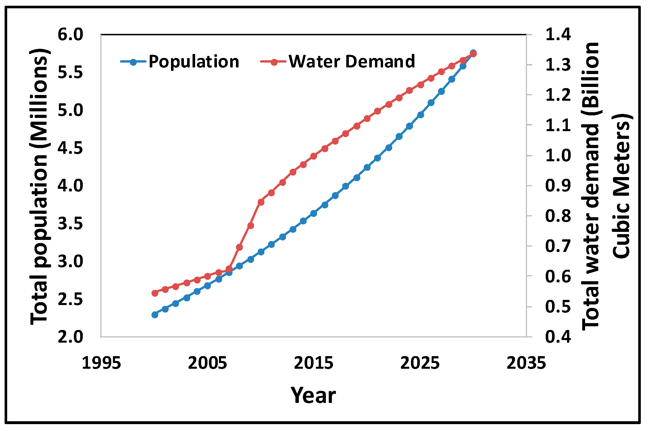
A simulation was conducted for water demand based on projected population growth for the year 2030 to get an overall impression about water scarcity. The result for total water demand is shown in Figure 9 and indicates that the annual water demand for the year 2030 will be approximately 1.34 billion m3, which is approximately 2.5 times that for 2000, i.e., 0.55 billion m3. This rapid rate of increase in demand should encourage water planners to take appropriate action in due course of time for sustainable management for future generations.
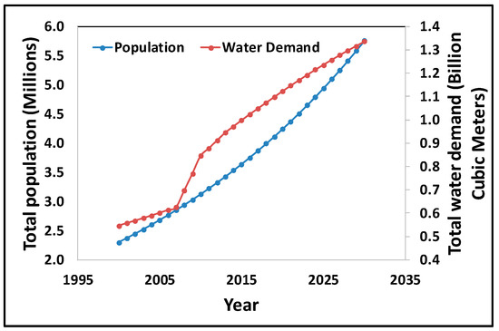
Figure 9.
The simulation result for total water demand in the study area.
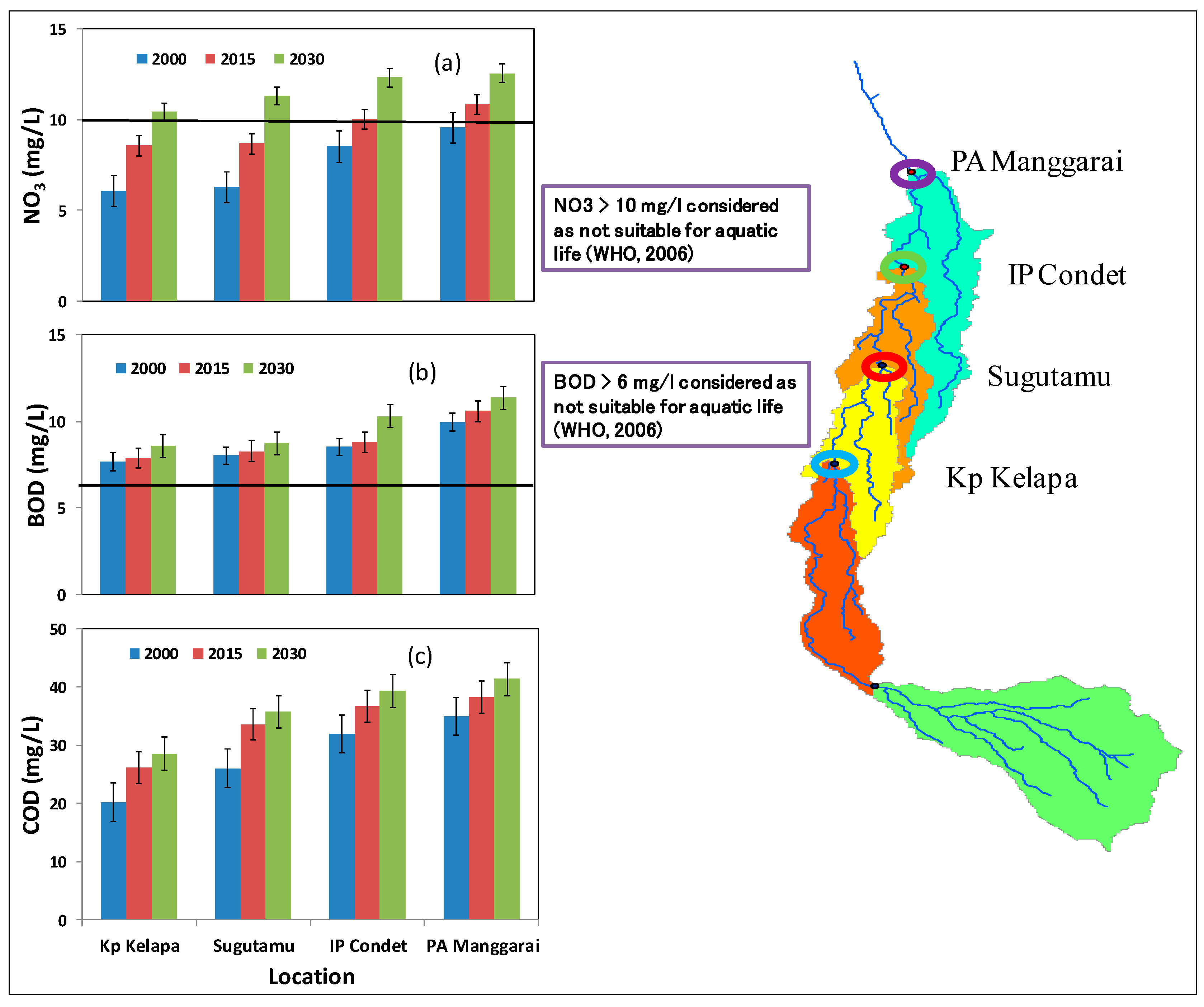
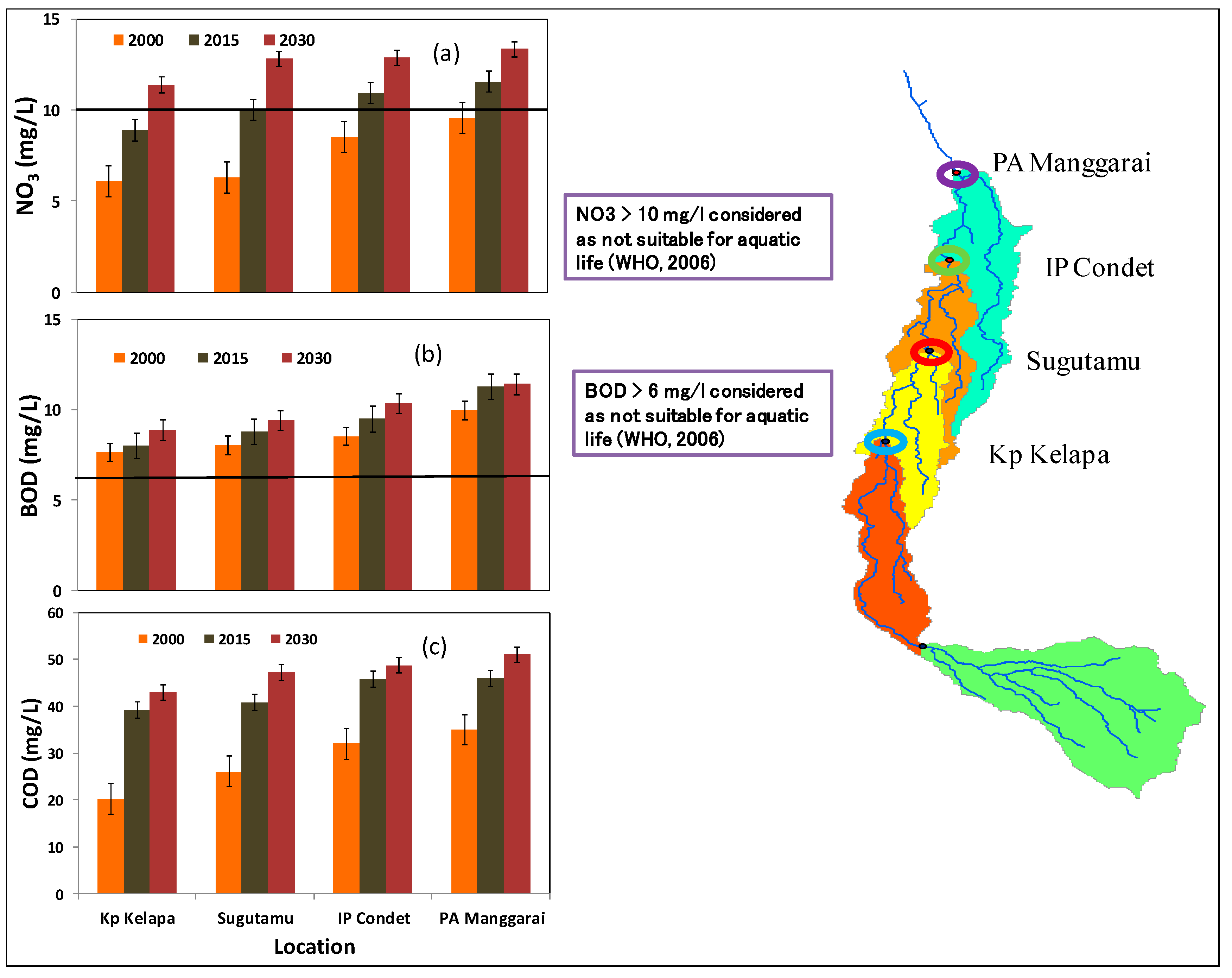
In the next phase, future simulation of water quality using selected parameters (NO3, BOD and COD) was conducted under two different scenarios, first, with population growth and planned expansion of current wastewater management infrastructure by 2030, and second, considering the effect of climate change along with population growth and wastewater management infrastructure. The idea behind running these two scenarios is to obtain a deep insight for possible policy intervention and provide a potential solution for water-related problems. Spatio-temporal simulation and prediction of water quality parameters was conducted for 2015 and 2030 using 2000 as a reference or base year. The simulation results for the water quality parameters using these two scenarios are shown in Figure 10 and Figure 11, respectively. Here, vertical black lines represent standard deviation in the data set which is statistically significant. Based on the water quality parameters, the general trend showed that water quality deteriorates from upstream to downstream because of the addition of an anthropogenic output (sewerage). Additionally, the magnitude of deterioration is of higher order in the case of the second scenario where climate change has an additional effect. The reason for this may be the high frequency of extreme weather events due to climate change in the second scenario. Here extended dry period because of climate change (low flow period in the rivers), might be one of drivers for increasing the concentration of contaminants. Explaining water quality more precisely, a high concentration of nitrate indicates the influence of agricultural activities, fertilizer use, microbial mineralization, untreated sewerage input, and animal waste. In general, most of the water samples are safe for the aquatic system in terms of NO3, except for at the PA Mangarrai location. However, with regard to the development with the climate change scenario, water quality will deteriorate at the other locations as well. The value for BOD varies from 7.65 to 11.35 mg/L, which clearly indicates that all the water samples are moderately to extremely polluted with reference to the BOD required value for a safe aquatic system, i.e., 6 mg/L [35]. The COD value, a commonly used indicator of both organic and inorganic nutrients in water samples, increases when extended into the future. The above result suggests that current management policies and near future water resources management plan are not enough to maintain the pollution level within the desirable limit and calls for transdisciplinary research in more holistic way for doing it sustainably.

Figure 10.
The simulation results of the annual average values of (a) NO3, (b) BOD and (c) chemical oxygen demand (COD) for four different locations in 2000, 2015 and 2030 (scenario considering population growth and planned wastewater infrastructure for 2030). (Here, WHO- World Health Organization).
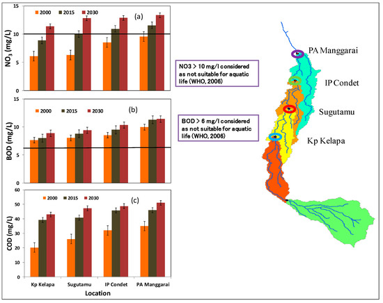
Figure 11.
The simulation results of the annual average values of (a) NO3, (b) BOD and (c) COD for four different locations in 2000, 2015, and 2030 (scenario considering population growth and climate change with planned wastewater infrastructure for 2030).
5. Conclusions
This research examined the status of current and future water resource quality and quantity under different scenarios. The significant correlation between the simulated and observed values indicate that the hydrology and water quality modules in the WEAP model can efficiently replicate stream flows and water quality variables. Based on an exponential increase in the total demand of water resources, promotion of water reuse and water recycling in industries can also contribute toward restoration and reclamation of water resources and can reduce urban water demand. The results of the simulated water quality clearly indicate that it is moderately to extensively polluted throughout the Ciliwung River basin. The average rates of deterioration because of population growth for NO3, BOD and COD are 53.03%, 14.10%, and 28.15%, respectively, from the base year 2000. However, with addition of climate change, the rates of deterioration were 65.62%, 17.14% and 67.97%, respectively. Additionally, the simulation result indicates that the rate of further deterioration in the near future is quite high because the current WWTP plans for the year 2030 are largely inadequate for tackling an increase in the wastewater production from population outburst and the extreme weather conditions due to climate change. Results from this work will be useful for local stakeholders involved in the water sector in order to formulate strategic and adaptive plans for the future. This suggests that consideration of both climate change and non-climate-related changes must be inclusively incorporated in policy planning for better adaptation and sustainable water resource management. This may include better regulation for wastewater treatment (with both short- and long-term population growth in mind), sectoral water usage practices based on water quality, proper management of non-revenue water loss, conjunctive use of surface and groundwater and consideration of extreme weather conditions.
Supplementary Materials
Supplementary File 1Acknowledgments
The authors would like to acknowledge the support of the Water and Urban Initiative (WUI) project of the United Nations University Institute for the Advanced Study of Sustainability (UNU-IAS) for financial and other logistic assistance in conducting this research.
Author Contributions
Pankaj Kumar developed the methodology, did all the research analysis and wrote the manuscript. Yoshifumi Masago and Binaya Kumar Mishra helped in refining the methodology and result part. Shokhrukh Jalilov, Ammar Rafiei Emam, Mohamed Kefi and Kensuke Fukushi helped in writing and formatting whole manuscript.
Conflicts of Interest
All authors acknowledge that there is no conflict of interest here.
References
- United Nations Environment Programme (UNEP). The UN-Water Status Report on the Application of Integrated Approaches to Water Resources Management. Available online: http://www.unwater.org/publications/un-water-status-report-application-integrated-approaches-water-resources-management-rio20/ (accessed on 12 August 2012).
- Bos, R.; Alves, D.; Latorre, C.; Macleod, N.; Payen, G.; Roaf, V.; Rouse, M. Manual on the Human Right to Safe Drinking Water and Sanitation for Practitioners; IWA Publications: London, UK, 2016; p. 120. [Google Scholar]
- Asefa, T.; Clayton, J.; Adams, A.; Anderson, D. Performance evaluation of a water resources system under varying climatic conditions: Reliability, resilience, vulnerability and beyond. J. Hydrol. 2014, 508, 53–65. [Google Scholar] [CrossRef]
- Goharian, E.; Burian, S.; Bardsley, T.; Strong, C. Incorporating Potential Severity into Vulnerability Assessment of Water Supply Systems under Climate Change Conditions. J. Water Resour. Plan. Manag. 2015. [Google Scholar] [CrossRef]
- Zimmerman, J.B.; Mihelcic, J.R.; Smith, J. Global stressors on water quality and quantity. Environ. Sci. Technol. 2008, 42, 4247–4254. [Google Scholar] [CrossRef] [PubMed]
- Malsy, M.; Flörke, M.; Borchardt, D. What drives the water quality changes in the Selenga Basin: Climate change or socio-economic development? Reg. Environ. Chang. 2016, 1–13. [Google Scholar] [CrossRef]
- United Nations World Water Assessment Programme (WWAP). The United Nations World Water Development Report 2015: Water for a Sustainable World; UNESCO: Paris, France, 2015. [Google Scholar]
- Goharian, E.; Burian, S.J.; Lillywhite, J.; Hile, R. Vulnerability assessment to support integrated water resources management of metropolitan water supply systems. J. Water Resour. Plan. Manag. 2017, 143, 3. [Google Scholar] [CrossRef]
- Karamouz, M.; Goharian, E.; Nazif, S. Reliability Assessment of the Water Supply Systems under Uncertain Future Extreme Climate Conditions. Earth Interact. 2013, 17, 1–27. [Google Scholar] [CrossRef]
- Hughes, D.A.; Kapangaziwiri, E.; Mallroy, S.J.L.; Wagener, T.; Smithers, J. Incorporating Uncertainty in Water Resource Simulation and Assessment Tools in South Africa; WRC Report No. 1838/1/11; Water Research Commission: Pretoria, South Africa, 2011. [Google Scholar]
- Pappenberger, F.; Beven, K.J. Ignorance is bliss: Or seven reasons not to use uncertainty analysis. Water Resour. Res. 2006, 42, W05302. [Google Scholar] [CrossRef]
- Beven, K.J.; Alcock, R.E. Modelling everything everywhere: A new approach to decision-making for water management under uncertainty. Freshw. Biol. 2012, 57, 124–132. [Google Scholar] [CrossRef]
- Jin, H.; Zhu, Q.; Zhao, X.; Zhang, Y. Simulation and prediction of climate variability and assessment of the response of water resources in a typical watershed in China. Water 2016, 8, 490. [Google Scholar] [CrossRef]
- McIntyre, N.R.; Wheater, H.S. A tool for risk-based management of surface water quality. Environ. Model. Softw. 2004, 19, 1131–1140. [Google Scholar] [CrossRef]
- Kumar, P.; Kumar, A.; Singh, C.K.; Saraswat, C.; Avtar, R.; Ramanathan, A.L.; Herath, S. Hydrogeochemical Evolution and Appraisal of Groundwater Quality in Panna District, Central India. Expo. Health 2016, 8, 19–30. [Google Scholar] [CrossRef]
- Deksissa, T.; Meirlaen, J.; Ashton, P.J.; Vanrolleghem, P.A. Simplifying dynamic river water quality modelling: A case study of inorganic dynamics in the Crocodile River, South Africa. Water Air Soil Pollut. 2004, 155, 303–320. [Google Scholar] [CrossRef]
- Cox, B.A. A review of currently available in-stream water-quality models and their applicability for simulating dissolved oxygen in lowland rivers. Sci. Total Environ. 2003, 314–316, 335–377. [Google Scholar] [CrossRef]
- Radwan, M.; Willems, P.; El-Sadek, A.; Berlamont, J. Modelling of dissolved oxygen and biochemical oxygen demand in river water using a detailed and a simplified model. Int. J. River Basin Manag. 2003, 1, 97–103. [Google Scholar] [CrossRef]
- Sieber, J.; Purkey, D. Water Evaluation and Planning System. User Guide for WEAP21; Stockholm Environment Institute, U.S. Center: Somerville, MA, USA, 2011; Available online: http://www.weap21.org/ (accessed on 1 April 2014).
- Ingol-Blanco, E.; McKinney, D. Development of a Hydrological Model for the Rio Conchos Basin. J. Hydrol. Eng. 2013, 18, 340–351. [Google Scholar] [CrossRef]
- Slaughter, A.R.; Mantel, S.K.; Hughes, D.A. Investigating possible climate change and development effects on water quality within an arid catchment in South Africa: A comparison of two models. In Proceedings of the 7th International Congress on Environmental Modelling and Software, San Diego, CA, USA, 15–19 June 2014; Ames, D.P., Quinn, N.W.T., Rizzoli, A.E., Eds.; ISBN 978-88-9035-744-2. [Google Scholar]
- Assaf, H.; Saadeh, M. Assessing water quality management options in the Upper Litani Basin, Lebanon, using an integrated GIS-based decision support system. Environ. Model. Softw. 2008, 23, 1327–1337. [Google Scholar] [CrossRef]
- Cook, C.; Bakker, K. Water security: Debating an emerging paradigm. Glob. Environ. Chang. 2012, 22, 94–102. [Google Scholar] [CrossRef]
- Ravesteijn, W.; Kop, J. For Profit and Prosperity: The Contribution Made by Dutch Engineers to Public Works in Indonesia, 1800–2000; Koninklyk Instituut Voor Taal Land: Leiden, The Netherlands, 2008; p. 563. [Google Scholar]
- Amato, C.C.; McKinney, D.C.; Ingol-Blanco, E.; Teasley, R.L. WEAP Hydrology Model Applied: The Rio Conchos Basin, Center for Research in Water Resources; The University of Texas: Austin, TX, USA, 2006; Available online: https://repositories.lib.utexas.edu/handle/2152/7025 (accessed on 15 July 2014).
- Australian Aid. East Asia Pacific Region Urban Sanitation Review: Indonesia Country Study; World Bank Group: Washington, DC, USA, 2013; p. 68. [Google Scholar]
- Esteve, P.; Varela, C.O.; Blanco, I.G.; Downing, T.E. A hydro-economic model for the assessment of climate change impacts and adaptation in irrigated agriculture. Ecol. Econ. 2015, 120, 49–58. [Google Scholar] [CrossRef]
- Sunyer, M.A.; Hundecha, Y.; Lawrence, D.; Madsen, H.; Willems, P.; Martinkova, M.; Vormoor, K.; Bürger, G.; Hanel, M.; Kriauciuniene, J.; et al. Inter-comparison of statistical downscaling methods for projection of extreme precipitation in Europe. Hydrol. Earth Syst. Sci. 2015, 19, 1827–1847. [Google Scholar] [CrossRef]
- Christensen, J.H.; Boberg, F.; Christensen, O.B.; Lucas-Picher, P. On the need for bias correction of regional climate change projections of temperature and precipitation. Geophys. Res. Lett. 2008, 35, L20709. [Google Scholar] [CrossRef]
- Hansen, J.W.; Challinor, A.; Ines, A.; Wheeler, T.; Moron, V. Translating climate forecasts into agricultural terms: Advances and challenges. Clim. Res. 2006, 33, 27–41. [Google Scholar] [CrossRef]
- Mishra, B.K.; Herath, S. Assessment of Future Floods in the Bagmati River Basin of Nepal Using Bias-Corrected Daily GCM Precipitation Data. J. Hydrol. Eng. 2014. [Google Scholar] [CrossRef]
- Elshamy, M.E.; Seierstad, I.A.; Sorteberg, A. Impacts of climate change on Blue Nile flows using bias-corrected GCM scenarios. Hydrol. Earth Syst. Sci. 2009, 13, 551–565. [Google Scholar] [CrossRef]
- Intergovernmental Panel on Climate Change (IPCC). Climate Change 2014: Synthesis Report. In Contribution of Working Groups I; II and III to the Fifth Assessment Report of the Intergovernmental Panel on Climate Change; Core Writing Team, Pachauri, R.K., Meyer, L.A., Eds.; IPCC: Geneva, Switzerland, 2014; p. 151. [Google Scholar]
- Bowie, G.L.; Mills, W.B.; Porcella, D.B.; Campbell, C.L.; Pagenkopf, J.R.; Rupp, G.L.; Johnson, K.M.; Chan, P.W.H.; Gherini, S.A. Rates, Constants and Kinetics Formulations in Surface Water Quality Modeling, 2nd ed.; EPA 600/3-85/040; US EPA: Athens, GA, USA, 1985.
- World Health Organization. Global Water Supply and Sanitation Assessment 2000 Report; WHO and UN Children’s Fund: New York, NY, USA, 2000. [Google Scholar]


© 2017 by the authors. Licensee MDPI, Basel, Switzerland. This article is an open access article distributed under the terms and conditions of the Creative Commons Attribution (CC BY) license (http://creativecommons.org/licenses/by/4.0/).