
Evaluating Flood Exposure for Properties in Urban Areas Using a Multivariate Modelling Technique
by
Geir Torgersen
1,2,*, 
Jan Ketil Rød
3,
Knut Kvaal
1,
Jarle T. Bjerkholt
4 and
Oddvar G. Lindholm
1 1
Faculty of Science and Technology, Norwegian University of Life Sciences, 1430 Ås, Norway
2
Faculty of Engineering, Østfold University College, 1671 Kråkerøy, Norway
3
Department of Geography, Norwegian University of Science and Technology, 7491 Trondheim, Norway
4
University College of Southeast Norway, 3603 Kongsberg, Norway
*
Author to whom correspondence should be addressed.
Water 2017, 9(5), 318; https://doi.org/10.3390/w9050318
Submission received: 9 March 2017
/
Revised: 11 April 2017
/
Accepted: 25 April 2017
/
Published: 1 May 2017
Abstract
:Urban flooding caused by heavy rainfall is expected to increase in the future. The main purpose of this study was to investigate the variables characterizing the placement of a house, which seem to have an impact when it comes to the exposure to floods. From the same region in Norway, data from 347 addresses were derived. All addresses were either associated with insurance claims caused by flooding or were randomly selected. A multivariate statistical model, Partial Least Square Regression (PLS), was used. Among others, the analysis has shown that the upstream, sealed area is the most significant variable for characterizing properties’ exposure to urban flooding. The model confirms that flooding tends to occur near old combined sewer mains and in concave curvature, and houses located in steep slopes seem to be less exposed. Using this method, it is possible to rank and quantify significant exposure variables contributing to urban floods within a region. Results from the PLS-analysis might provide important input to professionals, when planning and prioritizing measures. It can also predict flood-prone areas and make residents aware of the risks, which may induce them to implement preventive measures.
1. Introduction
Urban flooding caused by extreme rainfall is exacerbated by insufficient drainage and sewer systems. This type of flooding has received less attention than other floods, due to the smaller scale of individual events [1], despite the fact that in the UK, 16,000 properties are at risk of sewer flooding in the course of a decade. In the UK, these floods, caused by short-duration events, could increase from 200,000 in the present year to 700,000–900,000 in 2080 [2]. In 2007, the insurance companies in Norway estimated that the costs of urban flooding in Norway could increase by 40% or more over the next ten years [3]. When adjusted for inflation, the overall cost for precipitation damages during 2012-2014 has proven to be 46% higher compared to 2008-2010 [4].
Numerous variables have an impact on the risk of flooding. Recent literature regards the total risk as a composition of Hazard, Vulnerability, and Exposure, and they can be used as a framework to group relevant variables [5,6,7]. When it comes to the frequency, intensity, and duration of rainfall, they can all characterize the weather extremes and be linked to the Hazard of floods. The level of risk also depends on the Vulnerability and Exposure, explained respectively as how to cope with the floods and the places that will potentially be affected. The total risk can decrease by focusing on the adverse impact from all kinds of variables, and in a more comprehensive model, it should be possible to add variables from any of these three groups.
Traditionally, studies regarding urban floods include dynamic, hydraulic modelling, dealing with the speed and volume of flooded water and intended to determine exposed areas. This study highlights the exposure to floods, as we use a database of addresses where flooding has occurred as a basis. In this study, we conducted a statistical analysis on GIS generated terrain variables linked to addresses. Whether a house has been flooded or not can be regarded as a response variable for a complex set of parameters. The present research was designed by using Partial Least Square regression (PLS) on two sets of addresses. The first group had experienced urban flood events during the years 2006–2012. All selected claims occurred due to rainfall and had a link to the sewer system. The second consisted of randomly selected addresses from the same region. For each sample, 38 variables were used in a multivariate model.
The purpose of this study was two-fold:
- Develop a multivariate model to identify and rank significant variables contributing to the exposure to urban flooding;
- To develop a model to quantify areas prone to urban flooding.
There are, to our knowledge, no other studies using a multivariate model, such as a PLS model, to identify and rank significant variables contributing to urban floods. Some other studies investigating insurance claims and rainfall data have been carried out, but mostly on an aggregated district-level. In a study from the Netherlands and Denmark, a weak relationship was found between property damage and recorded heavy rainfall for summer events, indicating that rain events mainly induce claims the same day [8,9]. Another study [10] concluded that local rainfall statistics were not able to describe the individual cost per claim. However, it was suitable for modelling the overall cost per day. Spekkers et al. [11] used district-aggregated claims to analyze factors influencing urban flooding. They found that claims are most strongly associated with the maximum hourly rainfall intensity followed by the real-estate value, building area, income, household income, and age of the building. Merz et al. [12] stated that to develop reliable damage models, there is a need for more multivariate statistical analyses to look for patterns and interactions between various parameters affecting urban areas.
2. Materials/Access to Data
2.1. Case Area
Fredrikstad is a city with close to 80,000 inhabitants and is situated in Southeastern Norway by the estuary of the river Glomma. The municipal area is 290 km2, with a relatively long coastline to the Oslo fjord. According to Norwegian standards, it is densely populated.
Fredrikstad’s landscape consists of small valleys and hills that are mainly oriented north-south. The river Glomma also runs north-south and through Fredrikstad, where it frequently causes fluvial flooding [13]. The soil is dominated by clay and there is exposed bedrock in several places throughout the city area, contributing to the amount of impermeable surface areas. In combination with a high groundwater level, this lowers the potential for the infiltration of storm water. Sewers are often located along the lowermost part of the valleys and will often be filled by surface water from the hillsides [14,15].
Indeed, in recent years, the region has experienced numerous pluvial flood events. In the early 2000s, several insurance companies held the municipalities responsible for the damages due to the limited capacity of the sewers and took legal action for a recourse of their pay outs [16]. Heavy rain events in 2006–2008 triggered a similar trial, which ended in a settlement between the two parties. In 2007, a general plan for storm water management in Fredrikstad was launched. One of the intentions of the plan was to create awareness among developers regarding sustainable storm water solutions [17]. Against this background, Fredrikstad was a particularly interesting case for this study.
2.2. Insurance Data
Insurance companies are among those that most rapidly experience the economic consequences of urban flooding, and they initially have to pay compensation for most damages due to floods. For water-related damages in Norway the recent years, only a minor part of the payments were natural hazards, as defined and covered by the Norwegian Natural Perils Pool [18].
The appraisers from most of the insurance companies in Norway are required to use predefined codes to classify the claim as a part of the documentation process. This national database was standardized in 2006 and is administered by Finance Norway, which is the industry organisation for the financial industry in Norway. The market share for the insurance companies using the system in Norway is approximately 90%. All water-related data are coded in three categories [19]:
- Installation: A description of where the malfunction that has led to the damage is located, e.g., water pipes indoor, outdoor, sewer mains;
- Source: A description of the underlying reason for the damage, e.g., precipitation, water supply;
- Cause: Describes the actual cause for the damage, e.g., stop in sewers, aging, frost, malfunction.
Municipalities do not have regular access to Finance Norway’s database of registered flood events on a detailed level. Hence, they have to create their own records to achieve an overview. Information is obtained from their own investigations, mainly based on random contact with residents or from recourse cases. This information has thus become very important when prioritizing flood preventive measures. As a part of Finance Norway's dedication to prevent climate-related damages (or any damage that leads to a claim), their database has been made available for selected research purposes, like this study. Claims specified on addresses are sensitive information, both with respect to personal information and for competitive reasons among insurance companies. Thus, permission was required to obtain access to this data. For this study, the following key-parameters have proven useful:
- Address (property where the damage occurred);
- Compensation sum;
- Classification into codes for Installation, Source, and Cause.
2.3. Geocoding
Geocoding is the process of assigning coordinates to units in a table based on spatial information such as street addresses. Building central points (BCP) is an extract from the Norwegian cadaster, and each point represents a building with a unique address. We used the BCPs to geocode all addresses in the sample. By matching the addresses with the official register (the national cadaster), the coordinates were found. Furthermore, by using text-matching algorithms in pythontm (programming language), these units were geocoded. Once the records in a table are geocoded, they add value to the analysis as it is a very effective method for the generation of environmental variables describing the local morphology surrounding the buildings.
2.4. Terrain Parameters
A geographic information system (GIS) was used to generate terrain representations and from these, the terrain variables were extracted. Terrain is commonly represented in GIS using the raster format, where the entire study area is tessellated into a quadratic cell. We generated terrain parameters from digital elevation models (DEM) at three different resolutions (cell sizes): 1, 10, and 50 m, and generated slope and curvature rasters from these. Figure 1 shows the slope values for a small part of Fredrikstad and the inset map is zoomed in on one of the points, representing one of the buildings from the sample. The building point is located within a cell with a slope value of 13.05 degrees, which is the value being assigned as the unit for this variable. However, the location of the building may be anywhere within the cell and possibly towards its edge (as in the inset map in Figure 1). Another variable was added where the slope value was a distance weighted mean of the four nearest pixel values (which in this case equals 18.46). Variables taking the nearest cells into account are referred to as interpolated values.
For this study, we have used “Terrain parameters” as a generic term for variables characterizing the location in the field. The selected parameters were all assumed to be flood relevant and divided into four groups:
- Distance (elevation z, distance to coast). This group includes the altitude above mean sea level (z) and distance to the coast measured from each building’s central points (BCP);
- Slope (the slope gradient) includes the slope value from the cells. The variable sl_r100 gives the mean slope within a 100-meter radius for an area elevated higher than the BCP. The other slope values are derived from the cells at the three different resolutions mentioned above;
- Area (permeable, impermeable, and sum) was derived from the BCP and arranged in the contributing area into permeable and impermeable surface areas, all within a 100 m radius from the BCP. The upstream sealed area shown in Table 1 was calculated in two ways (abbreviations are explained in Table 1): One includes roads elevated higher than the BCP (a_Up_ro) and another includes all upstream built-up areas (a_US_im) according to [20]. When calculating an upstream area, all cells elevated higher than the BCP were included. This is a limitation, as not all those cells will drain through the BCP. A more accurate way to calculate the upstream drain area might be an opportunity for improvement in further studies. These variables were calculated in a similar way, and we considered that this simplification would not led to statistical bias;
- Curvature profile (plan and profile). Terrain curvature is expressed as the plan or profile curvature, measured along the steepest descent and the contour, respectively. The curvature number is also known as the second derivate value of the input surface by cells, based on the algorithm described by Zevenbergen and Thorne [21].
2.5. Sewer Data
In Fredrikstad, most mains are registered by several variables such as Diameter, Year of Construction, and the Sewer system. Addresses connected to the sewer mains, were either categorized as a part of a combined (single pipe) or separate (two-pipe) sewer system. The combined system dominated until the mid-1960s, when it was substituted by the separate system as an improved method. A comprehensive manual search was carried out for each address to determine the most likely point of connection to the sewer mains, including measuring the distances.
2.6. Sampling
To achieve relevant samples for this study, some inclusion criteria were necessary.
According to the code system, all claims coded Cause = Stop in Sewers/Backflow were selected. These claims are particularly interesting for the municipalities due to the link to sewer mains [22]. There is a possibility that some of these claims are due to other reasons than the mains, e.g., damages or blockage of service pipes. In order to eliminate this, only claims coded as Source = Precipitation were selected. Similarly, a random sample was generated as a reference sample, representing “normal” addresses throughout the case area.
The BCP from the cadaster for the Fredrikstad municipality represented a pool of points from where a random sample was created using the tool Create Random Points available in the ArcGIS® 10.3 software (ESRI, Redlands, CA, USA).
Damage data from the insurance companies were supposed to have locational information such as the street address and unique building identifiers. Of the claims within the inclusion criteria, about 65% unique building identifiers were found and coded. Abbreviations and misspellings were common, but caused no problems.
For this study, it was important to assess the connection point where buildings with a reasonable certainty were linked to the sewer mains. This information is not yet represented as a GIS-layer and variables were therefore generated manually. For 12% of all selected addresses (mainly in the rural area), it turned out to be impossible to determine the connection point to the mains. Finally, some addresses reported as flooded and caused by the sewer, proved to be elevated high above the sewer system. It was unlikely that the sewer mains should have had an impact of these floods. Based on available map information, it was only possible to estimate the vertical distance in integer meters. A threshold was set, and thus all addresses >2 m from the BCP-level to the ground above the sewer mains were eliminated from the dataset. This proved to be 5% of all flooded addresses.
Finally, the dataset consisted of 179 flooded and 168 random addresses. With one exception, random addresses were non-flooded. One single address appeared to be included in both groups and is therefore given special attention in the results section.
3. Method
A goal of this work was to use a set of independent variables linked to each address to predict whether an object belonged to one of two classes (flooded or randomized properties). For this purpose, Partial Least Square Regression (PLS) was chosen. As there were two classes of interest in this study, a special case called Partial Least Square-Discriminant Analysis (PLS-DA) was preferred.
PLS was also found to be suitable due to the high collinearity in the dataset, which may lead to poor results if using, e.g., Ordinary Least Square regression (OLS) [23,24]. Other methods such as Principal Component Analysis (PCA) reduce the number of dimensions and describe the overall variation in the dataset, but only capture the characteristics of the predictors (X). In PLS, the emphasis is on the prediction of the responses (Y). PLS was originally developed as a technique in econometrics, but today, it is primarily used as a tool for chemometrics. Occasionally, PLS is used for environmental studies in order to investigate patterns among variables in environmental studies [25,26]. The software Unscrambler® version 10.3 (CAMO Software AS, Oslo, Norway) was used for this analysis [27].
The dataset for this study consisted of 347 variables. The addresses (X-matrix) had 38 observed feature variables, while the Y-matrix had two classes (flooded or random).
Initially, the PLS-regression started by scaling and constructing linear combinations of the predictors (X) and responses (Y). From the PLS-algorithm, both X and Y matrices were decomposed into matrices of scores and loadings. In PLS, the decomposition process was finalized when the linear combination of the predictors reached its maximum covariance with the responses. In general algebraic terms, this can be written as:
P and Q are the loadings and E and F are the residuals (errors) of the X and Y matrices, respectively. The original dataset of X was regressed into t-scores T, which in turn, were used to predict the u-scores U. Finally, the u-scores were used to predict the responses Ŷ.
To assess the properties for the PLS model, validation was required. As the number of samples was considered to be small, a full cross validation of the dataset was found to be a proper method, as long as the predicted object was not used in the development of the model [28]. During the cross-validation, the dataset was divided into 20 segments. Each segment was left out from the calibration dataset and the model was then calibrated for the remaining objects. Then, the values for the left-out objects were predicted and the residuals were calculated. This process was repeated with another subset of the calibration set until all the segments had been left out once [27].
An approach to solving classification problems is the use of linear regression with dummy responses [29]. This is a binary linear classification (flooded and random). The dummy matrix Y (n × 2) can be defined as:
Furthermore, the scores from the PLS model were used to assign class membership for each address. As we had two classes, the original dummy values could either be 1–0 (flooded) or 0–1 (random). The model predicted two ŷ-values and Σŷi=1. An often used approach for assigning the membership of a class is the “winner-takes-all-strategy” and the majority vote [30]. This means that the highest score calculated from the model obtains the class-assignment. Transferred to this study, ŷi, Flooded > ŷi, Random should be interpreted as flooded (F) and vice versa.
The software plots of each sample on a 2D map (score plot) are based on the calculated value related to the factors (latent variables) from the PLS-regression. In the plot, factor 1 will capture most of the variance, factor 2 will capture the second most, etc. In the score plot, two neighbouring samples are more similar with respect to the two factors concerned and vice versa. Likewise, objects located far from each other have different structures. In the loading plot, the predictor’s influence on the model is viewed. Adjacent variables are considered to have a high positive correlation and those in diagonally opposite quadrants tend to be negatively correlated. Plots to the far right and left along the factor-1-axis are important for the model, in contrast to those located close to the origin.
Simultaneous interpretations of scores and loadings are probably the most useful feature of a PLS-plot. A sample located to the right in the score plot usually has a large value for variables to the right in the loading plot, and vice versa. In this study, samples were labelled in the score plot, as flooded or randomized addresses. By comparing the scores and loading plot, the characteristics of the two classes can be explained [27].
4. Results
All variables used in the PLS-analysis are shown in Table 1.
In Table 1, the two classes, flooded (F) and random (R), are shown. Due to limited space for text in the plot, abbreviations were needed for labelling the samples and variables. A full label and a brief description of each variable, as well as average and Standard Deviation-values (SD), are shown in Table 1. Some distinctions appear among the classes. For example, it makes sense that flooded houses on average are lower elevated (d_z1) and more associated with a combined sewer system (se_C) than random houses (abbreviations are explained in Table 1). For this study, a PLS model was used to reveal the internal structure and the significance of the individual variables according to their sensitivity to flood-risk. To handle the input variables on a common scale during the PLS-regression, each variable was divided by its standard deviation.
In terms of classification using the winner-takes-all-strategy, 84% of initially flooded houses were correctly classified. Correspondingly, the number for randomized houses was 68%. This indicates that 32% of the random addresses tend to have the attributes of flood-prone homes. Conducting a 2 × 2 confusion matrix for the validated responses, the over all accuracy was calculated as being 76.4%. As most of the objects were correctly classified, this model was considered as reliable for further analysis.
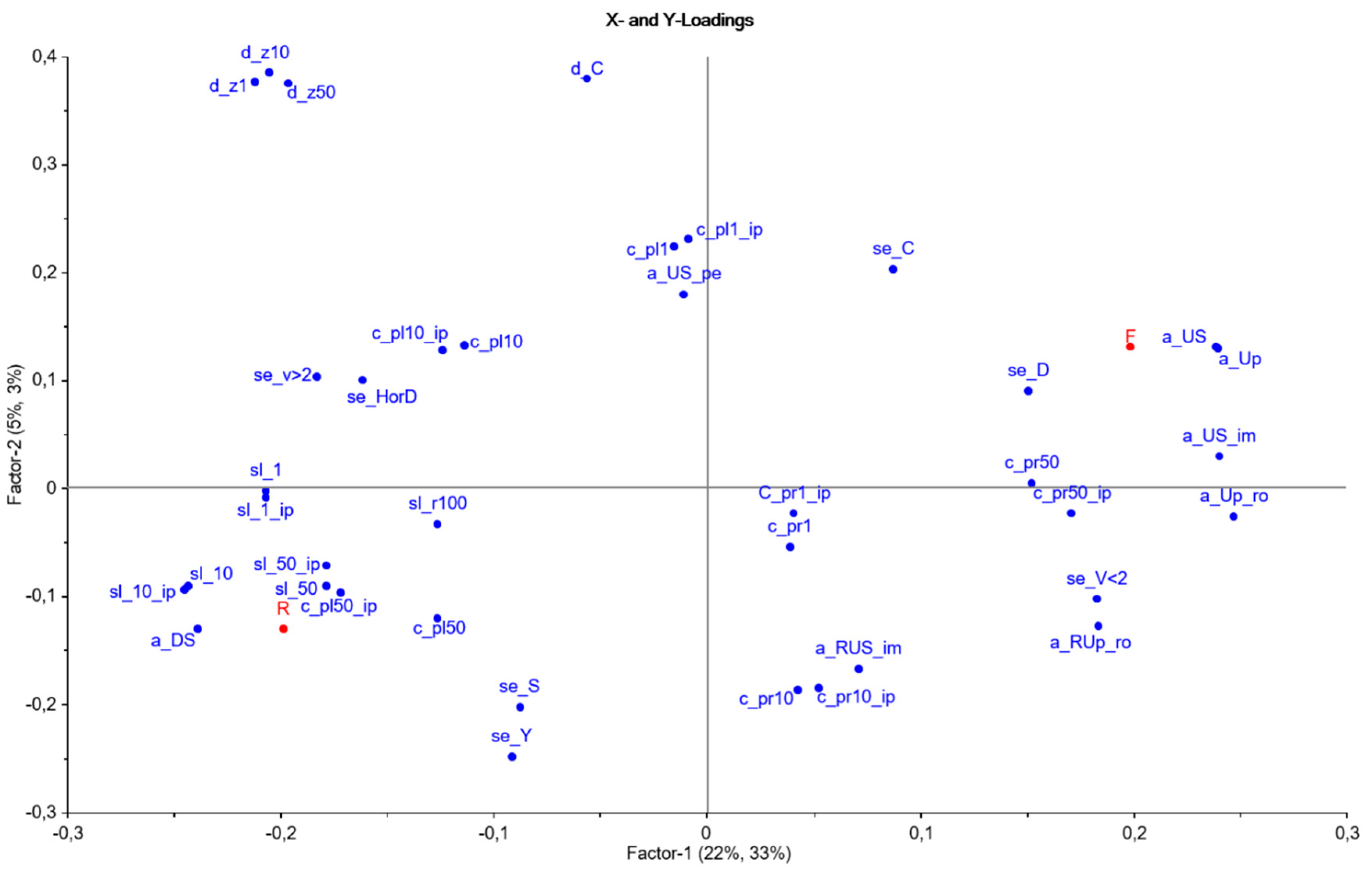
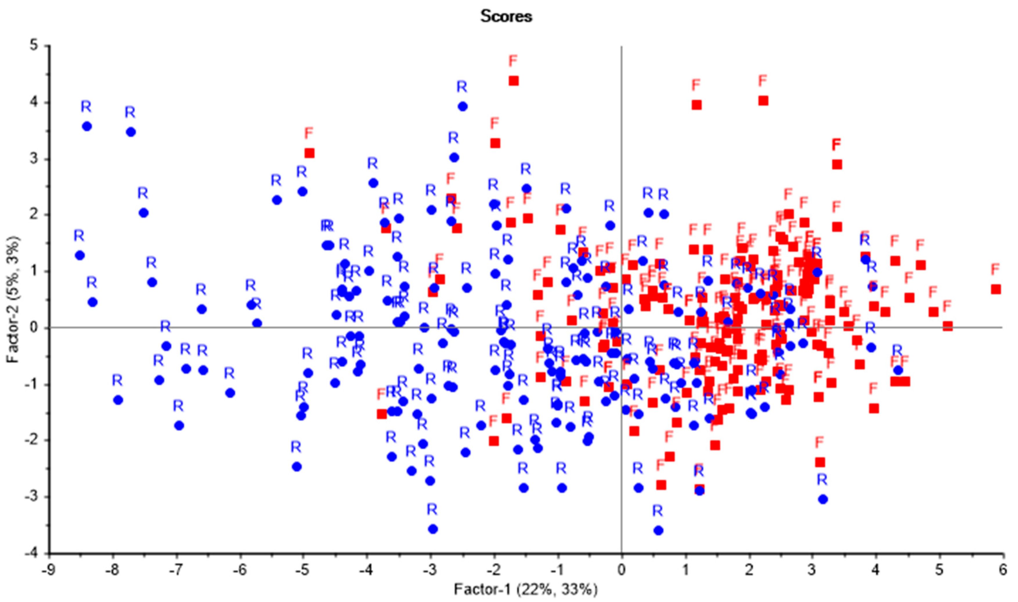
The output from the PLS-DA model in terms of the score and loading plot is shown in Figure 2. These plots form the basis of the interpretation of single variables in the discussion section. Numbers in brackets display the variance for X-data and Y-data for Factor-1 and Factor-2 (latent variables). From Figure 2, it was calculated that the first two factors in the sum described 27% and 36% of the variance in the dataset for X and Y, respectively. The explained variance for the model showed that even more factors did not capture more of the variance.
Figure 2 shows a 2D plot for Factors 1 and 2 from the PLS-regression. In the score-plot, the red-marked dots (F) are mostly located at the right-hand side (positive value of Factor 1), while most of the random data is at the left-hand side. The separation between the red and blue marked dots indicates the different structures between the two classes. This suggests that this difference is mainly explained by Factor-1. It is hard to discriminate the classes along the Factor-2 axis (or any other factors at higher levels).
As mentioned above, one single address was included in both samples. This address was plotted twice at 1.22, −2.88 in the score plot in Figure 2. As this address is exposed to flooding, it was further confirmed in the validation-process.
The loading plot in Figure 2 shows the importance of each variable in relation to Factor 1 and Factor 2. The variables derived from the upstream area are found to at the far right, while the slope, elevation, and downstream areas are found at the opposite side.
The scattered nature of the variables shown in Figure 2.
5. Discussion
An analysis of the scores and loadings in Figure 2 suggests that the rate of the impervious and upstream area surrounding the BCP is the most significant characteristic for a flood-prone property. All four variables rightmost in the loading plot belong to this group, just as flooded samples are to the right in the score plot. a_US and a_DS are inversely correlated, and this follows from the exact number of cells surrounding the BCP (abbreviations are explained in Table 1). For a given range, the area surrounding the house is equal, and thus, a large proportion of the area at a higher altitude correspondingly means a smaller area downstream. It seems that the area of permeable surfaces (a_US_pe) has little impact, as this variable is plotted close to the origin in the score plot. The plot clearly confirms a well-known phenomenon that a higher proportion of sealed areas increases the runoff and the risk of flooding. A large amount of this area is probably on built-up private grounds. Taking this into account, the municipality, both as the developer and authority, plays an important role in informing citizens and making them aware of the great impact that impermeable surfaces have on the downstream flood risk. Variables characterizing the average slope suggested that homes at risk of flooding are more often in flat areas. At steep slopes, floodwater will probably just pass the houses and do not cause any harm. Another flood-type, a flash flood, occurs when heavy rain is collected in the slopes and immediately drains to rivers that originally hold very little or no water. This can be particularly dangerous, since the water level rises suddenly and is difficult to forecast. In 2003, a so-called Flash Flood Potential Index (FFPI) was presented [31] Originally, this index was based on an equal weighting of the parameters; slope, land use, soil type, and vegetation cover. Later, the model was developed and the slope was given a slightly higher weight [32].
Variables describing distance to the sea (d_C did not seem to matter to the model. Generating this variable was intended to assess whether high tide and seawater in the sewer decrease the flow velocity and lead to flooding for houses close to the coastline. Elevation (z) turned out to be of great importance for the model and was inversely correlated with flood-prone homes. There might be two explanations for this. First, low-lying houses are simply more exposed to flooding than houses higher up. Secondly, the oldest part of the city is low-lying, with a higher portion of sealed surfaces and older sewers. The latter appears in Figure 2, as the variables measuring a dense area (a_Up_ro and a_US_im) and a combined sewer system (se_C) are located on the right side and are inversely correlated to the elevation z.
Terrain curvature determines whether a given part of a surface is convex or concave. For plan and profile curvature, the sign rules are inversely defined, and a negative and positive number, respectively, describes the concavity. Profile curvature indicates the form of the surface in the steepest direction and whether the terrain flattens into a concave curvature. The flow of surface water will lose speed and water will accumulate. Figure 2 indicates that this variable is important for a map-resolution of 50 m × 50 m and the fact that the most flood-prone areas are located in concave landscapes. The curvature number calculated for 1 DEM in Figure 2 is found close to the origin, and hence, is less significant. This indicates that when assessing the flood-risk vs. the shape of the terrain, we have to look at a slightly larger area.
The loading plot shows that the oldest sewer system (combined) with larger pipes correlates best with the flooded addresses. The random addresses are more likely to be located close to the separate sewer system. These observations are not surprising, due to the historical background of the type of sewer systems. Anyway, it should be noted that the rate of the upstream sealed area seems to have more impact on the model than the type of sewer system.
This study covers urban floods, which mainly do harm in densely populated areas, due to the lack of drainage capacity. A comparison between the FFPI-index and this study illustrates distinct differences between the two flood types. As steeper slope is characteristic of areas where a flash flood occurs, this study clearly shows that the portion of sealed surface and a little slope have more impact on pluvial floods in urban areas.
6. Conclusions
This paper highlights features of flood-prone properties in urban areas mostly caused by the insufficient capacity of the sewer system. From the PLS regression, the model predicts whether a property is prone to flood or not, with an acceptable uncertainty. The validated model correctly categorised 84% of all claims.
The variables are of different importance for the model. Even though all floods in this study are associated with the sewer system, the area in general and especially the portion of sealed surface on properties above the house, were important for the model. It makes sense that the results from the model indicate that flooding tends to occur in flat areas with a concave curvature. Furthermore, houses located on steep slopes seem to be less exposed. Possibly the most interesting aspect in this study is that the method makes it possible to rank and quantify significant variables for urban flooding. Furthermore, from the model, it is possible to predict if a property has the features of a flood-affected house. All variables in the study are related to exposure and cover only a part of all possible factors determining the flood risk. However, they are computationally fast to obtain and the result can make it easier to prioritize preventive measures, which can further contribute to a reduced flood risk.
Traditionally, the improvement of the drainage system in flooded areas means renovating pipes and replacing a combined system with separate sewers. However, the trend in cities worldwide is to construct more sustainable urban drainage systems (SUDS). This implies more non-piped solutions and handling storm water on the surface for infiltration, retention, and structured transportation paths. SUDS is believed to be more cost-effective and environmentally friendly than “just” upgrading piped solutions to cope with an increased flood risk [33,34]. This work shows that an emphasis should be placed on reducing the fraction of sealed surface rather than renovating old sewers that are still working, but with a limited capacity. With an expected increase in urban flooding [33,35], this will become even more crucial the coming years.
This work shows that PLS-DA is a suitable tool for predicting whether a property is flood-prone. The opportunities for visualizing PLS-plots are particularly good as the samples associated with different classes can be labelled. This makes it easier to explain and interpret the results. The score and loading values from this model can potentially be further developed and predict risk zones that can support more comprehensive and dynamic hydraulic models.
There are obviously limitations, and as we see from Figure 2, only 36% of the variance in the responses was captured by the two first factors in the model. However, most of the outcomes from this study make sense; they are restricted to this case area and for a certain time period. More samples in the dataset, in terms of addresses and events, would have made the conclusions more significant. Manual methods used to determine sewer data can be a source of error and should be developed so that they can be extracted digitally. Hence, there was no indication of incorrect data. In this study, a building, which occupies an area, is represented with one point, and this is a crude representation. Other variables could have been included (e.g., age of property, level of basement floor, state of the service pipes) and possibly improved the model. If rainfall data were available for specific events and addresses, this could be included in the dataset and would probably improve the model. Similarly, e.g., socioeconomic variables could have been used to explain the vulnerability to floods. However, they are believed to be more inaccurate and time-consuming to obtain and out of scope for this study.
Even though this dataset is tested for one location, the conditions leading to urban floods are quite similar to other parts of Scandinavia. Applying this method with data from other cities, the outcome of this study can be further evaluated and compared. This could possibly induce an urban flood index within a region that characterizes the exposure to potential floods. Further, the results of such studies can provide premises when placing houses in new residential areas.
Individuals’ risk awareness before water enters buildings is found to considerably reduce the damage cost. Based on their knowledge of flood risk, people can protect their properties better. In a study [36], this was found to reduce content damages by an average of 90% in the case of basement floods. According to Khakpour [37] and Botzen et al. [38], a risk-based premium classification could motivate property owners to invest in measures adapting to flooding. In this context, predicting and quantifying the exposure to urban floods can be a useful tool, not only for the authorities, but also for insurance companies, developers, and property owners. A good starting point is to make individuals aware of the risk. This may also motivate them to implement simple, and often inexpensive, flood prevention measures.
Acknowledgments
The authors want to thank Finance Norway for giving them access to the database of water-related insurance claims. Thanks to Fredrikstad Municipality, Technical Division for access to the database of the piped system. The authors also want to extend thanks to Østfold University College, The Norwegian University of Life Sciences, and Norwegian University of Science and Technology for financing this study.
Author contributions
All authors have participated in the writing process, review, and final approval of the manuscript and take responsibility for the work. Additionally, their particular contributions to the final version have been:
- Geir Torgersen: conception and design of the work, analysis, interpretation and drafting;
- Jan Ketil Rød: design of the work, analysis and interpretation;
- Knut Kvaal: design of the work, analysis and interpretation;
- Jarle T. Bjerkholt: conception and design of the work, analysis and interpretation;
- Oddvar G. Lindholm: conception and design of the work, analysis and interpretation.
Conflicts of interest
The authors declare no conflict of interest.
References
- Dawson, R.; Speight, L.; Hall, J.; Djordjevic, S.; Savic, D.; Leandro, J. Attribution of flood risk in urban areas. J. Hydroinform. 2008, 10, 275–288. [Google Scholar] [CrossRef]
- Government U.K. Foresight Future Flooding; Office of Science and Technology: London, UK, 2004.
- Nyeggen, E. Gjensidige Forsikring Climate Change—New Challenges for the Insurance Industry? (Translated). Available online: http://www.forsikringsforeningen.no/wp-content/uploads/2012/08/2007-Nyeggen.pdf (accessed on 2 March 2017).
- Finance Norway VASK—National Register of Water Damages (Translated). Available online: http://www.finansnorge.no/statistikk/skadeforsikring/vask/ (accessed on 2 March 2017).
- Special Report of IPCC 2012: Managing the Risks of Extreme Events and Disasters to Advance Climate Change Adaptation; Cambridge University Press: Cambridge, UK; New York, NY, USA, 2012; p. 582.
- Crichton, D. Flood Plain Speaking, 3rd ed. Available online: http://www.cii.co.uk/knowledge/claims/articles/flood-plain-speaking/16686 (accessed on 16 October 2015).
- Kaźmierczak, A.; Cavan, G. Surface water flooding risk to urban communities: Analysis of vulnerability, hazard and exposure. Landsc. Urb. Plan. 2011, 103, 185–197. [Google Scholar] [CrossRef]
- Spekkers, M.H.; Ten Veldhuis, M.-C.; Kok, M.; Clemens, F. Analysis of pluvial flood damage based on data from insurance companies in the Netherlands. In Proceedings of the International Symposium Urban Flood Risk Management, UFRIM, Graz, Austria, 21–23 September 2011; Zenz, G., Hornich, R., Eds.; Technische Universitat Graz: Graz, Austria, 2011. [Google Scholar]
- Spekkers, M.; Zhou, Q.; A.-N., K.; Clemens, F.; Veldhuis, M.-C.T. Correlations between rainfall data and insurance damage data related to sewer flooding for the case of Aarhus, Denmark. proceedings of the International Conference on Flood Resilience: Experiences in Asia and Europe, Exeter, UK, 5–7 September 2013. [Google Scholar]
- Zhou, Q.; Panduro, T.E.; Thorsen, B.J.; Arnbjerg-Nielsen, K. Verification of flood damage modelling using insurance data. Water Sci. Technol. 2013, 68, 425–432. [Google Scholar] [CrossRef] [PubMed]
- Spekkers, M.H.; Kok, M.; Clemens, F.H.L.R.; ten Veldhuis, J.A.E. Decision-tree analysis of factors influencing rainfall-related building structure and content damage. Nat. Hazards Earth Syst. Sci. 2014, 14, 2531–2547. [Google Scholar] [CrossRef]
- Merz, B.; Kreibich, H.; Lall, U. Multi-variate flood damage assessment: A tree-based data-mining approach. Nat. Hazards Earth Syst. Sci. 2013, 13, 53–64. [Google Scholar] [CrossRef]
- Aall, C.; Øyen, C.; Hafskjold, S.; Almås, A.; Groven, K.; Heiberg, E. Klimaendringenes Konsekvenser for Kommunal og Fylkeskommunal Infrastruktur. Delrapport 5. Available online: http://www.vestforsk.no/filearchive/r-ks-hindringsanalyse.pdf (accessed on 4 May 2017).
- Nie, L.; Lindholm, O.; Lindholm, G.; Syversen, E. Impacts of climate change on urban drainage systems—A case study in Fredrikstad, Norway. Urb. Water J. 2009, 6, 323–332. [Google Scholar] [CrossRef]
- Børstad, B. Fredrikstad Municipality, Flood Event 7. September 2002, Documentation of Rainfall and Sewers, Part 1 of 3 (Translated), COWI: Fredrikstad, Norway, 2007.
- Lindholm, O.; Schilling, W.; Crichton, D. Urban Water Management before the Court: Flooding in Fredrikstad, Norway. J. Water Law 2006, 17, 204–209. [Google Scholar]
- Fredrikstad Municipality Master Plan for Drainage and Storm Water (Translated), Fredrikstad Municipality: Kommune, Norway, 2007.
- Ebeltoft, M. Climate Change Makes New Challenges and Force New Solutions—Using Insurance Data as a Preventive Measure (Translated); Finance Norway: Oslo, Norway, 2012. [Google Scholar]
- Finance Norway. Explanation of the Codes in VASK—National Register of Water Damages (Translated). Available online: https://vask.fno.no/OmKoder.aspx (accessed on 2 March 2017).
- NFRI Documentation of AR50 (area categories). Available online: http://www.skogoglandskap.no/artikler/2007/nedlastingsinfo_ar50/newsitem (accessed on 2 March 2017).
- Zevenbergen, L.W.; Thorne, C.R. Quantitative analysis of land surface topography. Earth Surf. Process. Landf. 1987, 12, 47–56. [Google Scholar] [CrossRef]
- Brevik, R.; Aall, C.; Rød, J.K. Pilot Project on Testing of Damage Data From the Insurance Industry for Assessing Climate Vulnerability and Prevention of Climate-Related Natural Perils in Selected Municipality (Translated). Available online: http://www.vestforsk.no/filearchive/vf-rapport-7-2014-testing-av-skadedata.pdf (accessed on 2 March 2017.
- Farahani, H.A.; Rahiminezhad, A.; Same, L.; immannezhad, K. A Comparison of Partial Least Squares (PLS) and Ordinary Least Squares (OLS) regressions in predicting of couples mental health based on their communicational patterns. Procedia—Soc. Behav. Sci. 2010, 5, 1459–1463. [Google Scholar] [CrossRef]
- Tobias, R.D. An introduction to partial least squares regression. In Proceedings of the SAS Users Group International 20 (SUGI 20), Orlando, FL, USA, 2–5 April 1995; pp. 2–5. [Google Scholar]
- Nash, M.S.; Chaloud, D.J. Partial Least Square Analyses of Landscape and Surface Water Biota Associations in the Savannah River Basin. ISRN Ecol. 2011, 2011. [Google Scholar] [CrossRef]
- Zhang, H.Y.; Shi, Z.H.; Fang, N.F.; Guo, M.H. Linking watershed geomorphic characteristics to sediment yield: Evidence from the Loess Plateau of China. Geomorphology 2015, 234, 19–27. [Google Scholar] [CrossRef]
- Camo. The Unscrambler—User Manuals 2015; CAMO software AS: Oslo, Norway, 2015. [Google Scholar]
- Westerhuis, J.A.; Hoefsloot, H.C.J.; Smit, S.; Vis, D.J.; Smilde, A.K.; Velzen, E.J.J.; Duijnhoven, J.P.M.; Dorsten, F.A. Assessment of PLSDA cross validation. Metabolomics 2008, 4, 81–89. [Google Scholar] [CrossRef]
- Indahl, U.G.; Martens, H.; Næs, T. From dummy regression to prior probabilities in PLS-DA. J. Chemom. 2007, 21, 529–536. [Google Scholar] [CrossRef]
- Pérez, N.F.; Ferré, J.; Boqué, R. Calculation of the reliability of classification in discriminant partial least-squares binary classification. Chemom. Intell. Lab. Syst. 2009, 95, 122–128. [Google Scholar] [CrossRef]
- Smith, G. Flash Flood Potential: Determining the Hydrologic Response of FFMP Basins to Heavy Rain by Analyzing Their Physiographic Characteristics; NWS Colorado River Forecast Center: Salt Lake City, Utah, USA, 2003. [Google Scholar]
- Zogg, J.; Deitsch, K. The Flash Flood Potential Index at WFO Des Moines, Iowa; National Weather Service Forecast Office: Des Moines, IA, USA, 2013.
- Willems, P. Impacts of Climate Change on Rainfall Extremes and Urban Drainage Systems; IWA Publishing: London, UK, 2012; p. 226. [Google Scholar]
- Cettner, A. Overcoming Inertia to Sustainable Stormwater Management Practice; Luleå University of Technology: Luleå, Sweden, 2012. [Google Scholar]
- Jha, A.K.; Bloch, R.; Lamond, J. Cities and Flooding: A Guide to Integrated Urban Flood Risk Management for the 21st Century; World Bank Publications: Washington, DC, USA, 2012. [Google Scholar]
- Van Ootegem, L.; Verhofstadt, E.; Van Herck, K.; Creten, T. Multivariate pluvial flood damage models. Environ. Impact Assess. Rev. 2015, 54, 91–100. [Google Scholar] [CrossRef]
- Khakpour, M. As Temporal as Spatial: It is Geographical: Exploring Spatio-Temporality in Modeling the Risk of Climate Change and Natural Hazard. Ph.D. Thesis, Norwegian University of Science and Technology, Trondheim, Norway, 2015. [Google Scholar]
- Botzen, W.J.W.; Aerts, J.C.J.H.; van den Bergh, J.C.J.M. Willingness of homeowners to mitigate climate risk through insurance. Ecol. Econ. 2009, 68, 2265–2277. [Google Scholar] [CrossRef]
Figure 1.
Assigning a slope value for one individual address.
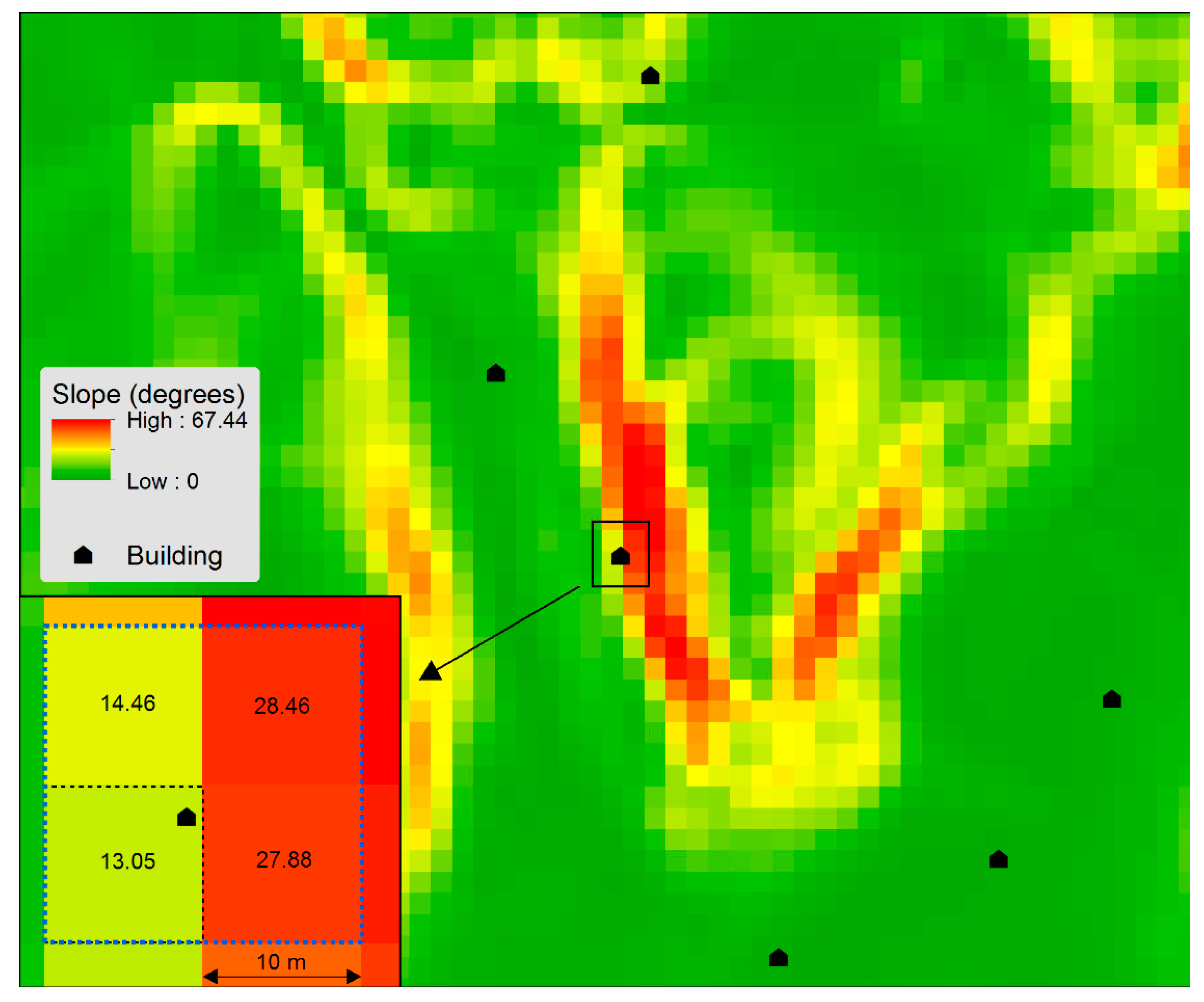
Figure 2.
Scores (upper plot) and loadings (lower plot) computed from PLS.


Table 1.
Variables included in the PLS-analysis.
| Group | No | Abbrev. | Parameter | Flooded (F) Addresses | Random (R) Addresses | BCP = Building Central Point Comments | ||
|---|---|---|---|---|---|---|---|---|
| Aver | (SD) | Aver | (SD) | |||||
| Distance | 1 | d_C | Distance to coast | 627 | (415) | 639 | (471) | Distance from BCP to coast (m) |
| Distance | 2 | d_z1 | elevation_1m area | 14.95 | (11) | 22.61 | (14) | Elevation extracted from 1 m resolution DEM at location of BCP |
| Distance | 3 | d_z10 | elevation_10m area | 15.34 | (11) | 22.60 | (14) | As above, 10 m resolution |
| Distance | 4 | d_z50 | elevation_50m area | 15.80 | (11) | 22.57 | (14) | As above, 50 m resolution |
| Slope | 5 | sl_1 | slope_1m | 2.6 | (3,1) | 5.1 | (4,6) | Mean slope extracted from 1 m resolution DEM at location of BCP |
| Slope | 6 | sl_10 | slope_10m | 2.2 | (2,2) | 5.3 | (4,2) | As above, 10 m resolution |
| Slope | 7 | sl_50 | slope_50m | 2.3 | (2,1) | 3.9 | (2,9) | As above, 50 m resolution |
| Slope | 8 | sl_r100 | Slope_r100 | 5.9 | (3,8) | 7.7 | (3,9) | Mean slope extracted from 100 m radius at location of BCP |
| Slope | 9 | sl_1_ip | slope_1m interpolated | 2.6 | (3,1) | 5.1 | (4,6) | Mean slope extracted from 1 m resolution DEM at location of BCP and its 8 first neighbors |
| Slope | 10 | sl_10_ip | slope_10m interpolated | 2.2 | (2,3) | 5.5 | (4,2) | As above, 10 m resolution |
| Slope | 11 | sl_50_ip | slope_50m interpolated | 2.4 | (2,0) | 3.9 | (2,6) | As above, 50 m resolution |
| Area | 12 | a_Up | UpSlope area | 18,047 | (4934) | 13,171 | (5381) | Area at higher ground than BCP within 100 m radius |
| Area | 13 | a_Up_ro | UpSlope impervious area | 1761 | (941) | 999 | (840) | Roads(impervious) at higher ground than BCP within 100 m radius |
| Area | 14 | a_RUp_ro | Rate UpSlope impervious area | 0.10 | 0.05 | 0.07 | 0,05 | Ratio No. 13/No. 12 |
| Area | 15 | a_DS | Cells downstream | 13,382 | (4957) | 18,183 | (5407) | Area at lower ground than BCP within 100 m radius |
| Area | 16 | a_US | Cells upstream | 17,986 | (4957) | 13,186 | (5407) | Area at higher ground than BCP within 100 m radius |
| Area | 17 | a_US_im | Cells impervious | 15,880 | (5168) | 11,167 | (5528) | Area of imperm surfaces at higher ground than BCP within 100 m radius |
| Area | 18 | a_US_pe | Cells pervious | 2106 | (3158) | 1966 | (3761) | Area of perm. surfaces at higher ground than BCP within 100 m radius |
| Area | 19 | a_RUS_im | Rate Cells impervious | 0.89 | (0,2) | 0.86 | 0,24 | Ratio No. 17/ No. 16 |
| Curvature | 20 | c_pr1 | curvature profile 1 m | 0.16 | (1,7) | −0.17 | (3,0) | Profile curvature extracted from 1 m resolution DEM at location of BCP |
| Curvature | 21 | c_pr10 | curvature profile 10 m | 0.07 | (0,3) | 0.04 | (0,6) | As above, 10 m resolution |
| Curvature | 22 | c_pr50 | curvature profile 50 m | 0.07 | (0,1) | −0.01 | (0,1) | As above, 50 m resolution |
| Curvature | 23 | c_pr1_ip | curvature profile 1 m interpolated | 0.14 | (1,2) | −0.13 | (2,1) | Weighted mean profile curvature extracted from 1 m resolution DEM based on four closest pixels to location of BCP |
| Curvature | 24 | c_pr10_ip | curvature profile 10 m interpolated | 0.08 | (0,2) | 0.03 | (0,6) | As above, 10 m resolution |
| Curvature | 25 | c_pr50_ip | curvature profile 50 m interpolated | 0.06 | (0,1) | 0.00 | (0,1) | As above, 50 m resolution |
| Curvature | 26 | c_pl1 | curvature plan 1 m | 0.18 | (1,9) | 0.02 | (1,8) | Plan curvature extracted from 1 m resolution DEM at location of BCP |
| Curvature | 27 | c_pl10 | curvature plan 10 m | −0.02 | (0,2) | 0.06 | (0,3) | As above, 10 m resolution |
| Curvature | 28 | c_pl50 | curvature plan 50 m | −0.02 | (0,1) | 0.03 | (0,1) | As above, 50 m resolution |
| Curvature | 29 | c_pl1_ip | curvature plan 1 m interpolated | 0.14 | (1,4) | 0.05 | (1,5) | Weighted mean plan curvature extracted from 1 m resolution DEM based on four closest pixels to location of BCP |
| Curvature | 30 | c_pl10_ip | curvature plan 10 m interpolated | −0.02 | (0,1) | 0.06 | (0,3) | As above, 10 m resolution |
| Curvature | 31 | c_pl50_ip | curvature plan 50 m interpolated | −0.02 | (0,0) | 0.02 | (0,1) | As above, 50 m resolution |
| Sewer | 32 | se_C | Combined sewer mains (rate) | 66% | 46% | Rate combined system (category var) | ||
| Sewer | 33 | se_S | Separate sewer mains (rate) | 34% | 54% | Rate separate system (category var) | ||
| Sewer | 34 | se_D | Diameter pipe(mm) | 369 | (225) | 269 | (134) | Diameter of nearest sewer pipe |
| Sewer | 35 | se_Y | Year of constructed pipe | 1972 | (26,2) | 1974 | (23,0) | Year of construction for the nearest sewer mains |
| Sewer | 36 | se_HorD | Horizontal dist to sewer | 20.9 | (9,9) | 29.2 | (23,3) | Horizontal distance from BCP to the nearest sewer |
| Sewer | 37 | se_V>2 | Vertical dist to sewer >2 m | 0% | 16% | Vertical distance from BCP to sewer mains >2 m (category variable) | ||
| Sewer | 38 | se_V<2 | Vertical dist to sewer <2 m | 100% | 84% | Vertical distance from BCP to sewer mains<2 m (category variable) | ||
© 2017 by the authors. Licensee MDPI, Basel, Switzerland. This article is an open access article distributed under the terms and conditions of the Creative Commons Attribution (CC BY) license (http://creativecommons.org/licenses/by/4.0/).
Share and Cite
MDPI and ACS Style
Torgersen, G.; Rød, J.K.; Kvaal, K.; Bjerkholt, J.T.; Lindholm, O.G. Evaluating Flood Exposure for Properties in Urban Areas Using a Multivariate Modelling Technique. Water 2017, 9, 318. https://doi.org/10.3390/w9050318
AMA Style
Torgersen G, Rød JK, Kvaal K, Bjerkholt JT, Lindholm OG. Evaluating Flood Exposure for Properties in Urban Areas Using a Multivariate Modelling Technique. Water. 2017; 9(5):318. https://doi.org/10.3390/w9050318
Chicago/Turabian StyleTorgersen, Geir, Jan Ketil Rød, Knut Kvaal, Jarle T. Bjerkholt, and Oddvar G. Lindholm. 2017. "Evaluating Flood Exposure for Properties in Urban Areas Using a Multivariate Modelling Technique" Water 9, no. 5: 318. https://doi.org/10.3390/w9050318
Note that from the first issue of 2016, this journal uses article numbers instead of page numbers. See further details here.