Article

Exploring Streamwater Mixing Dynamics via Handheld Thermal Infrared Imagery

1
Catchment and Eco-Hydrology Group, Department of Environmental Research and Innovation, Luxembourg Institute of Science and Technology, 41 rue du Brill, Belvaux L-4422, Luxembourg
2
Hydrology and Quantitative Water Management Group, Wageningen University & Research, Wageningen 6708 PB, The Netherlands
3
Civil, Environmental and Mining Engineering, University of Western Australia, Perth, WA 6009, Australia
4
Veterinary and Life Sciences, Murdoch University, Perth, WA 6009, Australia
*
Author to whom correspondence should be addressed.
Water 2017, 9(5), 358; https://doi.org/10.3390/w9050358
Submission received: 7 March 2017 / Revised: 12 May 2017 / Accepted: 15 May 2017 / Published: 19 May 2017
(This article belongs to the Special Issue New Developments in Methods for Hydrological Process Understanding)

Abstract

:
Stream confluences are important hotspots of aquatic ecological processes. Water mixing dynamics at stream confluences influence physio-chemical characteristics of the stream as well as sediment mobilisation and pollutant dispersal. In this study, we investigated the potential for handheld thermal infrared (TIR) imagery to provide rapid information on stream water mixing dynamics at small scales. In-situ visualisation of water mixing patterns can help reduce analytical errors related to stream water sampling locations and improve our understanding of how confluences and tributaries influence aquatic ecological communities. We compared TIR-inferred stream temperature distributions with water electrical conductivity and temperature (measured with a submerged probe) data from cross-channel transects. We show that the use of a portable TIR camera can enhance the visualisation of mixing dynamics taking place at stream confluences, identify the location of the mixing front between two different water sources and the degree of mixing. Interpretation of handheld TIR observations also provided information on how stream morphology and discharge can influence mixing dynamics in small streams. Overall, this study shows that TIR imagery is a valuable support technique for eco-hydrological investigation at small stream confluences.

1. Introduction

Water flow fields in rivers control the dispersal of solutes and pollutants, as well as the mobilisation of sediments—eventually influencing habitat variability and stream biodiversity [1,2,3,4]. Furthermore, proper consideration of water mixing dynamics near the surface is key for reducing errors in water sampling protocols and tracer experiments in small catchments and/or near stream confluences [5,6]. Complete mixing of different water end-members stands as a fundamental assumption in classic hydrograph separation [7]. Likewise, it is a prerequisite for hydrometric measurements such as salt dilution gauging [8]. Streamwater samples can be strongly influenced by lateral inflows from soil or groundwater [9,10,11].
In experimental hydrology, stream temperature is widely recognised as an effective indicator of hydrological connectivity, water flow paths and hyporheic exchanges [12,13,14]. In rivers, temperature exerts an important control on physiochemical characteristics of water [15] and it is a driver of numerous biological processes, controlling the structure of ecological communities and habitat complexity [16,17]. Approaches for measuring stream water temperature cover a wide range of methods including temperature loggers and thermometers [18,19,20], fiber-optic distributed temperature sensing (FO-DTS) [21,22] and thermal infrared (TIR) cameras [23,24,25].
Among these measurement tools, TIR cameras are particularly suitable for the collection of temperature data at multiple spatial and temporal scales with high resolution [26,27], overcoming the limitations of discrete measurements. To date, airborne and ground-based TIR imagery have been successfully used to describe longitudinal profiles of river temperature [27,28,29,30], to provide information on soil moisture and surface saturation patterns [31,32], to detect ground water exfiltration along the hillslope-riparian-stream continuum and inferring connectivity dynamics of water exfiltrating to the stream [33,34,35,36,37]. Furthermore, information obtained through TIR imagery has been used as a data source for hydrological model validation [32,38]. Thus far, the potential for handheld TIR imagery to assess water mixing dynamics in small streams has not been fully assessed [23,25,35,39], with the vast majority of the studies relying on airborne TIR observations or reporting only some marginal observations specifically on water mixing. Most studies on water mixing at small scales rely on measurements of water temperature, electrical conductivity and flow velocities with probes placed at different depths in the water column [40,41,42,43]. Ground-based TIR imagery could be a potentially useful method for supporting in-situ selections of representative sampling locations—thereby reducing uncertainties inherent to fundamental mixing assumptions or water quality monitoring campaigns [6,44].
In this paper we investigate the potential for handheld TIR imagery to provide instantaneous mapping of stream water mixing patterns at or near the water surface. We test if thermal patterns observed at the stream surface adequately represent water mixing dynamics. More specifically, we investigate if mixing length, location and width of the mixing front and gradients of solute concentrations between different sources can be inferred from ground-based TIR images under low flow conditions in small streams.
First, we compare information extracted from the TIR observations with data of water electrical conductivity and temperature obtained with a submerged multi-probe from cross-channel transects, located downstream of two confluences in a natural and an urban setting. Next, we analyse and discuss the results to provide an overview of the possible advantages and disadvantages of the hand-held TIR technology.

2. Materials and Methods
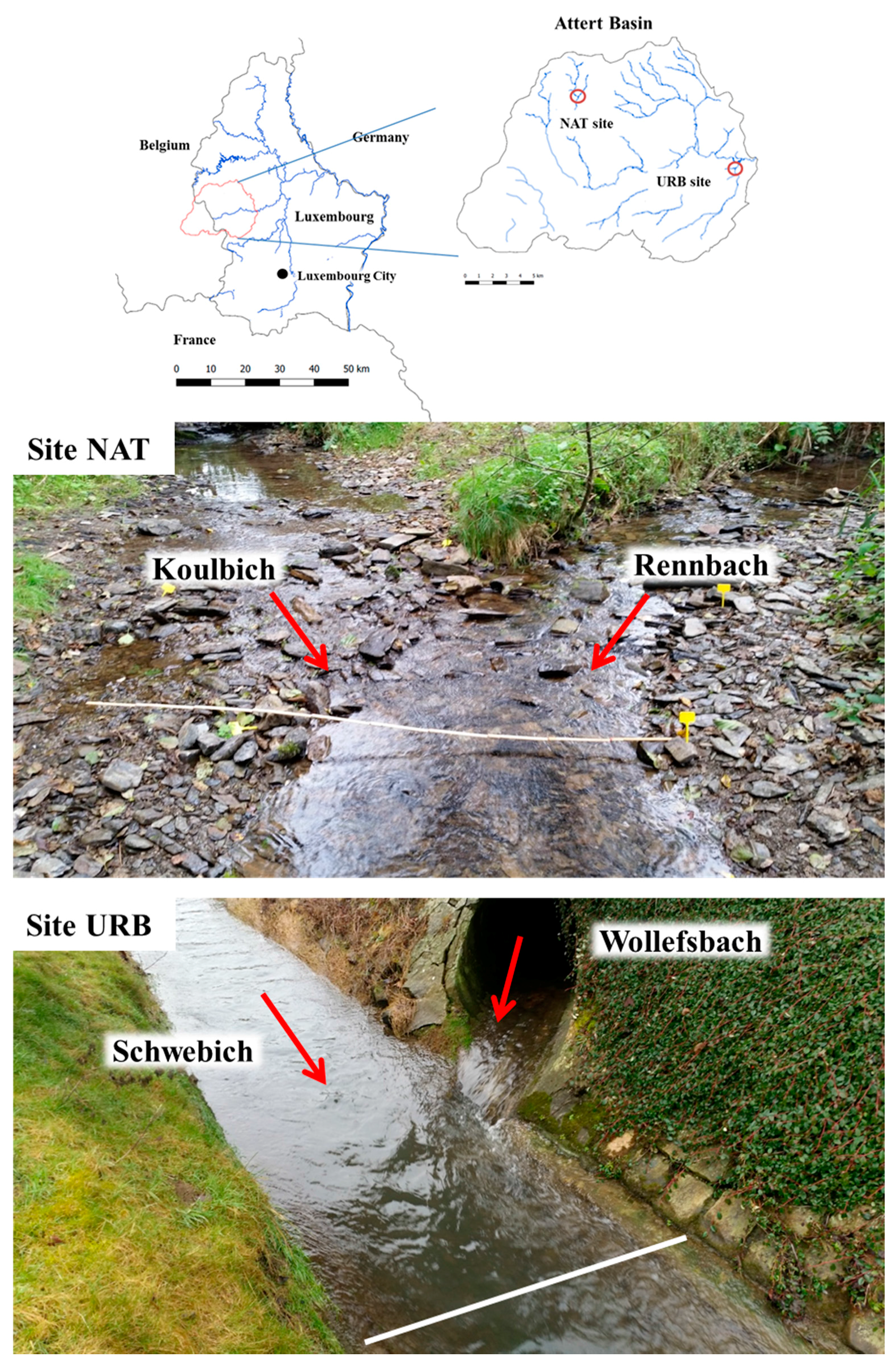
2.1. Study Sites

We selected two stream confluences in the Attert River basin (247.03 km2—located in the North-West of the Grand Duchy of Luxembourg) for our investigations (Figure 1).
The confluence of the Koulbich and the Rennbach (natural stream confluence [NAT]—49°48′42.4″ N, 5°48′49.8″ E) creeks corresponds to a symmetrical headwater junction located in a natural area—mostly dominated by forests further upstream. At the confluence, the two creeks flow through meadows directly on the schistose bedrock, characteristic of the northern part of the Attert River basin. Together with the coarse bedload sediment, this bedrock confers a highly irregular bed profile to the creeks.
The confluence of the Schwebich and the Wollefsbach (urban stream confluence [URB]—49°45′51.3″ N, 5°58′36.9″ E) creeks corresponds to a channelized asymmetrical junction flowing through a small village. No accumulated material is present in the proximity of the junction and the stream bed has a regular trapezoidal cross section.
In both sites we observed a difference in water depth of the two streams before the junction. The Rennbach (mid-point depth: ~5–8 cm) and the Schwebich (mid-point depth: ~20–22 cm) were deeper than the Koulbich (mid-point depth: ~2–5 cm) and the Wollefsbach (mid-point depth: ~5 cm), respectively.

2.2. Field Measurements

During storm events, surface roughness, deeper water columns as well as stream temperature homogenisation due to precipitation tend to influence the applicability of remotely sensed data [27,45]. Consequently, because we are making these measurements for the first time we concentrated on winter low flows, when these disturbances were small and temperature contrasts more pronounced. In the investigated catchments, these particular flow conditions are equivalent to summer low flow.
We measured discharge, water electrical conductivity (EC) and water temperature on four days (21 and 28 September, 17 November and 1 December 2016) at the NAT site and on two days (2 and 9 February 2017) at the URB site. Although we had carried out a significantly larger number of TIR observations at the two sites (on the 21 and 27 October 2016 and 10 and 24 November 2016 at the NAT site and on the 17 and 27 January 2017 at the URB site), on the aforementioned six dates the temperature contrast between the tributaries was found to be particularly suitable for our TIR observations.
Water EC and temperature were measured using a conductivity meter WTW Multi 3420 equipped with a TetraCon 925 probe (Xylem Analytics, Weilheim, Germany), providing a conductivity resolution of 0.1 µS/cm from 0 to 199 µS/cm and 1 µS/cm from 200 to 1999 µS/cm; and a temperature resolution of 0.1 from −5 to 100 °C. Measurements were taken every 5 or 10 cm along three cross-channel transects, at 1.5 m (transect A), 3 m (transect B) and 9 m (transect C) downstream of the junctions. Measurements were made at the stream bottom and, when the water was deep enough (i.e., ≥~8 cm due to the probe’s sensor length), also near the surface. Streambed cross-sectional depth profiles were obtained for the transect locations at both sites.
We measured stream discharge up- and downstream of the junction using the salt dilution method at the NAT site and from stream gauges at the URB site (estimated from water level data via a rating curve). Air temperature was obtained from meteorological stations operated by the Ministry of Agriculture and located in the vicinity of our experimental sites (~2 km between the meteorological station and the NAT site and ~1 km between the meteorological station and the URB site).

2.3. TIR Image Acquisition

We collected TIR images from both study sites using a handheld FLIR TIR camera (FLIR T640, FLIR Systems, Wilsonville, OR, USA). With this technology, the radiation emitted by an object’s surface (i.e., the first 0.1 mm of the water surface in this study) can be quantified and converted into visible temperature patterns in thermal images. The camera used produces thermal images of 640 × 480 pixels over a spectral range of 7.5 to 14 µm. Its temperature range is −40 °C to 2000 °C, with a thermal sensitivity of <0.035 °C at 30 °C.
Before acquiring the images it is necessary to provide the camera with information about object emissivity “ε” (usually set between 0.95 and 0.97 for freshwater), atmospheric temperature, air humidity, object’s distance from the camera and reflected ambient temperature [46].
The employed camera automatically corrects the detected temperature for the aforementioned parameters.
TIR images were taken in each transect simultaneously to the other measurements (Figure 2A). The images were taken by positioning the handheld camera perpendicular to the stream section under study and trying to cover the widest possible width with a single image. Since our purpose was to extract temperature cross-sectional distributions from the thermal images, we avoided using the panoramic picture mode, where shifts in absolute temperature can occur between contiguous images as a product of the camera’s non-uniformity correction [27]. Moreover, both confluences were chosen in cleared areas in order to avoid tree shading effects which can influence the temperature detection.
In order to understand if distance to complete mixing (i.e., the distance downstream from the confluence where no differences in water EC could be detected along a stream cross-section and in the water column) can be assessed from TIR in-situ observations, we walked downstream from the confluences during the different sampling dates, monitoring the streams with the TIR camera until no difference in temperature could be detected between the stream banks. Ground measurements of water EC and water temperature were then carried out at the same distance downstream from the confluence where no temperature difference was detectable between the stream banks using the TIR camera.
A summary of air temperature values (daily average), stream discharge, relative difference in temperature and EC between the tributaries, distance to complete mixing for the different sampling days and the stream temperature at that location are listed in Table 1. Information on the sub-basin area at the two confluences, cross-section geometry at the transects, stream bed roughness and tracer velocities are also reported. Examples of stream depth cross-sectional profiles are shown in Figure 2B (the two examples are representative of the depth profiles along the transects in the NAT site and the URB site).

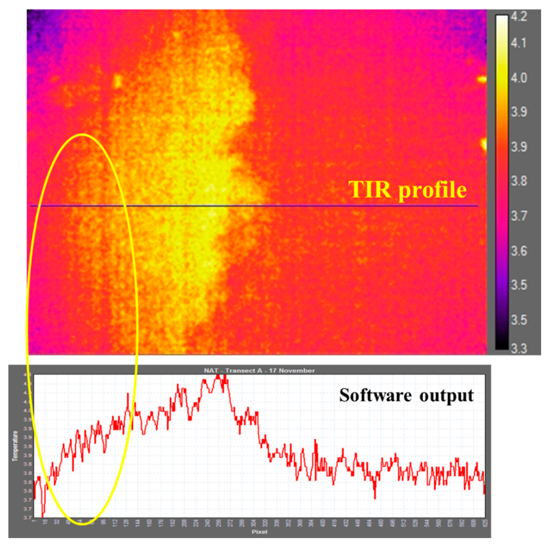
2.4. Data Processing and Analyses

Temperature cross-sectional distributions were extracted from the thermal images using the FLIR ResearchIR software (Figure 3). We applied cubic spline smoothing [48] on EC, temperature and TIR-inferred temperature data collected along the different transects. We tested the correlation between the original data and the smoothed distributions through correlation analysis and analysis of the residuals. This approach allowed us to highlight curve trends and simplify the comparison between the information from the EC and temperature measurements and the TIR-inferred temperature.
The inflection point on the smoothed curves indicates the point along the transects where the main shift between two different water sources occurs (mixing front). Analogously, we use the width of the slope surrounding the inflection point as an indicator of the portion of the transect where the mixing preferentially occurs (mixing width). This portion is where stream water EC and temperature start to show differences from the EC and temperature of the two original sources.
We defined the main slope of the curve as the section with a gradient of at least 50% of the curve’s maximum gradient. We choose this threshold to account for the inherent variability of the curves’ profiles. The main slope and the inflection point were estimated from the first and second derivative, respectively, which were calculated using a finite difference approximation of the smoothed curves.
To test if gradients of solute concentration between different sources can be inferred from ground-based TIR images, we quantified the relation between the curves of EC, temperature and TIR temperature using correlation analyses. Then we compared the location of the mixing front and the mixing width inferred from all the curves (along all the cross-sectional transects for each sampling date at both study sites).
The data smoothing and the correlation analyses were carried out in R 3.2.2 [49].

3. Results and Discussion

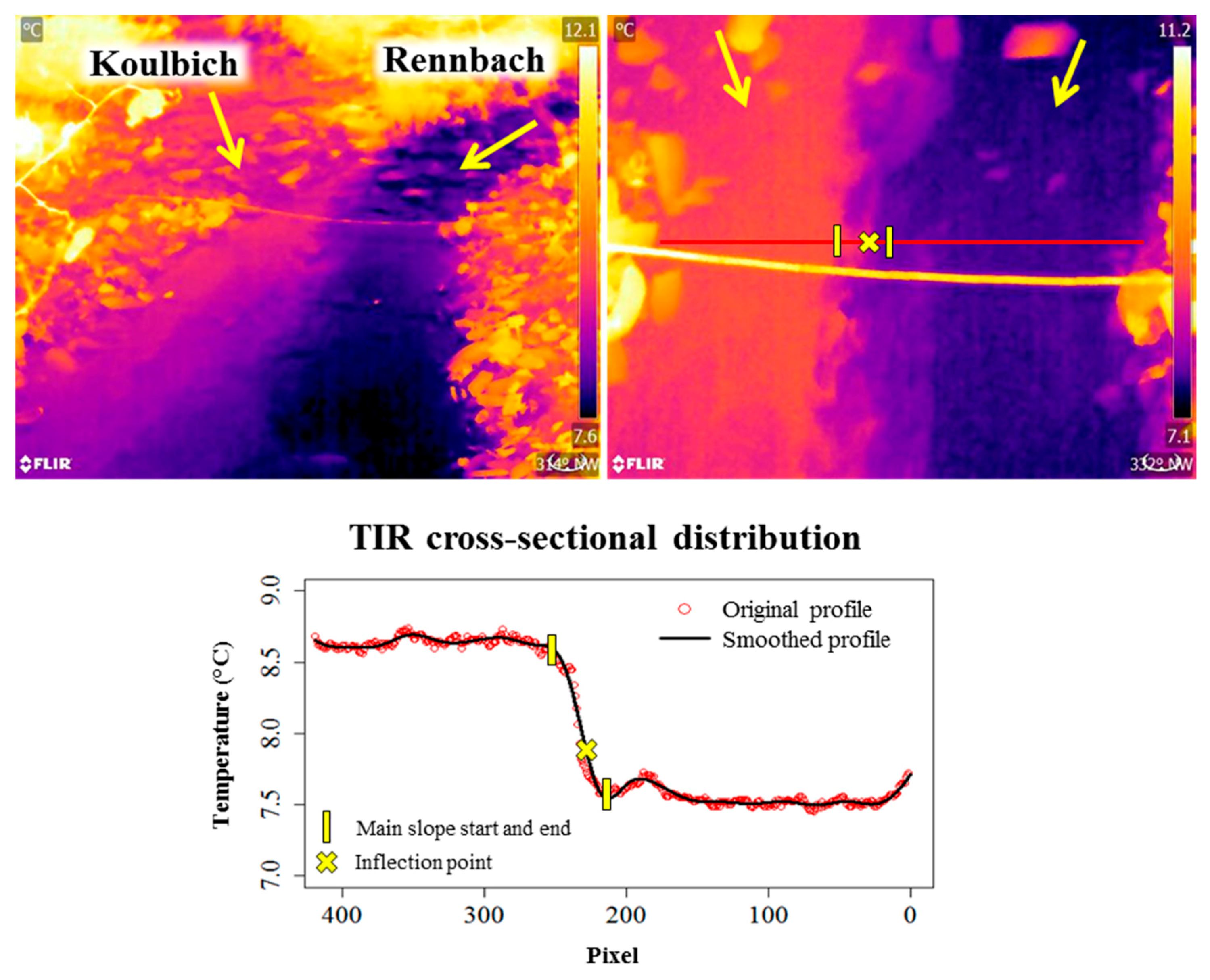
3.1. Consistency between Temperatures “Sensed” with the TIR Camera and a Submerged Probe

Stream water temperatures detected by the TIR camera did not exactly match the temperature probe measurements. The temperature difference ranged between 1 and 2.8 °C on days of higher air temperature (21 and 28 September) and between 3.8 and 5.4 °C on days with lower air temperature (17 November, 1 December and 2 and 9 February). We identified several potential reasons that might cause these discrepancies in temperature measurements: (1) while the camera is only ‘sensing’ long-wave radiation emitted by the surface of the water column (0.1 mm depth), the probes need to be totally submerged and therefore represent temperature over a depth of 4 cm; (2) the camera hardware appeared to be sensitive to external temperatures—the difference in temperatures ‘sensed’ by the TIR imagery and measured with the submerged probe was significantly enhanced during days with low air temperature.
Despite the aforementioned differences between temperatures measured with the TIR camera and the probe, the relative temperature difference determined between the tributaries was identical for both devices, with a maximum difference of 0.8 °C (again, occurring on the day with colder air temperature—1 December).

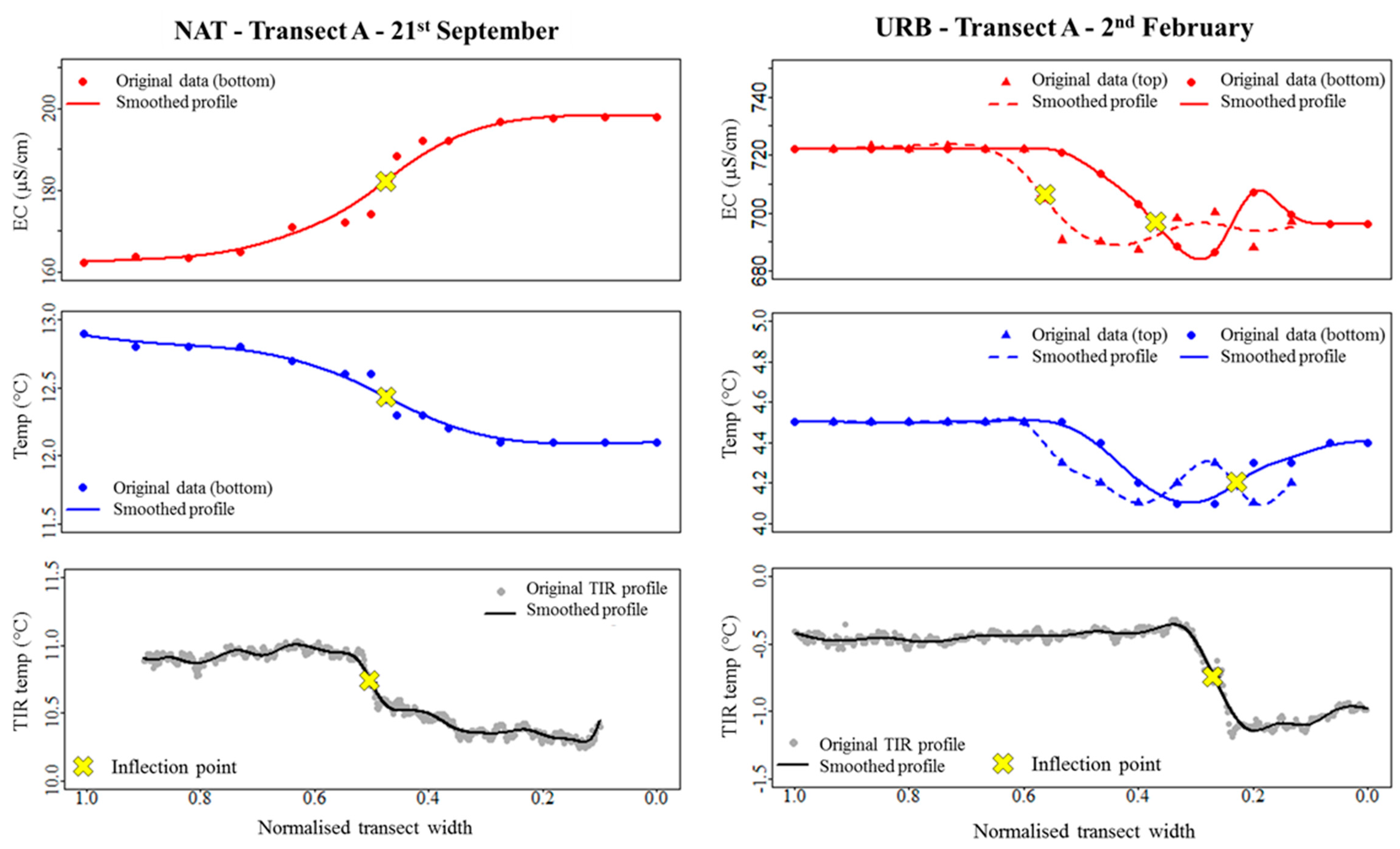
3.2. Inferring Complete Mixing from TIR Stream Observations

The environmental parameters measured during the different sampling days at the two sites (summarised in Table 1) helped us to partition our observations into two different hydrological conditions. During the first two sampling dates for the NAT site (the 21 and 28 September 2016) and the first sampling date for the URB site (the 2 February 2017) we observed higher air and stream temperature, together with higher temperature contrasts between the tributaries and lower stream discharge than during the other sampling dates (17 November and the 1 December 2016 for the NAT site and the 9 February for the URB site). At the NAT site the length to complete mixing increased with increasing stream discharge, while it decreased with increased stream discharge at URB. Nevertheless, the distance to complete mixing can be influenced by a number of factors, such as stream discharge, stream bed morphology and particular features as riffles and pools and water density [43,50].
Information on complete mixing inferred from monitoring the stream with the TIR camera was found to be discordant with the information from the water EC values measured in the stream. In most cases, homogeneities in temperature were detected by the TIR camera and the temperature probe before EC complete mixing was reached. This discordance can be due to the different magnitude of in stream EC and temperature differences between the two tributaries (EC relative difference between the streams was always higher than the difference in temperature) combined with the measurement resolution of the probe and the TIR camera. In our case, we could obtain finer measurements of stream water EC than of temperature both from TIR observations and measured with the probe. Ultimately, this may jeopardize the detection of temperature differences at downstream locations where differences in EC would still be measurable. Indeed, the best match in the measurements of TIR-inferred temperature and water EC was observed in two cases: the 28 of September in the NAT site and the 2 of February for the URB site. During those dates we recorded the highest temperature contrast between the tributaries at both sites and a nearly total absence of waves on the water surface. The lower emissivity that characterizes rippled water surfaces influences the temperature measurements made with a TIR camera [23,24]. Even when there are strong temperature contrasts between two water sources, surface roughness may complicate the in-situ interpretation of TIR images and ultimately the inference of reliable distances to complete mixing.

3.3. Comparison between Stream EC and Temperature Inferred from Submerged Probe and TIR-Inferred Water Surface Temperature

The correlation between the original measured data and the curves obtained via smoothing techniques was generally good (Pearson’s R2 > 0.83). Surface water TIR distributions showed a good correlation with the measurements of water EC and temperature (Pearson’s R2 > 0.85) in particular at the NAT site along the transect A (Figure 4) and B, located closer to the junction. At the URB site, the best correlation was found during the first sampling day, especially for transect C, located furthest from the junction. When poor correlation occurred, it was often associated with a combination between poor temperature contrast and surface roughness (mainly related to the presence of surface waves). Nevertheless, in the NAT site, transect C was the one placed in the cross-section presenting the highest superficial roughness (mainly due to the streambed morphology at that location), while in the URB site, the majority of the roughness was located closer to the junction, caused by the presence of the junction itself (Figure 4). Moreover, at transect A (URB) we observed during both sampling days the highest vertical differences in EC and temperature measurements between the bottom and the surface of the water column. The water from the shallowest tributary (Wollefsbach) tended to flow on top of the deepest tributary (Schwebich), especially during the day of lower discharge (2 February) [39]. Despite flow pattern complexities at this location, the TIR cross-sectional distribution showed modest correlation with the distribution of EC and temperature measured at the surface (R2 = 0.70 and R2 = 0.59, respectively).
Other sources of poor correlation were to attribute to the presence of an “aura” in some TIR images surrounding the digital image (probably due to sensor noise), which noticeably influenced the extraction of the TIR data for the images collected on the 17 November in the NAT site (Figure 5) and to reflection from the river banks (which occurred in particular on the 9 February at the URB site). In this case, cross-sectional distributions affected by these sources of error have been corrected by excluding the area influenced by the error (usually places at the extremities of the distribution).
Table 2 shows the absolute distance (in cm) between the location of the mixing front calculated from the TIR cross-sectional distributions and the other parameters (water EC and temperature measured at the streambed and surface) for both dates along all transects at each site. Overall, 71% of the times the TIR observations placed the mixing front at less than or equal to 30 cm from the location inferred through water EC or temperature. In 43% of these cases the distance was less than 10 cm. Differences higher than 30 cm have been detected especially during days when the two tributaries had the lower relative difference in temperature and the higher relative difference in EC (i.e., 17 November at the NAT site and the 9 February at the URB site). As mentioned earlier, the resolution of the different instruments could affect inter-comparison of the different measurements. For example, we expected the information provided by the camera to have a higher similarity (in terms of correlation and mixing front location) to water temperature (measured with the probe) than to EC. Nevertheless, in some cases the smoothing technique (and the consequent calculation of inflection point and main slope of the curve) did not work properly on the temperature probe data. This may be due to the fact that, when the temperature difference between the tributaries is small, the resolution of the probe (0.1 °C) is too low causing the smoothing to fail (regardless of the number of original data points considered in the analysis).

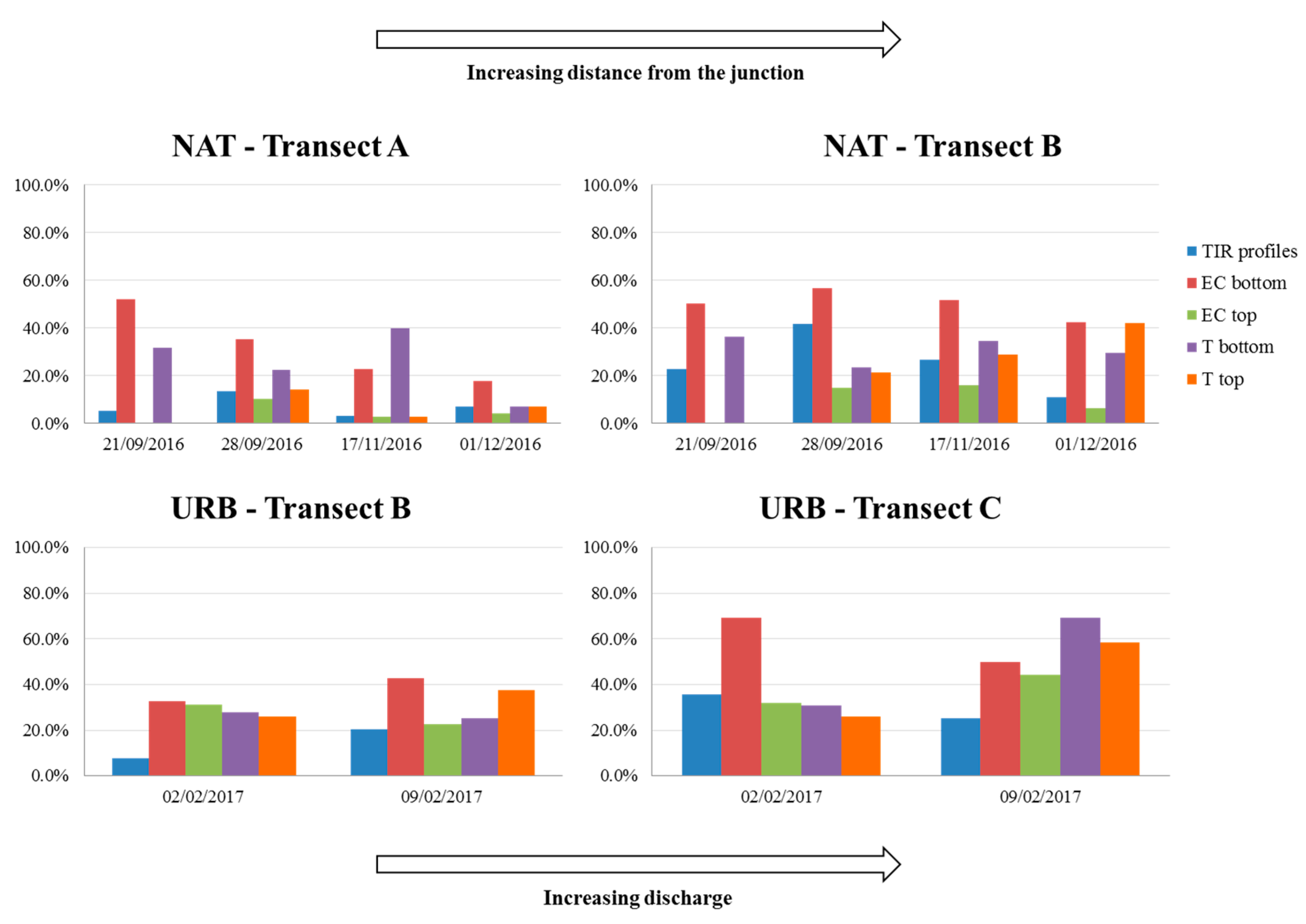
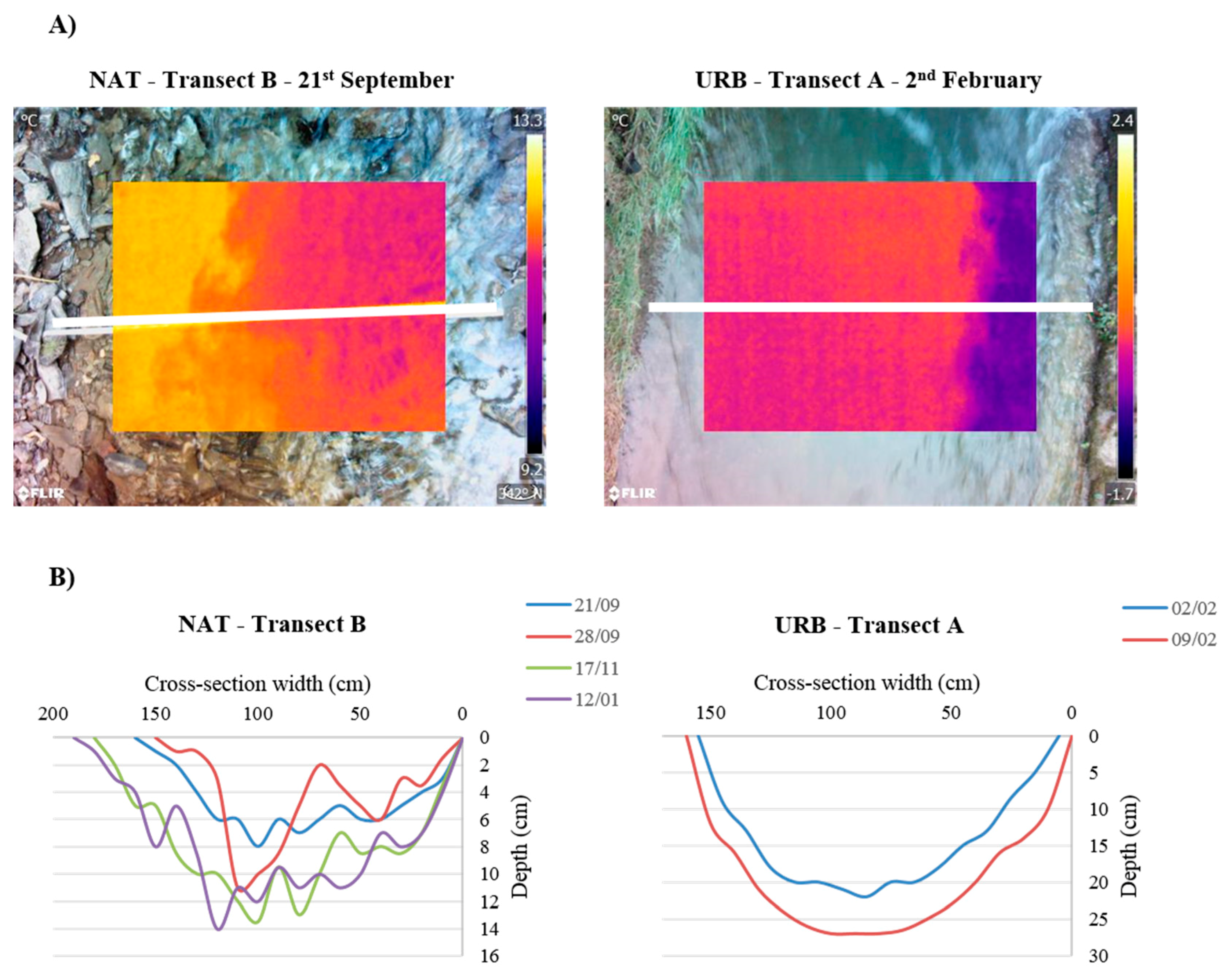
3.4. Influence of Discharge and Streambed Morphology on Location of the Mixing Front and Mixing Width

For both study sites, we did not detect a clear relationship between the mixing width (i.e., the portion along the transects where mixing preferentially occurs, expressed here as a percentage of the total transect width) and stream discharge (Figure 6). For this analysis, we accounted only for cases where a good correlation between the TIR-inferred temperature distribution and water EC and temperature had been observed. In the NAT site, the mixing width generally increased with increasing distance from the stream junctions, while in the URB site this trend was less evident (Figure 6). For both sites, the mixing width retrieved from the TIR distributions was usually shorter than the one inferred from water EC and temperature, especially when measured at the stream bottom. Mixing dynamics taking place in the water column could not unequivocally be translated into clear thermal patterns near the water surface. Indeed, the TIR-inferred mixing widths turned out to be more similar to those calculated from water EC and temperature distributions measured near the stream surface.
Transect length and stream water depth increased with rising discharge at both sites. However, regardless of discharge values, the mixing front was located mainly on the right side of the stream (looking upstream) in both study sites. At the NAT site, stream bed morphology may control the location of mixing fronts. For example, the right tributary (Rennbach) and the right side of the stream after the junction were found to be deeper than the left side. In this case, water from the shallower tributary could tend to flow on top of water flowing from the deeper one [40]. Eventually this may result in a shift of mixing areas towards the right side of the stream, although the confluence has a symmetrical shape. In the URB site, characterised by a paved stream bed, the predominant right-side location of the mixing front may reflect the hydrological conditions of the stream together with the considerable depth difference between the two tributaries and their junction angle.

4. Conclusions

In two contrasting experimental sites, we have documented how water surface temperature data obtained from handheld TIR cameras compares to in-stream EC and temperature data. A common feature to all our TIR observations is that cross-sectional variability in surface temperature reflects in-stream temperature and chemistry variability. This relationship is even stronger when temperature contrasts are high between two tributaries and superficial roughness is low at the observed cross-section.
We have shown that ground-based TIR imagery provides valuable information for rapid in-situ visualisation of water mixing and mixing dynamics at the scales represented in this study. In particular, we were able to identify the position of the mixing front along the stream cross-sections and the distance to complete mixing, especially when the TIR images were acquired under favourable conditions.
More research is needed before one can unequivocally determine distance to complete mixing through TIR imagery. Future work should focus on the effects of low temperature contrasts and water surface roughness, which can directly influence temperature measured by TIR cameras. Additional investigations may also explore further the potential for TIR observations to characterise streambed morphology and discharge controls on water mixing dynamics.
Stream confluences represent important eco-hydrological hotspots, where water with potentially different physio-chemical characteristics mix along an interface [51]. Our methodology using ground-based TIR imagery could be a valuable support tool for eco-hydrological studies interested in identification of changing environmental conditions around confluences [3]. The use of a handheld TIR camera allows visualisation of this mixing process as it evolves from clear separation of tributary sources at the confluence to complete mixing further downstream.
Handheld TIR approach as presented in this study could aid optimization of water sampling procedures for qualitative and quantitative hydrological analyses at the proximity of confluences, by assisting in the determination of in-stream representative sampling locations [6,44]. Handheld TIR observations of water mixing could also provide insights on the dispersal dynamics of suspended sediments and dissolved substances at confluences [50,52].
In order to improve validation of the method, we are now undertaking additional work with in-situ TIR cameras to improve the handheld TIR imagery approach under changing hydrological conditions.

Acknowledgments

This project has been funded by the European Union’s Seventh Framework Program for research, technological development and demonstration under grant agreement No. 607150 (FP7−PEOPLE−2013−ITN—INTERFACES—Ecohydrological interfaces as critical hotspots for transformations of ecosystem exchange fluxes and bio-geochemical cycling) and by the Luxembourg National Research Fund FNR MOBILITY/16/11256906—SOLACE. We would like to thank the ASTA (Administration des services techniques de l’agriculture, Luxembourg) for supplying air temperature data from the meteorological stations of Useldange and Roodt. We would like to thank Barbara Glaser and Marco Coccon for the helpful discussions. We would also like to thank two anonymous reviewers and the Academic Editor for their thoughtful comments.

Author Contributions

Marta Antonelli, Julian Klaus, Keith Smettem and Laurent Pfister conceived and design of the study; Marta Antonelli performed the experiments and analyzed the data; Marta Antonelli, Julian Klaus, Keith Smettem, Adriaan J. Teuling and Laurent Pfister contributed to the interpretation of the results and the preparation of the manuscript.

Conflicts of Interest

The authors declare no conflict of interest.

References

  1. Power, M.E.; Dietrich, W.E. Food webs in river networks. Ecol. Res. 2002, 17, 451–471. [Google Scholar] [CrossRef]
  2. Kiffney, P.M.; Greene, C.M.; Hall, J.E.; Davies, J.R. Tributary streams create spatial discontinuities in habitat, biological productivity, and diversity in mainstem rivers. Can. J. Fish. Aquat. Sci. 2006, 63, 2518–2530. [Google Scholar] [CrossRef]
  3. Rice, S.; Kiffney, P.; Greene, C.; Pess, G.R. The ecological importance of tributaries and confluences. In River Confluences, Tributaries and the Fluvial Network; Rice, S.P., Roy, A.G., Rhoads, B.L., Eds.; John Wiley & Sons, Ltd.: Chichester, UK, 2008; pp. 209–237. [Google Scholar] [CrossRef]
  4. Rice, P.S. Tributary connectivity, confluence aggradation and network biodiversity. Geomorphology 2017, 277, 6–16. [Google Scholar] [CrossRef]
  5. Sanders, T.G.; Adrian, D.D.; Joyce, M.J. Mixing Length for Representative Water Quality Sampling. J. Water Pollut. Control Fed. 1977, 49, 2467–2478. [Google Scholar]
  6. Sanders, T.G. Representative sampling location criterion for rivers. Water SA 1982, 8, 169–172. [Google Scholar]
  7. Klaus, J.; McDonnell, J.J. Hydrograph separation using stable isotopes: Review and evaluation. J. Hydrol. 2013, 505, 47–64. [Google Scholar] [CrossRef]
  8. Hongve, D. A revised procedure for discharge measurement by means of the salt dilution method. Hydrol. Process. 1987, 1, 267–270. [Google Scholar] [CrossRef]
  9. Kemp, M.J.; Dodds, W.K. Spatial and temporal patterns of nitrogen concentrations in pristine and agriculturally-influenced prairie streams. Biogeochemistry 2001, 53, 125–141. [Google Scholar] [CrossRef]
  10. Soulsby, C.; Malcolm, I.A.; Youngson, A.F.; Tetzlaff, D.; Gibbins, C.N.; Hannah, D.M. Groundwater-surface water interactions in upland Scottish rivers: Hydrological, hydrochemical and ecological implications. Scott. J. Geol. 2005, 41, 39–49. [Google Scholar] [CrossRef]
  11. Rademacher, L.K.; Clark, J.F.; Clow, D.W.; Hudson, G.B. Old groundwater influence on stream hydrochemistry and catchment response times in a small Sierra Nevada catchment: Sagehen Creek, California. Water Resour. Res. 2005, 41, W02004. [Google Scholar] [CrossRef]
  12. Hannah, D.M.; Bruce, W.W.; Nobilis, F. River and stream temperature: Dynamics, processes, models and implications. Hydrol. Process. 2008, 22, 899–901. [Google Scholar] [CrossRef]
  13. Birkinshaw, S.J.; Webb, B. Flow pathways in the Slapton Wood catchment using temperature as a tracer. J. Hydrol. 2010, 383, 269–279. [Google Scholar] [CrossRef]
  14. Abbott, B.J.; Baranov, V.; Mendoza-Lera, C.; Nikolakopoulou, M.; Harjung, A.; Kolbe, T.; Balasubramanian, M.N.; Vaessen, T.N.; Ciocca, F.; Campeau, A.; et al. Using multi-tracer inference to move beyond single-catchment ecohydrology. Earth-Sci. Rev. 2016, 160, 19–42. [Google Scholar] [CrossRef]
  15. Webb, B.W.; Hannah, D.M.; Dan Moore, R.; Brown, L.E.; Nobilis, F. Recent advances in stream and river temperature research. Hydrol. Process. 2008, 22, 902–918. [Google Scholar] [CrossRef]
  16. Logez, M.; Bady, P.; Melcher, A.; Pont, P. A continental-scale analysis of fish assemblage functional structure in European rivers. Ecography 2013, 36, 80–91. [Google Scholar] [CrossRef]
  17. Pletterbauer, F.; Melcher, A.H.; Ferreira, T.; Schmutz, S. Impact of climate change on the structure of fish assemblages in European rivers. Hydrobiologia 2015, 744, 235–254. [Google Scholar] [CrossRef]
  18. Story, A.; Moore, R.D.; Macdonald, J.S. Stream temperatures in two shaded reaches below cutblocks and logging roads: Downstream cooling linked to subsurface hydrology. Can. J. For. Res. 2003, 33, 1383–1396. [Google Scholar] [CrossRef]
  19. Sutton, R.J.; Deas, M.L.; Tanaka, S.K.; Soto, T. Salmonid observations at a Klamath River thermal refuge under various hydrological and meteorological conditions. River Res. Appl. 2007, 23, 775–785. [Google Scholar] [CrossRef]
  20. Lewkowicz, A.G. Evaluation of Miniature Temperature-loggers to Monitor Snowpack Evolution at Mountain Permafrost Sites, Northwestern Canada. Permafr. Periglac. Process. 2008, 19, 323–331. [Google Scholar] [CrossRef]
  21. Selker, J.S.; Thévenaz, L.; Huwald, H.; Mallet, A.; Luxemburg, W.; van de Giesen, N.; Stejskal, M.; Zeman, J.; Westhoff, M.; Parlange, M.B. Distributed fiber-optic temperature sensing for hydrologic systems. Water Resour. Res. 2005, 42, W12202. [Google Scholar] [CrossRef]
  22. Westhoff, M.C.; Bogaard, T.A.; Savenije, H.H.G. Quantifying spatial and temporal discharge dynamics of an event in a first order stream, using distributed temperature sensing. Hydrol. Earth Syst. Sci. 2011, 15, 1945–1957. [Google Scholar] [CrossRef]
  23. Torgersen, C.E.; Faux, R.N.; McIntosh, B.A.; Poage, N.J.; Norton, D.J. Airborne thermal remote sensing for water temperature assessment in rivers and streams. Remote Sens. Environ. 2001, 76, 386–398. [Google Scholar] [CrossRef]
  24. Cardenas, M.B.; Harvey, J.W.; Packman, A.I.; Scott, D.T. Ground-based thermography of fluvial systems at low and high discharge reveals potential complex thermal heterogeneity driven by flow variation and bioroughness. Hydrol. Process. 2008, 22, 980–986. [Google Scholar] [CrossRef]
  25. Cardenas, M.B.; Neale, C.M.U.; Jaworowsky, C.; Heasler, H. High-resolution mapping of river-hydrothermal water mixing: Yellowstone National Park. Int. J. Remote Sens. 2011, 32, 2765–2777. [Google Scholar] [CrossRef]
  26. Handcock, R.N.; Torgersen, C.E.; Cherkauer, K.A.; Gillespie, A.R.; Tockner, K. Thermal Infrared Remote Sensing of Water Temperature. In Riverine Landscapes in Fluvial Remote Sensing for Science and Management, 1st ed.; Carbonneau, P.E., Piégay, H., Eds.; JohnWiley & Sons, Ltd.: Chichester, UK, 2012; pp. 85–113. Available online: https://scholar.google.it/scholar?hl=it&q=Thermal+Infrared+Remote+Sensing+of+Water+Temperature+in+Riverine+Landscapes&btnG=&lr= (accessed on 2 March 2017).
  27. Dugdale, S.J. A practitioner’s guide to thermal infrared remote sensing of rivers and streams: Recent advances, precautions and considerations. Wiley Interdiscip. Rev. Water 2016, 3, 251–268. [Google Scholar] [CrossRef]
  28. Cherkauer, K.A.; Burges, S.J.; Handcock, R.N.; Kay, J.N.; Kampf, S.K.; Gillespie, A.R. Assessing Satellite-Based and Aircraft-Based Thermal Infrared Remote Sensing for Monitoring Pacific Northwest River Temperature. J. Am. Water Resour. Assoc. 2005, 41, 1149–1159. [Google Scholar] [CrossRef]
  29. Fullerton, A.H.; Torgersen, C.E.; Lawler, J.J.; Faux, R.N.; Steel, E.A.; Beechie, T.J.; Ebersole, J.L.; Leibowitz, S.G. Rethinking the longitudinal stream temperature paradigm: Region-wide comparison of thermal infrared imagery reveals unexpected complexity of river temperatures. Hydrol. Process. 2015, 29, 4719–4737. [Google Scholar] [CrossRef]
  30. Dugdale, S.J.; Bergeron, N.E.; St-Hilaire, A. Spatial distribution of thermal refuges analysed in relation to riverscape hydromorphology using airborne thermal infrared imagery. Remote Sens. Environ. 2015, 160, 43–55. [Google Scholar] [CrossRef]
  31. Luscombe, D.J.; Anderson, K.; Gatis, N.; Grand-Clement, E.; Brazier, R.E. Using airborne thermal imaging data to measure near-surface hydrology in upland ecosystems. Hydrol. Process. 2015, 29, 1656–1668. [Google Scholar] [CrossRef]
  32. Glaser, B.; Klaus, J.; Frei, S.; Frentress, J.; Pfister, L.; Hopp, L. On the value of surface saturated area dynamics mapped with thermal infrared imagery for modeling the hillslope-riparian-stream continuum. Water Resour. Res. 2016, 52, 8317–8342. [Google Scholar] [CrossRef]
  33. Deitchman, R.S.; Loheide, S.P. Ground-based thermal imaging of groundwater flow processes at the seepage face. Geophys. Res. Lett. 2009, 36, L14401. [Google Scholar] [CrossRef]
  34. Pfister, L.; McDonnell, J.J.; Hissler, C.; Hoffmann, L. Ground-based thermal imagery as a simple, practical tool for mapping saturated area connectivity and dynamics. Hydrol. Process. 2010, 24, 3123–3132. [Google Scholar] [CrossRef]
  35. Schuetz, T.; Weiler, M. Quantification of localized groundwater inflow into streams using ground-based infrared thermography. Geophys. Res. Lett. 2011, 38, L03401. [Google Scholar] [CrossRef]
  36. Röper, T.; Greskowiak, J.; Massmann, G. Detecting Small Groundwater Discharge Springs Using Handheld Thermal Infrared Imagery. Groundwater 2013, 52, 936–942. [Google Scholar] [CrossRef] [PubMed]
  37. Eschbach, D.; Piasny, G.; Schmitt, L.; Pfister, L.; Grussenmeyer, P.; Koehl, M.; Skupinski, G.; Serradj, A. Thermal-infrared remote sensing of surface water–groundwater exchanges in a restored anastomosing channel (Upper Rhine River, France). Hydrol. Process. 2017, 31, 1113–1124. [Google Scholar] [CrossRef]
  38. Ala-aho, P.; Rossi, P.M.; Isokangas, E.; Kløve, B. Fully integrated surface–subsurface flow modelling of groundwater–lake interaction in an esker aquifer: Model verification with stable isotopes and airborne thermal imaging. J. Hydrol. 2015, 522, 391–406. [Google Scholar] [CrossRef]
  39. Cristea, N.C.; Burges, S.J. Use of Thermal Infrared Imagery to Complement Monitoring and Modeling of Spatial Stream Temperatures. J. Hydrol. Eng. 2009, 14, 1080–1090. [Google Scholar] [CrossRef]
  40. Gaudet, J.M.; Roy, A.G. Effect of bed morphology on flow mixing length at river confluences. Nature 1995, 373, 138–139. [Google Scholar] [CrossRef]
  41. Rhoads, B.L.; Kenworthy, S.T. Time-averaged flow structure in the central region of a stream confluence. Earth Surf. Process. Landf. 1998, 23, 171–191. [Google Scholar] [CrossRef]
  42. Rhoads, B.L.; Sukhodolov, A.N. Field investigation of three-dimensional flow structure at stream confluences: 1. Thermal mixing and time-averaged velocities. Water Resour. Res. 2001, 37, 2393–2410. [Google Scholar] [CrossRef]
  43. Lewis, Q.W.; Rhoads, B.L. Rates and patterns of thermal mixing at a small stream confluence under variable incoming flow conditions. Hydrol. Process. 2015, 29, 4442–4456. [Google Scholar] [CrossRef]
  44. Do, H.T.; Lo, S.L.; Chiueh, P.T.; Thi, L.A.P. Design of sampling locations for mountainous river monitoring. Environ. Model. Softw. 2012, 27–28, 62–70. [Google Scholar] [CrossRef]
  45. Dugdale, S.J.; Bergeron, N.E.; St-Hilaire, A. Temporal variability of thermal refuges and water temperature patterns in an Atlantic salmon river. Remote Sens. Environ. 2013, 136, 358–373. [Google Scholar] [CrossRef]
  46. FLIR Systems. ThermaCAM Researcher User’s Manual; FLIR Systems: Billerica, MA, USA, 2010. [Google Scholar]
  47. Chow, V.T. Open-Channel Hydraulics; McGraw-Hill: New York, NY, USA, 1959; p. 680. Available online: http://krishikosh.egranth.ac.in/handle/1/2034176 (accessed on 4 March 2017).
  48. Green, P.J.; Silverman, B.W. Nonparametric Regression and Generalized Linear Models: A Roughness Penalty Approach, 1st ed.; Chapman and Hall: London, UK, 1994. [Google Scholar]
  49. Team, R.C. A Language and Environment for Statistical Computing. R Foundation for Statistical Computing: Vienna, Austria, 2015. Available online: https://www.R-project.org/ (accessed on 4 March 2017).
  50. Best, J.L. Flow dynamics at river channel confluences: Implications for sediment transport and bed morphology. In Recent Developments in Fluvial Sedimentology; Ethridge, F.G., Flores, R.M., Harvey, M.D., Eds.; Sepm Society for Sedimentary: Tulsa, OK, USA, 1987; pp. 27–35. Available online: https://scholar.google.it/scholar?q=Flow+dynamics+at+river+channel+confluences%3A+implications+for+sediment+transport+and+bed+morphology&btnG=&hl=it&as_sdt=0%2C5 (accessed on 12 May 2017).
  51. Krause, S.; Lewandowski, J.; Grimm, N.B.; Hannah, D.M.; Pinay, G.; McDonald, K.; Martí, E.; Argerich, A.; Pfister, L.; Klaus, J.; et al. Ecohydrological interfaces as hotspots of ecosystem processes. Water Resour. Res. 2017, in press. [Google Scholar] [CrossRef]
  52. Boyer, C.; Roy, A.G.; Best, I.L. Dynamics of a river channel confluence with discordant beds: Flow turbulence, bed load sediment transport, and bed morphology. J. Geophys. Res. 2006, 111, F04007. [Google Scholar] [CrossRef]
Figure 1. Location (map) and overview (pictures) of the study sites. Top: location within Luxemburg and the Attert basin. Middle: overview of the natural stream confluence (NAT site). Bottom: overview of the urban stream confluence (URB site). Location of crossing transect A is displayed on both pictures (NAT site: folding meter ruler; URB site: bold white line). The pictures were collected on the 28 September 2016 at the NAT site and the 2 February 2017 at the URB site (pictures: M. Antonelli).
Water 09 00358 g001
Figure 2. Cross-sectional characteristics. (A) Examples of TIR images collected at two cross-sectional transects. Note that the TIR images cover a smaller domain for illustrative purposes; when possible, we covered the widest transect width with a single TIR image (pictures: M. Antonelli); (B) Stream depth profiles at the two cross-sectional transects. In the NAT site, the width of the stream at the transects increased with increasing discharge, expanding exclusively on the left side of the stream. The presence of coarse sediment in the stream makes the depth profiles at the same location highly variable. In the URB site, the stream width increased with increasing discharge expanding uniformly on the left and right bank.
Water 09 00358 g002
Figure 3. Illustration of the analysis procedure. TIR images (top panel) and cross-sectional temperature distribution as collected in the individual transects. The shown temperature distribution was extracted from the image collected on the 28 September at the NAT site (transect A) (pictures: M. Antonelli).
Water 09 00358 g003
Figure 4. Example of stream conductivity and temperature. Upper and middle panels: stream EC and temperature (measured at the stream bottom—“bottom”—and near the surface—“top”). Lower panel: TIR-inferred temperature distributions. At the NAT site (21 September) we found a good correlation between the TIR distribution and stream EC (R2 = −0.96) and temperature data (R2 = 0.96) (on this date, collected only on the bottom because of low water depth). At the URB site (2 February) we found a poor correlation between the TIR distribution and stream EC (bottom: R2 = 0.49; top: R2 = 0.70) and temperature data (bottom: R2 = 0.47; top: R2 = 0.59). For the temperature data measured near the stream surface (URB site) it was not possible to determine a univocal inflection point.
Water 09 00358 g004
Figure 5. Illustration of circular “aura” effect. The “aura” is visible at the edges of the TIR image (NAT—Transect A—17 November) and directly affects the extraction of TIR temperature cross-sectional distributions (as can be seen in the software output).
Water 09 00358 g005
Figure 6. Mixing widths for different stream cross-channel transects. The mixing widths were calculated from the curves obtained via data smoothing of TIR-inferred stream temperature and water EC and temperature measured at the bottom and near the surface, and are expressed as percentage of the total transect width. No value fields in the NAT graphs indicate that water depth was too low for obtaining measurements near the water surface.
Water 09 00358 g006
Table 1. Summary of environmental parameters and stream characteristics relative to the two study sites. Manning’s n for channels [47] is reported for Mountain streams, no vegetation in channel, banks usually steep, trees and brush along banks submerged at high stages (a. bottom: gravels, cobbles, and few boulders) (*) and Lined or Constructed Channels (h. Dressed ashlar/stone paving) (**). Tracer velocity has been measured in the streams at locations directly upstream the junctions. Velocity values are reported for days of lower discharge (21 September 2016 for the NAT site and 2 February 2017 for the URB site) and higher discharge (17 November 2016 for the NAT site and 9 February 2017 for the URB site).
NAT SiteURB Site
21 September 201628 September 201617 November 20161 December 2016 2 February 20179 February 2017
Air temperature (°C)13.913.77.9−0.4 5.20.6
Discharge (L/s)Rennbach4.72.819.017.73Schwebich131203
Koulbich3.62.613.215.96Wollefsbach3042
Downstream8.55.031.029.4Downstream161245
Distance to complete mixing (m)9.012.029.519.5 8247
Stream temperature (°C) at complete mixing13.111.57.62.1 4.94.5
Δ Temperature tributaries (°C)0.81.30.30.3 1.00.5
Δ EC tributaries (µS/s)35326555 9765
Sub-basin area (Km2)Rennbach4.8Schwebich22.2
Koulbich4.9Wollefsbach4.4
Cross-section geometrySemi-circular/highly irregular Trapezoidal/semi-circular
Bed roughness0.03–0.05 * 0.013–0.017 **
Tracer velocity (m/s)Rennbach0.07-0.14-Schwebich0.220.34
Koulbich0.19-0.08-Wollefsbach0.240.46
Table 2. Absolute distance (in cm) between the location of the mixing front calculated through the TIR-inferred temperature distributions and the other parameters (water EC and temperature measured at the stream bottom and surface). No value fields in the NAT and URB tables indicate that water depth was too low for obtaining measurements near the water surface or cases where it was not possible to determine a univocal inflection point from the smoothed curve. Colour code: white: distance ≤ 10 cm; blue: distance ≤ 20 cm; green: distance ≤ 30 cm; red: distance > 30 cm.
NAT Site URB Site
AA
ECTemp ECTemp
BottomTopBottomTopBottomTopBottomTop
21 September 20163 3.2 2 February 20171544.75.9
28 September 20160.7410.19 February 201759.96399.224.5
17 November 20160.71835.917
1 December 20163.317.917.917.8
B B
ECTemp ECTemp
BottomTopBottomTopBottomTopBottomTop
21 September 20166.8 4.9 2 February 20178.627.829.223.3
28 September 201621.830.424.5339 February 201713.636.17.711.9
17 November 20163233.43028.9
1 December 201676.34
C C
ECTemp ECTemp
BottomTopBottomTopBottomTopBottomTop
21 September 201643 29.3 2 February 201734.927.752.232.3
28 September 20168.8 12.8 9 February 201718.525.862.122.9
17 November 201649.364.164.136.5
1 December 20168.81.622.515.8

