Bridging Glaciological and Hydrological Trends in the Pamir Mountains, Central Asia

Abstract

With respect to meteorological changes and glacier evolution, the southern Pamir Mountains are a transition zone between the Pamirs, Hindu Kush and Karakoram, which are water towers of Central Asia. In this study, we compare runoff and climate trends in multiple time periods with glacial changes reported in the literature. Recent glacier evolution in the Southern Pamirs and its contribution to river runoff are studied in detail. Uncertainties of estimating glacier retreat contribution to runoff are addressed. Runoff trends in the Pamir-Hindu Kush-Karakoram region appear to be a strong proxy for glacier evolution because they exhibit the same spatial pattern as glacial change. There is an anomaly in the North-West Pamirs and Northern Karakoram, showing decreasing runoff trends. In the opposite way, there is a glacier and hydrological change experienced in the Southern Pamirs and Hindu Kush. The prevailing hypothesis for the Karakoram Anomaly, decreasing summer temperatures along with increasing precipitation rates, seems to be valid for the North-Western Pamirs, as well. In the Southern Pamirs, temperature trends have been rising since 1950. Here, the unique water cycle of exclusively winter precipitation does not protect glaciers from accelerated retreat. Snow cover is preset to melt within the seasonal water cycle, due to much lower precipitation amounts falling on glaciers. Therefore, a probable increase in westerly precipitation in both regions causes glacier mass gain in the Northern Pamirs and rising river flows in the Southern Pamirs.

1. Introduction

Irrigation agriculture and hydro-electricity are the fundament of Central Asia’s economies [1,2] which makes approximately 60 million people dependent on meltwater from the Pamirs [3]. Consequently, the investigation of present and future (glacier) water resources is of fundamental importance for local communities and stakeholders.

Glacier retreat is documented for the Himalaya Range [4,5], for the Hindu Kush Range [6], for the Tien Shan Range [7,8], as well as for the Altai Range [9]. In contrast, positive or at least stable glacier mass balances were documented for the Karakoram Range [10,11]. This so-called “Karakoram Anomaly” [12] was extended to the Pamirs, named the “Pamir-Karakoram Anomaly” by Gardelle et al. [13], who observed “slight mass gain or balanced mass budgets of glaciers” also in the North-Western Pamirs (Figure 1), and extrapolated their findings to the entire Pamirs. Lambrecht et al. [14] reported a constant slight volume loss for the Fedchenko glacier (No. 3 in Figure 1) in the past eight decades, but also increasing glacier thickness in the ablation area between the years 2000 and 2009. Further, Holzer et al. [15] observed a positive mass balance for the Muztag Ata Glacier in the Chinese Pamirs since 1999 (

Table 1. Review of case studies and large-scale satellite-based studies investigating glacier evolution in the Pamirs and the adjacent Karakoram and Hindu Kush. The number in the first column refers to the corresponding area indicated in Figure 1.

No.	Region	Results	Period	Citation
1	North-West Pamirs:	-	2000–2011	Gardelle et al. [13]
	Fedchenko Glacier (Pamir)	MB: +10 ± 120 mm·y−1 (w.e.)
	Abramov Glacier (Alay)	MB: −30 ± 140 mm·y−1 (w.e.)
	entire Pamirs (extrapolation)	MB: +140 ± 140 mm·y−1 (w.e.)
2	Abramov Glacier (Alay)	MB: −0.51 ± 0.10 m·y−1 (w.e.)	1968–2014	Barandun et al. [21]
		MB: −0.63 m·y−1 (w.e.)	1995–2011
3	Fedchenko Glacier (Pamir)	ΔV: −1 km3 (−0.03 km3 y−1)	1928–1958	Lambrecht et al. [14]
		ΔV: −4 km3 (−0.08 km3 y−1)	1958–2009
4	Saukdara and Zulumart Ranges (North-East Pamirs)	ΔA: −7.8% (−0.6% y−1)	1978–1990	Khromova et al. [16]
		ΔA: −11.6% (−0.97% y−1)	1990–2001
5	Muztagh Ata, Kongur Shan (selected glaciers)	ΔT: −0.9 m·y−1	1963–2001	Yao et al. [4]
		MB: +41 mm·y−1 (w.e.)	2005–2010
		ΔT: −2.2 ± 0.5 m·y−1	1973–2000
		ΔT: −1.2 ± 0.9 m·y−1	2000–2009
		ΔT: +7.9 ± 0.6 m·y−1	2009–2013
		ΔA: −0.3 ± 4.1 km2 (−0.2 ± 2.6%)	1973–2013
	Muztagh Ata (selected glaciers)	MB: −40 ± 420 mm·y−1 (w.e.)	1973–1999	Holzer et al. [15]
		MB: +40 ± 270 mm·y−1 (w.e.)	1999–2013
6	Rushan Pamir	ΔA: −0.58% y−1	1969–2007	Mergili et al. [17]
	Shugnan Pamir (South-West Pamirs)	ΔA: −0.54% y−1	1969–2007
7	Wakhan Pamir	ΔT: 0 … −36.7 m·y−1	1976–2003	Haritashya et al. [18]
8	East Hindu Kush	ΔT: 76%; 8%; 16% of glaciers: retreat; stationary; advance	1976–2007	Sarikaya et al. [6]
9	Hindu Raj	ΔT: −12.5 m·y−1	1972–2007	Sarikaya et al. [19]
10	East Hindu Kush extrapolation	MB: −120 ± 160 mm·y−1 (w.e.)	2000–2008	Gardelle et al. [13]
11	West Karakoram extrapolation	MB: +90 ± 180 mm·y−1 (w.e.)	2000–2008	Gardelle et al. [10]
				Gardelle et al. [13]
12	North Pamirs	glacier surges: 0.2–7.5 km	1959–2005	Kotlyakov et al. [22]
13	Gunt River Basin (Figure 2)	glacier area:	1998–2011	Lindner [23]
		1998: 707 km2		-
		2011: 611 km2		-
		ΔA: −96 km2 (−14%)		-
		−7.4 km2 y−1 (−1.1% y−1)		-
		glacier volume:		Modified from
		1998: 43 km3		Lindner [23]
		2011: 38 km3		Appendix A.1
I	Global (based on ICESat)	glacier thickness change:	2003–2009	Gardner et al. [24]
		Pamirs: mostly positive
		South Pamirs: +0.5 m·y−1
II	Pamirs, Hindu Kush, Karakoram, Himalaya (based on ICESat)	glacier thickness change (entire Pamirs): −0.48 ± 0.14 m·y−1	2003–2008	Kääb et al. [20]
III	Global (based on GRACE)	Pamirs + Kunlun Shan −1 ± 5 Gt y−1	2003–2011	Jacob et al. [25]
IV	Pamirs: Panj River Basin (based on GRACE + model)	entire river basin: −0.52 m·y−1 (w.e.)	2002–2013	Pohl et al. [26]

w.e. = water equivalent; ΔA = glacier area change; ΔT = glacier terminus change; MB = mass balance: designations in mm are mean values for glaciated areas, not for corresponding river basins; Numbers 1–13 refer to case studies in Figure 1; Numerals I–IV refer to large-scale remote sensing-based glacier studies (not shown graphically); ICESat stands for the “Ice, Cloud and land Elevation Satellite” (NASA); GRACE stands for “Gravity Recovery And Climate Experiment” (NASA/DLR).

). As a consequence, the Pamirs appear to be a region of growing glaciers.

In contrast to the above-mentioned studies, negative trends of glacier evolution in and around the Pamir Mountains are documented in the literature, as well: Khromova et al. [16] detected glacier shrinkage east of the Fedchenko glacier system. Mergili et al. [17] found an “accelerated retreat” of glaciers in the Rushan and Shugnan Range of the South-West Pamirs (No. 6 in Figure 1). Glaciers are also retreating in the Wakhan Pamir (No. 7 in Figure 1), north-west of the Karakoram Range [18]. The shrinking trend continues to the Hindu Kush ([6], No. 8 in Figure 1; [19], No. 9 in Figure 1). These results are confirmed by the findings of Kääb et al. [11] and Gardelle et al. [13], who detected “clear surface lowering […] in the ablation areas of the Hindu Kush glaciers” (Table 1).

In summary, glacier evolution in and around the Pamirs follows a heterogeneous spatial pattern (Figure 1), which is still unknown in large areas in the South and East Pamirs, as well as its drivers. As the Southern Pamir is a transition zone between the Hindu Kush, the Karakoram and the Northern Pamirs, which are regions of distinctly unequal glacier evolution, a study focusing on the glacier evolution there is needed. Unfortunately, large-scale satellite-based studies on glacier mass evolution (No. I–III in Table 1) appear to have limited explanatory power for closing gaps between the aforementioned case studies, because findings from similar studies partly contradict each other [20]. Furthermore, their resolution can be too coarse to be applied on the catchment scale.

Secondly, existing studies in the literature (Table 1) hardly link glacier evolution to water management challenges, e.g., by linking glacier evolution to long-term runoff dynamics for entire river basins. Runoff observations which can be analyzed for such a linkage are, if at all, typically not available for the same catchments or time periods, as glacier information is. Our impression is that synergies between hydrologists and glaciologists are furthermore hindered, because hydrologists are working within closed watershed basins while glaciologists often focus on mountain ranges, which represent the drainage divide between river basins. Consequently, only a few studies confront the effects of glacier wastage with trends in river runoff in the Pamirs.

Chevallier et al. [27] figured out mostly positive runoff trends for different tributaries of the Amu Darya by investigating largely differing time periods. In contrast, Konovalov and Shchetinnicov [28] estimated a significant decrease of annual total melt volumes and glacial runoff for all larger rivers in the Pamirs between 1957 and 1980. To our knowledge, existing runoff time series of the Pamir rivers have not been used for trend analyses for the entire period of available runoff data from 1940 to the present, by investigating multiple time periods, as proposed by Unger-Shayesteh et al. [29].

Hydrological modeling in the Pamirs, so far, provides a puzzle of contradicting statements on past and future water resources and glacial melt. Hagg et al. [30] assumed that future annual discharge will remain constant, with a shift in seasonality in a southern drainage basin of the Fedchenko glacier system. Contrarily, Kure et al. [31] “found that the annual mean river discharge is increasing in the future” by applying a similar model approach. Recently, Pohl et al. [26,32] estimated total glacier melt to contribute ca. 30% to the annual runoff of the Gunt River (Southern Pamirs), while Tarasova et al. [33] quantified glacier retreat contribution to be 10% ± 4% of annual runoff at the same river. Meanwhile, closure of the water balance is affected by uncertainties of available precipitation datasets [34], which impacts significantly on glacier melt simulations [32]. Hence, the questions of (i) how runoff in the Pamir has changed in the last few decades, (ii) how the runoff trends can be linked to glacier evolution (Figure 1) and (iii) are the trends of glacier and runoff changes in the Pamirs similar to those in the Hindu Kush and Karakoram, are still unresolved or associated with larger uncertainties.

Based on this literature review, we conclude that glacier evolution is mostly studied separately from the water balance, and vice versa. Therefore, the impact of glacier evolution on river runoff remains largely unknown in glaciological studies. On the other hand, hydrological modeling lacks sufficient precipitation data and information on glacier mass balances. With these two unknowns, water balance closure remains a modelers’ illusion, although it is a fundamental precondition for reliable glacier melt simulations. Therefore, the objective of this study is to critically review recent glacier evolution estimates and link these to long-term runoff changes in and adjacent to the Pamir region. Particularly:

(1)

We try to close the knowledge gap of how glaciers have evolved in the Southern Pamirs, a transition zone between Hindu Kush, Karakoram and the Northern Pamirs, which are regions of distinctly unequal glacier evolution. In particular, we compare three different methods of determining volumetric glacier change under data scarcity within the boundaries of the Gunt River Basin, where no ground-based glacier monitoring is available.

(2)

Secondly, we link changes in glaciation to runoff dynamics by a systematic “pooling” of available runoff and climate data series (up to 64 years) “to gain insights into the functioning of [glaciated] catchments” [35] of three major rivers draining the Pamirs: Vakhsh, Bartang and Gunt (Figure 1). Multiple runoff and climate trends from this study and from the literature are confronted with the information on glacier evolution from Figure 1. By integrating patchy glaciological knowledge into the idea of comparative hydrology, we question if the regional patterns of glacier and runoff evolution are similar and can help to bridge knowledge gaps across space and time scales within the Pamirs, Hindu Kush and Karakoram.

(3)

Finally, we study spatial and altitudinal precipitation pattern in the Pamirs, to test the explanatory power of two recent hypotheses, which were used to explain glacier mass gain in the Karakoram: The “elevation effect” [12,36] and the potential existence of a “meteorological anomaly” [20,37] are investigated by comparing the aforementioned river basins.

2. Study Area

Besides the Sy Darya River, the Amu Darya River supplies ca. 65% of the inflow to the Aral Sea [3], which is heavily affected by over-exploitation of its fresh-water influxes [1]. The Amu Darya River and its tributaries have their origin from the Pamir-Alay high mountains and the western branches of the Hindu Kush. Its water resources mainly consist of glacier and snow melt [38]. More than 80% of precipitation in the Pamirs falls as snow in winter and spring [39], and almost 10% or 12,500 km² of the Pamirs are covered by glaciers, based on the Randolph Glacier Inventory 4.0 [40]. Therefore, the seasonal delay of snowmelt and glacier melt is crucial for the water availability in the Amu Darya Basin during the summer months [38].

The above-mentioned precipitation characteristics along with high altitudes in the middle of the continent generate a cold climate with hot dry summers in the Northwest Pamirs and a cold-arid desert climate towards the Southeast Pamirs [41]. This glacio-nival dry climate is induced by westerlies-dominated moisture supply, which causes a precipitation gradient from high values in the North-West Pamir to the lowest values in the East Pamirs [42]. The arid South-East Pamirs (north of the Karakoram) are characterized by a precipitation maximum in summer, whose potential origin is the subject of controversial discussions [20,43,44]. Precipitation in the East Pamirs is said to increase (seen in Global Precipitation Climatology Project (GPCP) data [4]) and expected to trigger glacial mass gain from the West Kunlun Shan up to the Pamirs [20]. It is generally unknown whether this trend actually exists and where the western edge of this “meteorological anomaly” [37] is. Further, westerlies have strengthened [45,46] with a potential impact on the glaciers in the Pamirs.

The focus areas of this study are three main river basins of the Pamirs: the Gunt, Vakhsh and Bartang river basins, which are major tributaries to the Panj (upper Amu Darya) River. The Gunt River Basin lies within a transition zone of strengthening westerlies and another mostly unknown climatic driver, partly called an “anomaly” [20,37]. Regionally different precipitation sources have been figured out based on stable isotope signatures in water samples [44]. The eastern part of the River Gunt catchment spans over the dry plateau of the Tajik East Pamirs, adjacent to the above-mentioned “meteorological anomaly”. The western part of the catchment can be seen as predominately westerly-influenced [43]. The same is true for the Bartang River basin north of the Gunt basin, which drains the entire Tajik South-East Pamirs before receiving the meltwaters of the Central Pamirs and the southern drainage of the Fedchenko area. The Vakhsh River feeds the Nurek dam and the future Rogun dam [47] (located west, outside of the river basin shown in Figure 1) and is therefore of high importance for Tajikistan’s energy and water supply [48]. It drains the most glaciated areas of the Pamirs, including Fedchenko glacier, and further receives the waters from the southern Tien Shan and Alay, including Abramov glacier (No. 2 in Figure 1). The main properties of the basins are depicted in

Table 2. Characteristics of the three main river basins of the Pamirs, investigated in this study.

River (Gauge Location) Label	Vakhsh (Garm) A	Bartang (Shujand) B	Gunt (Khorog) C
annual mean runoff	321 m3·s−1 (509 mm)	135 m3·s−1 (150 mm)	105 m3·s−1 (242 mm)
glaciation	17.1% (RGI)	6.6% (RGI)	5.2% (1998) [23]
			4.5% (2011) [23]
altitude (min, mean, max a)	1300 m, 3687 m, 7495 m	2015 m, 4344 m, 6940 m	2083 m, 4261 m, 6723 m
catchment area b	19,800 km2	27,747 km2	13,741 km2

RGI = Randolph Glacier Inventory 4.0 [40]; ^a maximum elevations from Hauser [49]; others based on Shuttle Radar Topography Mission (SRTM) data [50]; ^b based on UTM projection, datum WGS84.

.

3. Data and Methods

3.1. Volumetric Glacier Change

Optical satellite imagery can only provide an areal estimate of glacier evolution, but the volume of glacier retreat is crucial to estimate its contribution to runoff. Further, it is well known that glacio-hydrological models benefit from additional calibration data in order to constrain uncertainties of the glacier mass balance [51], especially when precipitation data are scarce (e.g., Mölg et al. [52]).

Different techniques exist to estimate volumes of glacier change. Limitations of satellite-based estimates are mentioned in the Introduction section. These approaches (No. I–III in Table 1) span over large spatial scales, and their resolution is often too coarse to be useful in catchment hydrology. In contrast, in situ mass balance records are either not available in most river basins, including the Southern Pamirs, or they just contain records of single glaciers (No. 2 and No. 3 in Table 1). Here, we review and compare three different approaches, which have been used to estimate glacier volume changes under absence of ground-based measurements in the Southern Pamirs.

3.1.1. Glacier Thickness Distribution Modeling (Modified after Lindner [23])

Areal glacier evolution was estimated based on optical satellite data to receive glacier outlines for all glaciers located within the Gunt River Basin, for the years 1998 and 2011. Landsat Thematic Mapper (TM) images from 1998 and 2011 were used for classification of glacier outlines [23]. As topographic information, an SRTM elevation model [50] was resampled to 30-m spatial resolution, according to Keeratikasikorn und Trisirisatayawong [53]. Glacier mapping with Landsat TM images was performed following the recommendations of Paul et al. [54] using a band ratio (TM3/TM5). Connected glaciers were separated hydrologically, based on the approach after Bolch et al. [55].

Volumetric gain or loss of the glacier cover in the river basin was estimated using a glacier thickness distribution model. The Glacier Bed Topography Model (GlabTop [56]) was applied using the glacier outlines from the step described above. Total glacier volumes have been modeled in two points in time (1998 and 2011), using the same parameterization. The loss of glacier volume was calculated as the difference between model results from both dates. Basin-scale approximations of volumetric glacier evolution in the Gunt River Basin were transferred into runoff equivalents, assuming a mean ice density of 850 kg/m³ [57]. The approach has been modified from Lindner [23] and successfully been used to conduct a multi-criteria calibration of a glacio-hydrological model in the Gunt River Basin [33]. Parameterization and a sensitivity analysis of the glacier volume model is provided in the Appendix, Section A1 (Figure A1).

Two large-scale studies, covering the Gunt River Basin, exist that estimated volumetric glacier wastage recently. Both studies make use of remote sensing approaches in absence of a ground-based glacier monitoring. Here, we compare those satellite-based approaches to the GlabTop-based results, because glacier thickness modeling can have substantial uncertainties [58].

3.1.2. Hydrological Modeling Validated with GRACE (Pohl et al. [26])

Total water storage (TWS) fluxes as an indicator for glacial mass balance changes are frequently observed by using records from the Gravity Recovery and Climate Experiment (GRACE) satellite mission, mostly for large-scale investigations (e.g., Jacob et al. [25]). GRACE Release RL05 datasets have a spatial resolution of 1° × 1° and a monthly temporal resolution. The coarse resolution is the reason why GRACE data can often not be applied in catchment hydrology. Grid cells of GRACE overlap with neighboring river basins and, hence, incorporate adjacent hydrological and glacier conditions, which makes the dataset only applicable in large river basins.

Pohl et al. [26] applied a scaling procedure to ship around the above-mentioned issue: a glacio-hydrological model was calibrated in the Gunt River Basin (14,000 km²) and validated at the entire Panj River Basin (ca. 100,000 km²), which drains major parts of the Pamirs. Post-calibration was undertaken using GRACE records, by comparing anomalies of monthly TWS with those from the glacio-hydrological model. Doing so, mutually inter-correlated bulk parameters (e.g., bias correction factors, glacier melt factors), which typically make glacio-hydrological models uncertain towards volume errors [33], are constrained by an additional volumetric measure. After post-calibration, the model was again applied at the smaller catchment scale (Gunt River, among others) and validated successfully against river runoff and MODIS snow cover records.

3.1.3. ICESat-Based Glacier Thickness Change Observations (Kääb et al. [20])

ICESat (Ice, Cloud and land Elevation Satellite) tracks provide narrow swaths of elevation records from glacier surfaces, obtained by a satellite laser altimeter. Data points from ICESat must be selected carefully: snow cover alters actual glacier surface elevation and further has an influence on the C-band penetration of SRTM data [20]. Only autumn records can be used, when snow cover is smallest. The locations of the swaths must be separated between ablation areas and accumulation areas. Finally, relatively few point measures on the spatial domain remain and are interpolated to obtain average thickness changes of extended glacier regions. Pitfalls in applying ICESat data in large-scale glaciology become visible when comparing three recent studies [13,20,24] (Table 1: Numeral I; No. 1; Numeral II) that show contradicting results although applying the same data in the same region. Those issues and challenges in using ICESat data are well described by Kääb et al. [20].

In the present study, we transfer the measurements of Kääb et al. [20] into runoff equivalents of the Gunt River Basin, assuming a mean ice density of 850 kg/m³ [57] and a glacier area of 707 km² [23]. The results of the three above-mentioned methods are compared with a focus on basin-wide glacial mass changes and their approximate contribution to river runoff (

Table 3. Review: glacier volume change in the Gunt River Basin, estimated with different approaches.

		Glacier Volume Change			Runoff	Runoff Contribution Per Year
		Thickness	Volume	Water Equivalent (W.E)		A Priori	A Posteriori
Study	T1–T2	Δ (m·a−1)	ΔVIce (km3·a−1)	ΔVW.E. (km3·a−1)	MQT1–T2 (m3/s)	QGlacier Retreat (%)	QGlacier Melt (%)
Lindner [23] (A)	1998–2011	−0.53	−0.38	−0.32	104.6	10	10 ± 4 (E)
Pohl et al. [26] (B)	2002–2013	−0.61 (C)	–	−0.43 (D)	107.4	13 (D)	30 (F)
				−0.19 (DD)		6 (DD)
Kääb et al. [20] (B)	2003–2008	−0.55 (−0.3 … −0.8)	−0.39 (D)	−0.33	102.1	10	–

Gray boxes: values from the literature; white: calculated in the present study for comparison. ^(A) Modified from Lindner [23]; ^(B) excerpt for the results of the Southern Pamirs only (spatial average); ^(C) [26] modelled mass balance, expressed in water equivalents (water column); ^(D) assuming a glacier area of 707 km² ([23]; Table 1); ^(DD) perennial snow cover: glacier area (in the model context) is defined as “permanent snow and ice”, according to Pohl et al. [26,32], using MCD12Q1 gridded land cover classification (in total 7.5% or 1020 km²); 707 km² are glaciers according to Lindner [23]; the difference of 313 km² is considered here as perennial snow cover; ^(E) [33] glacier melt is defined as meltwater from snow-free glacier ice; ^(F) [26,32] glacier melt is defined as the sum of snowmelt and glacier meltwater from “permanent snow and ice”-covered areas (see ^(DD)).

).

3.2. Runoff Data and Trends

Daily runoff data were provided by the hydro-meteorological service of Tajikistan. The data were tested for plausibility: runoff data of the Vakhsh and Bartang Rivers showed unrealistic high or low baseflow trends after the year 1994, which is most likely related to omitted measurements of river cross-section profiles after the collapse of state facilities during that time. Therefore, trends of those rivers could only be investigated until 1994. We experienced during three field campaigns in 2011 and 2013 that cross-section profiles are still measured in order to update rating curves at the hydrometric station of the Gunt River at Khorog (location C in Figure 1). Therefore, trend analyses of the runoff data from Khorog can be conducted up to recent times.

We calculated annual runoff yield (Q (mm·y⁻¹)) for each watershed basin to achieve comparability with precipitation amounts and among basins of different size. The Mann–Kendall trend test was applied using Sen’s slope method on the series of annual runoff rates. The trend tests were applied for multiple different time periods, because hydro-climatic trends are highly sensitive to start-year, end-year and the length of the investigated period [29]. The smallest time period used for trend statistics was chosen to be 20 years. Visualization of trend results was done using triangle plots [59]. Pre-whitening of the time series was not undertaken, because we used annual data series that can be regarded as serially uncorrelated or the serial correlation (of several years) is part of the trend.

Runoff yield was further calculated for several subbasins within the Gunt River Basin, to be compared with glacier retreat rates. The gauged rivers, their hydrometric stations and the period of available runoff data are listed in

Table A1. Runoff yield (Q) and available time periods of runoff observations of gauged basins inside the Gunt River Basin, shown in Figure 2E.

No.	River	Station 1	Time Period	Data Gap	Q (mm·y−1)	Q Subbasin (mm·y−1)	Receiving Stream
1	Gunt	Khorog	1998–2011	–	239	735	Panj
2	Patkhur	Patkhur	1978–1985	–	916	-	Gunt
3	Gunt	Sardem	1980–1985	–	111	129	Gunt
4	Toguzbulok	Miyonakuh	1970–2007	1995–1999	258	-	Gunt
5	Alichur	Alichur	1981–1985	–	31	-	Gunt
6	Shakhdara	Khabost	1998–2008	2003	261	225	Gunt
7	Sharfdara	Tusion	1979–1985	–	493	-	Shakhdara
8	Shoripdara	Kolkhozobod	1950–2007	1995–1999	583	-	Shakhdara
9	Drumdara	Sezhd	1975–2007	1996–1999	324	-	Shakhdara
10	Shakhdara	Javshangoz	1980–1985	–	270	-	Shakhdara

¹ Names of settlements according to Hauser [49].

(Appendix).

3.3. Precipitation Data and Trends

Daily precipitation series, starting 1960, were provided by the hydro-meteorological service of Tajikistan. Additional data (1940–1959) were used from the Global Historical Climatology Network (GHCN [60]) and the Central Asia Temperature and Precipitation Dataset [61] and merged to time series of Mean Annual Precipitation (MAP) rates.

Data from the High Asia Refined analysis (HAR [39]) was used for investigating spatial and altitudinal characteristics of precipitation in the time period 2001–2013. HAR is a dynamically downscaled regional atmospheric reanalysis based on the Weather Research and Forecasting (WRF) model for the Tibetan Plateau. It was set up in nested domains of 30 km and 10 km. Outputs of the 10-km domain are applied in the present study. The Pamirs lie on the western edge of this 10-km domain. This may introduce uncertainty due to potentially not stabilized boundary conditions. The superordinate nested 30-km domain spans over large parts of the Asian continent, to avoid such model artefacts near the lateral boundaries of the nested 10-km domain and to capture large-scale climatic processes [62]. Details are described by Maussion et al. [62].

Although higher spatial resolution can improve the performance of climate models [62], some important atmospheric processes, especially convective summer precipitation, can probably not be resolved by the dynamically downscaled climate model. Further uncertainties, such as orographic bias, are discussed by Maussion et al. [62].

Therefore, the precipitation pattern illustrated in this paper must be seen in light of the uncertainties, mentioned above. Previous studies have shown that HAR data better reflect spatial and temporal precipitation pattern than satellite-based estimates (e.g., Tropical Rainfall Measurement Mission (TRMM)) or gridded interpolation products. [32]. We briefly validate precipitation magnitudes from HAR using monthly precipitation records from 12 climate stations across the Pamirs.

HAR data show good temporal correlations with gauge records (Appendix Figure A2) along with plausible spatial distributions based on a 10-by-10 km grid. HAR over-estimates total precipitation magnitudes and therefore, must be bias-corrected [32,52]. In the unglaciated Eastern Pamirs, which are dominated by summer precipitation, correlations are weak. There, HAR data have limited explanatory power (Figure A2).

In the Northern Pamirs, for most climate stations, data from the period 2001–2013 were not available. Therefore, long-term mean precipitation rates were used for calculating bias correction factors for summer and winter for all climate stations listed in

Table A2. Climate stations that have been used for bias correction of HAR data: geographical location, altitude, data coverage ¹, as well as the mean seasonal precipitation rate, mean seasonal precipitation rate of HAR data and deduced correction factors that have been used for bias correction. The IDs in the first column refer to the numbers in Figure 4, Figure A2 and Figure A5.

No.	Name	Altitude (m)	Longitude	Latitude	Data Coverage (No. of Gap Years)	HAR Winter P (mm)	Station Winter P (mm)	HAR Summer P (mm)	Station Summer P (mm)	Correction Factor Winter	Correction Factor Summer
1	Abramov Glacier	3840	71.56	39.64	1968–1998 (0)	891	546	565	286	0.61	0.51
2	Daraut-Kurgan	2470	72.20	39.55	1948–1988 (0)	280	208	148	138	0.74	0.93
3	Lahs	2002	71.50	39.30	1961–1990 (0)	421	314	165	137	0.75	0.83
4	Altyn-Mazar	2782	72.22	39.18	1940–1990 (0)	203	110	227	50	0.54	0.22
5	Lairon	1975	70.90	38.90	1963–1990 (0)	787	829	264	277	1.05	1.05
6	Fedchenko Glacier	4169	72.22	38.83	1940–1990 (6) 1	2128	821	323	261	0.39	0.81
7	Kala-i-Khumb	1231	70.94	38.51	1940–2005 (7)	632	390	213	82	0.62	0.38
8	Humragi	1737	71.33	38.28	1960–2008 (6)	462	153	174	38	0.33	0.22
9	Rushan	1980	71.57	37.95	1960–2008 (0)	341	225	169	50	0.66	0.30
10	Savnob	2955	72.60	38.40	1986–2004 (3)	630	167	93	26	0.27	0.27
11	Irkht	3276	72.62	38.13	1940–2007 (12) 1	628	120	123	50	0.19	0.40
12	Khorog	2077	71.54	37.48	1940–2013 (7) 1	514	235	140	41	0.46	0.29
13	Navabad	2576	71.83	37.67	1980–2013 (0)	734	334	174	57	0.46	0.33
14	Ishkashim	2510	71.61	36.72	1947–2009 (9)	649	66	210	34	0.10	0.16
15	Javshangoz	3438	72.44	37.36	1940–2013 (8) 1	368	89	107	38	0.24	0.36
16	Bulunkul	3744	72.95	37.70	1953–2013 (8) 1	209	65	75	23	0.31	0.31
17	Irkeshtam	2850	73.90	39.68	1941–1975 (6)	232	71	325	159	0.31	0.49
18	Karakul	3932	73.60	39.00	1940–1991 (14)	126	32	86	34	0.25	0.39
19	Murghab	3576	73.96	38.15	1936–2009 (6) 1	166	24	112	45	0.14	0.40
20	Tahtamish	3729	74.64	37.83	1969–1987 (0)	151	38	117	64	0.25	0.55
21	Shaymak	3840	74.82	37.54	1960–2009 (6)	150	58	134	72	0.38	0.54
22	Tavildara **	1616	70.48	38.70	1940–1990 (4)

¹ Data gaps have been filled by a linear fit (Table A4); ** station Tavildara has not been used for bias correction; the location lies outside of spatial extent of HAR.

. They were spatially interpolated using the Inverse Distance Weighted interpolation (IDW) and multiplied with HAR seasonal precipitation. Therefore, bias-adjusted HAR precipitation data used in this study incorporate long-term mean precipitation rates from the gauge records, while the spatial precipitation fields and altitudinal distribution stem from the HAR reanalysis. This procedure was simplified after Duethmann et al. [63]. Using gauge records covering diverging time periods is unavoidable in the depicted study area, when all available gauge records are to be used in the interpolation of the scaling factors (Table A2).

Incorrectly modeled physical processes cannot be “corrected” by statistical bias correction, retroactively. This is especially true for convective summer precipitation and the potential orographic bias, which, if present, can be expected to be spatially heterogeneous. We bias-adjusted the mean seasonal precipitation rates from HAR, because we figured out differing biases between summer and winter (Table A2). There are several examples from the literature where HAR (and further WRF-based) datasets have been bias-corrected by different methods (listed in

Table A3. Bias correction factors used for the HAR dataset and the WRF climate model in the literature. WRF, Weather Research and Forecasting.

Reference	Region	Drainage Basin	Bias Factor	Method/Data
Biskop et al. [75]	Tibet	Nam Co	0.80	Optimization of a single bias correction factor for each river basin during hydrological model calibration. (HAR dataset)
		Tangra Yumco	0.75
		Paiku Co	0.85
		Mapam Yumco	0.50
Pohl et al. [26]	Pamirs	Panj (subbasins)	0.37	“Intensity downscaling” based on gauge data, after Pohl et al. [32].
				(HAR dataset)
Tarasova et al. [33]	Pamirs	Gunt	variable in time and space	NRMSE ratio based on monthly gauge data after Rabiei and Haberlandt (2015). (HAR dataset)
Duethmann et al. [63]	Alay	Karadarya (subbasins)	-	Precipitation fields from WRF model outputs were used as spatial proxy when interpolating gauge records.
				(WRF model)
Mölg et al. [52]	Tibet	Zhadang Glacier	0.65 ± 0.15	Optimization of a single bias correction factor during glacier mass balance model calibration.
				(HAR dataset)

. One characteristic is always the same: total HAR precipitation magnitudes have always been reduced.

We are aware of the fact that statistical bias correction may introduce artefacts in the adjusted dataset, due to a sparse network of climate stations and uneven temporal data coverage. We decided anyways to apply the bias correction, because over-estimation of precipitation rates by HAR is obvious (Figure A2, Table A3), while temporal dynamics and spatial pattern of the westerly precipitation are captured well, in the meantime.

Analyses of precipitation trends should be comparable to runoff trends and, therefore, must be representative for the entire river basin. Records from climate stations in the Pamirs partly havediffering periods of data coverage. This shortens time series to dissatisfactory short sequences, which cannot be used for long-term trend analysis anymore. Therefore, we merged time series of climate stations lying within the same river basin and having the longest data coverage. In order to calculate averages from two or more station records, gaps in the annual time series were filled by applying a linear fitting model of pairs of time series from adjacent climate stations having the highest linear correlation. Therefore, a regression analysis of mean annual precipitation rates of all available climate station records was undertaken (Appendix Figure A3). The stations being used to approximate long-term basin-wide precipitation for trend statistics, and their data gaps, which had to be filled, are listed in

Table A4. Climate stations for which precipitation and temperature records have been used to approximate basin-average time series for trend statistics. Numbers refer to Table A2. The time period of the data gap drawn in red: the gap is left open because neighbors are not correlated.

Precipitation Time Series Used for Trend Statistics					Used to Fill Gaps
No.	Climate Station	River Basin	Time Period	Data Gap	Linear Fit with:
2	Daraut-Kurgan	Vakhsh	1948–1988	-	Altyn Mazar
3	Lahs	Vakhsh	1961–1990	-	Tavildara, Kala-i-K.
4	Altyn Mazar	Vakhsh	1940–1990	-	-
5	Lairon	Vakhsh	1963–1990	-	Tavildara, Kala-i-K.
6	Fedchenko	Vakhsh	1940–1990	1960–1965	Lairon
22	Tavildara *	Vakhsh	1940–1990	1944, 1946–1948	-
7	Kala-i-Khumb *	Vakhsh, Bartang	1940–2005	1943; 1945; 1946; 1995–1998	-
9	Rushan	Bartang	1960–2008	-	Kala-i-Khumb, Irkht
11	Irkht	Bartang	1940–2007	1991–1997; 2001–2005	Rushan
19	Murghab	Bartang	1940–2009	1949; 1994–1998	Karakul
12	Khorog	Gunt	1940–2013	1997–2002; 2011	Navabad
15	Javshangoz	Gunt	1940–2013	1995–2000; 2007; 2008	Bulunkul
16	Bulunkul	Gunt	1953–2013	1991–1998	Khorog
13	Navabad *	Gunt	1980–2013	-	-
Temperature Time Series Used for Trend Statistics					Used to Fill Gaps
No.	Climate Station	River Basin	Time Period	Data Gap	Linear Fit with:
6	Fedchenko	Vakhsh	1940–1995	-	Kala-i-Khumb
7	Kala-i-Khumb	Vakhsh	1951–2007	1975; 1995; 1996	Fedchenko
9	Rushan	Bartang	1951–2008	1958	Irkht
11	Irkht	Bartang	1940–2008	1948; 1994–1996	Rushan
12	Khorog	Gunt	1940–2012	-	-

* Stations have only been used for linear fit to fill gaps.

(Appendix).

Long-term MAP rates from merged data series of each basin have been weighted to be equal to MAP rates from HAR data from the reference period 2001–2013. The goal of this procedure was to achieve realistic magnitudes of basin-precipitation (comparable to magnitudes of runoff), under the following assumptions: (1) Bias-corrected HAR data are a better spatial proxy for basin-wide precipitation than single climate stations are. (2) Temporal trends of precipitation are better represented by long-term records of climate stations than by climate models or re-analyses, especially in high mountain regions [29].

Therefore, HAR data were only used to adjust the magnitude of MAP rates to realistic magnitudes, which are comparable with runoff magnitudes (both in mm). The trends themselves have been calculated based on records from climate stations, exclusively, applying the same procedure that has been applied for runoff trends (see above).

3.4. Temperature Data and Trends

Daily temperature records from 1960 to the present were provided by the hydro-meteorological service of Tajikistan. Small data gaps of up to two days where linearly interpolated. Monthly records from 1940–1960 were accessed from the Central Asia Temperature and Precipitation Dataset [61]. To fill gaps (>2 days) in the time series, linear fitting of neighboring stations was applied. Generally, fewer data records could be accessed since 1940 in comparison to precipitation data.

An annual temperature lapse rate was calculated based on data records from 1980–1991, where data coverage is best, with a high linear correlation of R² = 0.98 (Appendix Figure A4). Therefore, we believe that temperature trends investigated in just a few stations can be regarded as proxies for the entire catchments inside which they are located. Fowler and Archer [64] have shown in the adjacent Hindu Kush and Karakoram that temperature records from these mountain ranges are correlated well, even over large distances.

Nevertheless, the temperature trends investigated should be seen as an indicator for temperature trends at glacier elevations, rather than an absolute proof. Only one climate station from glacier elevations (Fedchenko Glacier Station) was incorporated in the trend analyses (see Table A4). The others are located at valley bottoms. Based on the high linear correlation of the temperature lapse rate, records from the valley bottoms can be seen as a proxy for temperature trends at glacier elevations. There, temperature records have neither been measured constantly since 1940, nor spatially distributed. For each river basin, the mean temperature of July and August of the climate stations depicted in Table A4 (Appendix) was calculated as mean summer temperature. Subsequently, statistical trends where calculated with the same procedure that has been applied for runoff trends (see above).

4. Results and Discussion

4.1. Glacier Evolution and Runoff Contribution

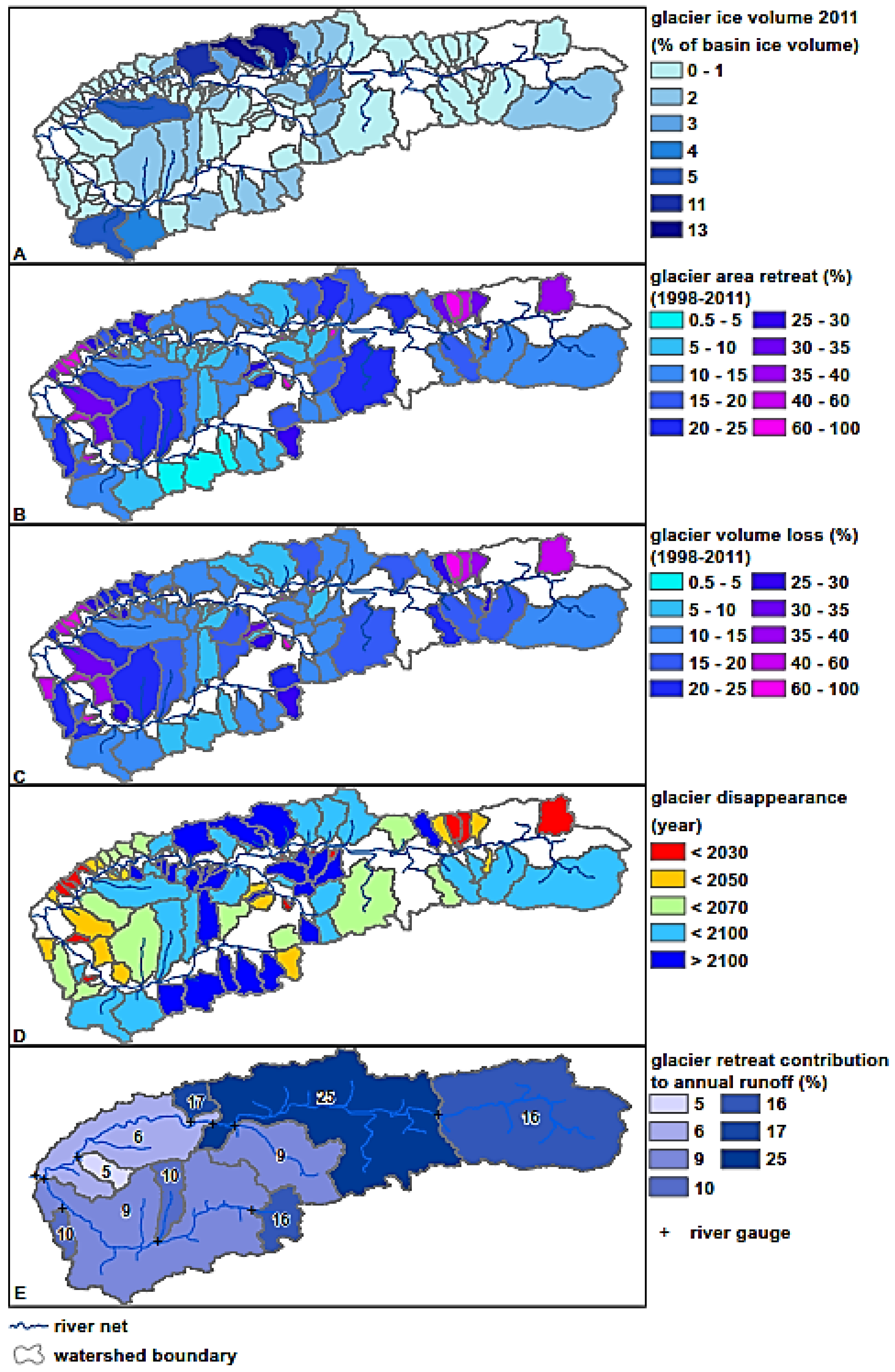
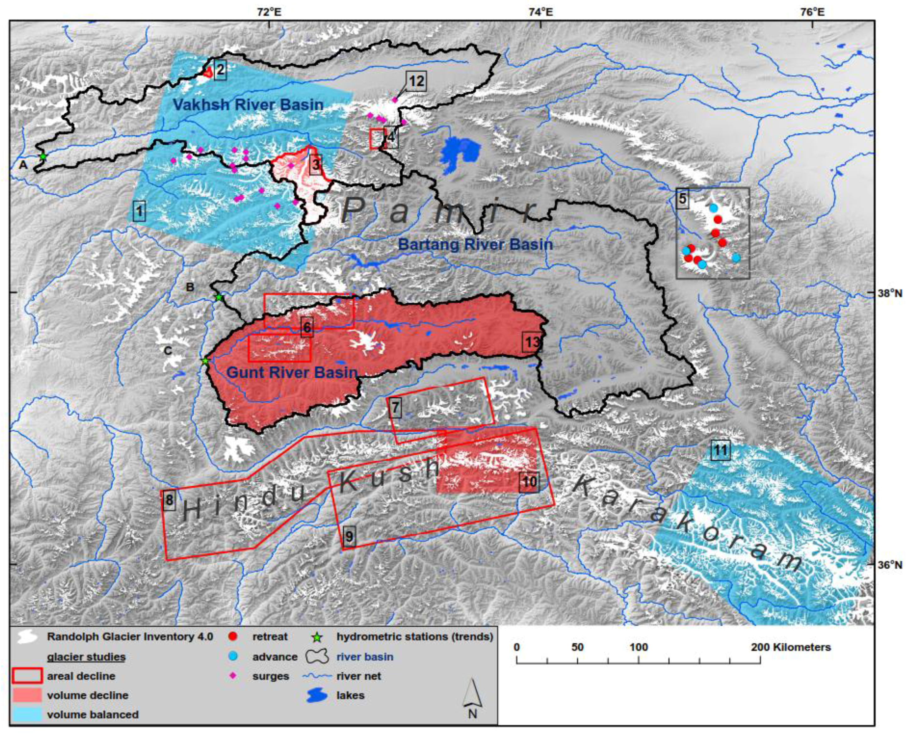
The results of glacier changes in the Gunt River Basin (Figure 2) show that the southern Pamirs are not part of the “Pamir-Karakoram Anomaly”, as originally assumed by Gardelle et al. [13]. A retreat of glacier areas in the Gunt River Basin by 14% (96 km²) took place between 1998 and 2011 (Table 1). Glacier retreat rates doubled in comparison to the period 1969–2002 [17]. The “accelerated retreat” reported for parts of the Rushan and Shugnan Pamir (No. 6 in Figure 1; [17]) can be extended to the entire southern Pamirs (No. 13 in Figure 1). This region of recent and intense glacier retreat can be classified into a larger scale of glacier retreat documented in the literature, including the Hindu Kush (Nos. 8 and 9 in Figure 1; [6,19]) and the Wakhan Pamir (No. 7 in Figure 1; [18]). If at all, a “Pamir Anomaly” of glaciers gaining mass can therefore only be existent in parts of the Northern Pamirs (No. 1 in Figure 1; [13]) and in the Chinese Pamirs (No. 5 in Figure 1; [4,5,20]). The findings of mass gaining glaciers in the Northern Pamirs can only be true for the late 20th and the early 21st century because studies regarding longer time periods identified volume losses (No. 3 in Figure 1; [14]) or area retreat (No. 4 in Figure 1; [16]) there. Nevertheless, long-term mass losses of the Fedchenko glacier are one order of magnitude smaller than, e.g., at Abramov glacier (Table 1; [37]) or than recent losses in the Southern Pamirs (Table 1 and Table 3).

In total, glaciers lost 5.3 ± 0.8 km³ of ice volume between 1998 and 2011 (12%), based on the GlabTop approach. Average thinning rates of glaciers were 0.53 m·y⁻¹ (Table 3). These results are in line with the results of Kääb et al. [20], who estimated thinning rates between 0.3 and 0.8 m·y⁻¹ for the Southern Pamirs (mean 0.55 m·y⁻¹; Table 3), using ICESat laser altimetry data. 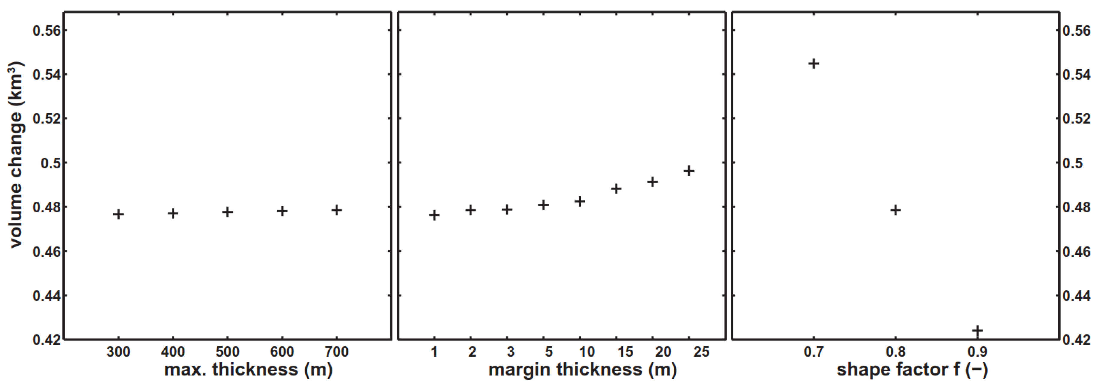Glacier wastage estimated with GRACE and a mass balance model ([26]; expressed as m of water column) is 15% larger (Table 3), but still within the range of the parameter uncertainty of the GlabTop results (Appendix A.1).

Ice thickness distribution models, therefore, appear to be an efficient option to estimate glacier volume change on the catchment scale. They are process based [58] and are independent from uncertain precipitation records. Their spatial resolution is higher than that of large-scale satellite approaches, and the combination of both seems beneficial. Exemplary, we validated such a model successfully on a large scale (entire river basin) by reviewing corresponding satellite-based approaches. The spatial resolution allows exploiting the model results on the subbasin scale, subsequently (Figure 2).

Glacier retreat in the Gunt River Basin takes place in all sub-basins without exception, but the magnitude of glacier area and volume retreat in the Gunt Basin is spatially heterogeneous (Figure 2B,C). The largest glacier wastage takes place at small glaciers in the western part of the catchment and at south-facing subbasins in the north-east parts of the catchment (Northern Alichur Range). The smallest glacier retreat takes place in the north-facing subbasins surrounding the highest mountains (Peak Karl Marx, Peak Engels). Subbasins storing the largest ice volumes (Figure 2A) show retreat rates of five to 15% (area and volume; Figure 2B,C) between 1998 and 2011.

Here, we assume linearly continuing retreat rates as a conservative (minimal) scenario of glacier retreat, based on the projections of Lutz et al. [65] and Pohl et al. [26]. In the subbasins of the western and north-eastern Gunt catchment, glacier coverage is expected to completely disappear already until 2030 (Figure 2D). Most other subbasins might be deglaciated until the year 2100 with potentially large impacts on the local fresh-water supply and traditional irrigation agriculture in the late ablation period (August, September). Nevertheless, subbasins storing the largest amounts of total basin-wide ice volumes, in the north-central and south-west catchment (Figure 2A), might still be glaciated for centuries, even if glacier retreat does not slow down due to potentially smaller retreat rates in higher elevations. This means that runoff rates of the Gunt River can still benefit from glacier melt for decades or even centuries, which is important for hydropower production and drinking water availability. However, local communities receive their fresh-water directly from tributaries, where irrigation ditches transport meltwater to gardens and settlements at the hillslopes. This water supply is endangered by the absence of glacier meltwater during the ablation period, which is the main growing season. In August and September, the basin hardly receives any rainfall, and snow cover has already disappeared (Pohl et al. [32,43]).

The contribution of glacier retreat to river runoff is relatively smaller in western subbasins (Figure 2E). Subbasins with smaller precipitation rates receive up to 25% of annual runoff from glacier retreat (Figure 2E). This means complete disappearance of glaciers will severely affect total river runoff in the more arid parts of the Pamirs (towards the east), which nowadays receive proportionally more meltwater from retreating glaciers. Regions of higher precipitation rates are less affected, and strengthening westerly precipitation [45,46] might potentially compensate for decreasing glacier meltwater. However, deglaciation most likely will leave a gap in river runoff amounts during summer months, because in the Western Pamirs, precipitation almost exclusively falls in winter and spring (see below).

On average, glacier retreat contributes 10% to the annual Gunt River runoff between 1998 and 2011, estimated based on two independent methods (Table 3). This robust estimation has recently been assimilated into a glacio-hydrological model by Tarasova et al. [33], who modeled melt rates of snow-free glacier ice to amount to 10% ± 4% of annual runoff.

Applying the mass balance results from Pohl et al. [26] (Table 3) to the classified glacier area of 707 km² [23] fractionizes their results into 13% runoff contribution from glacier retreat and 6% runoff contribution from perennial snow cover (Table 3). The glacier retreat contribution to annual runoff is in line with the results of the other two studies. Nevertheless, they modeled total glacier melt to contribute 30% of annual runoff (in the same basin) [26,32], but with a different hydrological model, which defines glacier melt as the meltwater of glacier ice plus snowmelt from glacier surfaces. The substantial difference to Tarasova et al. [33] can further be explained by the treatment of permanent snow and ice cover as “glaciers”, based on the application of gridded land cover data (MODIS MCD12Q1 dataset).

Runoff contribution from perennial snow cover seems to be rather large, especially under consideration that “glaciers” in the hydrological model are treated as infinite reservoirs (which is typical for conceptual models). The definition of “glacier retreat contribution to runoff” (also used in Figure 2E) quantifies the gap that will occur in river runoff, when glaciers will have completely disappeared. Snowmelt from glacier surfaces will still be present after glacier disappearance, but probably with a shift in runoff timing. The example shows that divergent definitions of which runoff fractions are incorporated into the term “glacier melt” can lead to larger uncertainties than those arising from glacio-hydrological modeling itself. A clear definition of runoff fractions is essential, when model results are to be used in water supply planning for communities that will be impacted by hydrologic change.

4.2. Runoff and Climate Trends versus Glacier Evolution

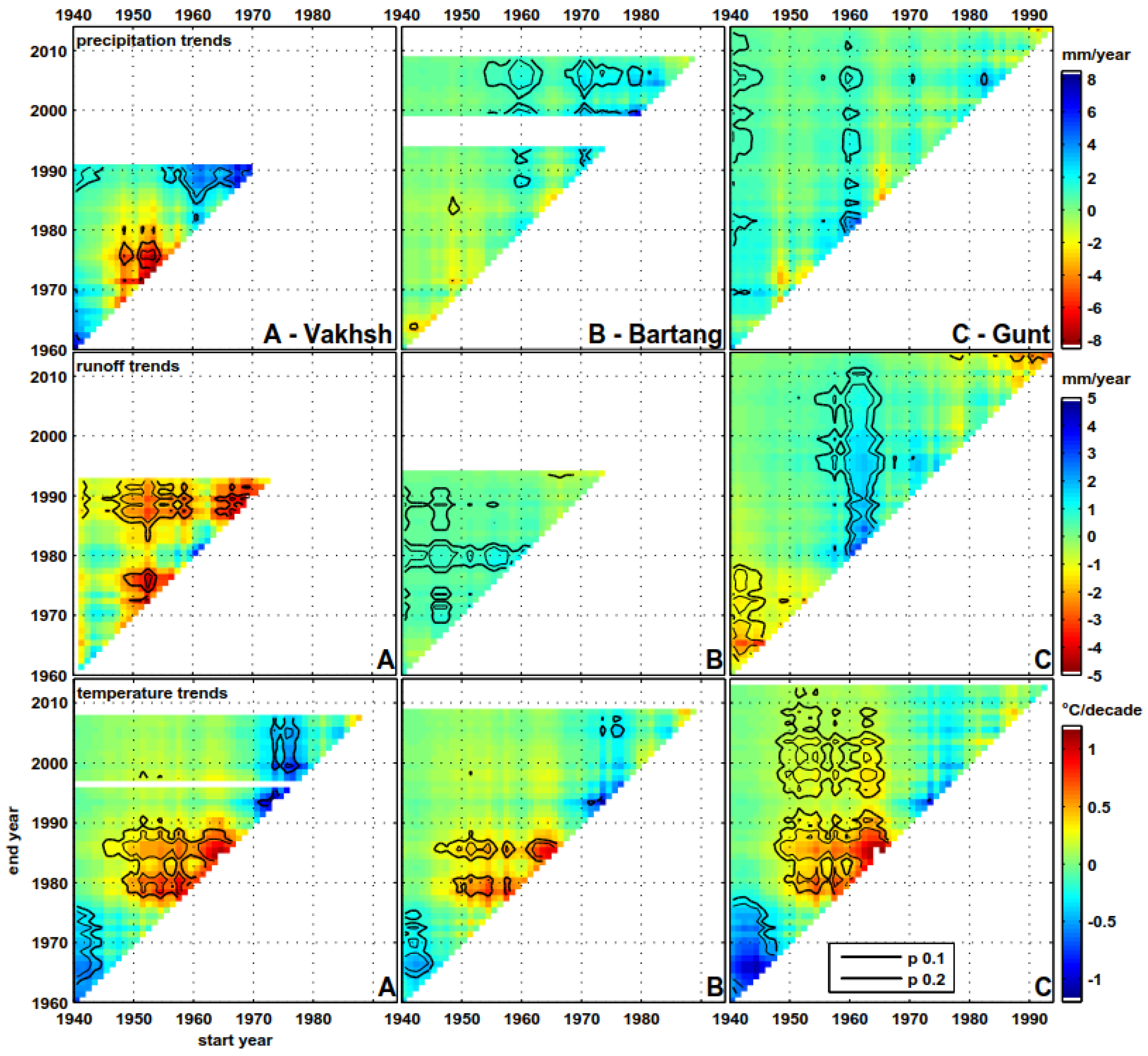
Trends in river runoff for the three river basins for different time periods are shown in Figure 3. River runoff in the Vakhsh Basin (North Pamirs) declines over large periods between 1940 and 1990 (Figure 3A, center row) with a magnitude of up to five millimeters per year. In contrast, river runoff in the Gunt Basin (South Pamirs) increases between 1955 and 2010 by up to 5 mm·y⁻¹ (Figure 3C, center row). Both trends are statistically significant at the 10% level. The Bartang River in the Central Pamirs shows stable runoff trends over decades (Figure 3B, center row).

Figure 3 allows a direct comparison of runoff trends (center row) with precipitation trends (top row) and temperature trends (bottom row). The River Gunt (Figure 3C) shows a statistically significant runoff decline between 1940 and the end of the 1970s, where the temperature trend shows intense cooling. Starting 1960, temperatures show a strong warming trend. Along with an increase in precipitation, runoff trends become positive for decades until recent times.

In the Vakhsh Basin (Figure 3A), river runoff declined in a statistically significant manner between 1950 and ca. 1980, although temperature shows a strong warming in that time, which is assumed to increase the meltwater contribution of glaciers. In the same time, precipitation trends show a strong decline of up to 8 mm·y⁻¹. This strong precipitation decline, which is obviously not observed in the South and Central Pamirs, probably caused the first period of negative runoff trends in the Vakhsh River basin, although the temperature was rising. A second period of runoff decline followed one decade later and lasted at least until 1994 (where the time series ends). Parallel to this runoff decline, precipitation rates increased significantly. This is surprising and might be explained by a statistically significant cooling of partly up to 1 °C per decade in July and August, between 1970 and 2010 (Figure 3A, bottom row). We suppose that increasing precipitation along with cooling temperatures caused higher glacier accumulation rates in the Vakhsh Basin in the late 20th and the beginning of the 21st century. This might explain the findings of balanced glacier mass budgets in the North-West Pamirs [13].

Similar characteristics were found in parts of the Upper Indus Basin: Fowler and Archer [64] explain the decline in river runoff in the Hunza Basin (Karakoram) by a decline of mean summer temperatures by 1 °C since 1961, causing glacier mass gain. Here, also a significant precipitation increase was detected [66]. Kapnick et al. [37] deduced a “prevailing hypothesis” from the literature for the Karakoram: increasing glacier accumulation occurs due to decreasing warm-season temperatures along with increasing precipitation rates.

We find a decline in summer temperatures (July, August) in all depicted climate stations used for the trend statistics after 1970 (Figure 3 bottom row). In the Northern Pamirs, this trend is persistent and statistically significant. In the Southern Pamirs (Figure 3C), the trend is statistically not significant, less pronounced and not persistent. Much more, a warming trend of ca. 0.2 °C per decade is statistically significant from 1950–2010. Assuming that the applied climate data are also representative for glaciated elevations, this could partly explain the largely divergent pattern of glacier evolution between the North and South Pamirs (Figure 1; Table 1).

On the other hand, the temporal patterns of temperature trends look quite similar in the North, Central and South Pamirs (Figure 3, bottom row) and seem to be similar to trends in the Karakoram and Hindu Kush [64]. Diverging patterns of glacier evolution might be driven by other (stronger) forces. When the cooling trend after 1970 is responsible for glacial mass gain in the Northern Pamirs and Karakoram, why not in the Southern Pamirs and Hindu Kush? The elevation effect and precipitation characteristics seem to be stronger proxies for diverging patterns of glacial evolution.

The impact of glacier evolution on river discharge in the Pamirs follows a distinct spatial pattern: the Gunt River recently receives 10% ± 4% of the annual river discharge from glacier retreat [33], while the runoff trend is significantly rising since the end of the 1950s. This is comparable to those tributaries of the Upper Indus, which drain the Hindu Kush. There, glacier retreat causes rising river flows [67,68]. In contrast, the Vakhsh River basin shows decreasing runoff trends along with glacier mass gain or moderate glacier mass losses. This is comparable to the Hunza Catchment draining the Northern Karakoram [68].

Therefore, runoff trends in the Pamir-Hindu Kush-Karakoram region show the same spatial pattern as glacier evolution does (Figure 1), an anomaly in the North-West Pamirs and North Karakoram versus a distinct glacier and hydrological change in the South Pamirs and Hindu Kush. Meanwhile, the Bartang River (Central Pamirs) shows almost no significant runoff trend over several decades (Figure 3C, center row), which outlines a stable runoff regime, potentially because the two runoff extremes cancel each other out between North and South Pamir.

4.3. Precipitation Pattern versus Glacier Evolution

We believe that the cooling of summer temperatures since the 1970s plays a crucial role in glacier mass gain in the Northern Pamirs and Karakoram. However, the cooling trend cannot explain why glaciers in the Southern Pamirs and Hindu Kush are retreating rapidly. Therefore, precipitation characteristics require a more detailed investigation.

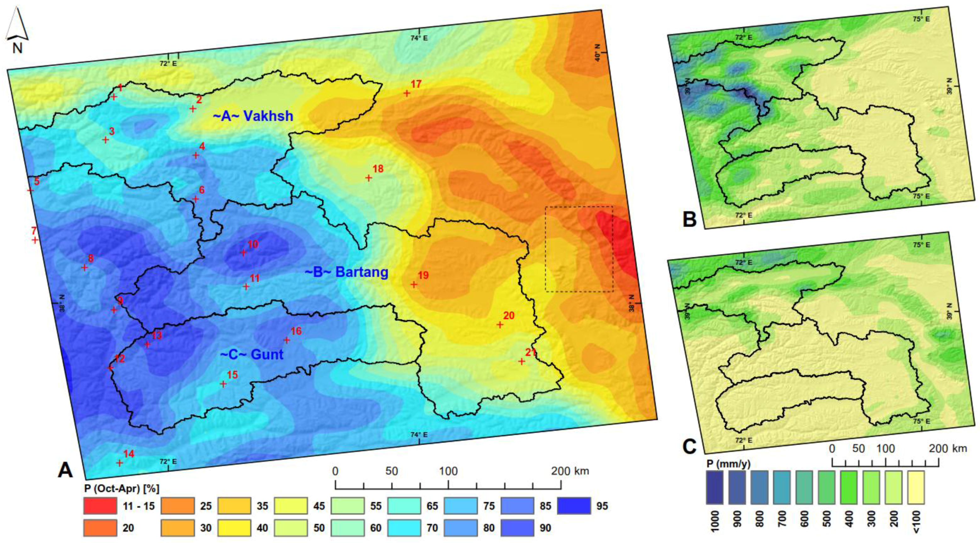
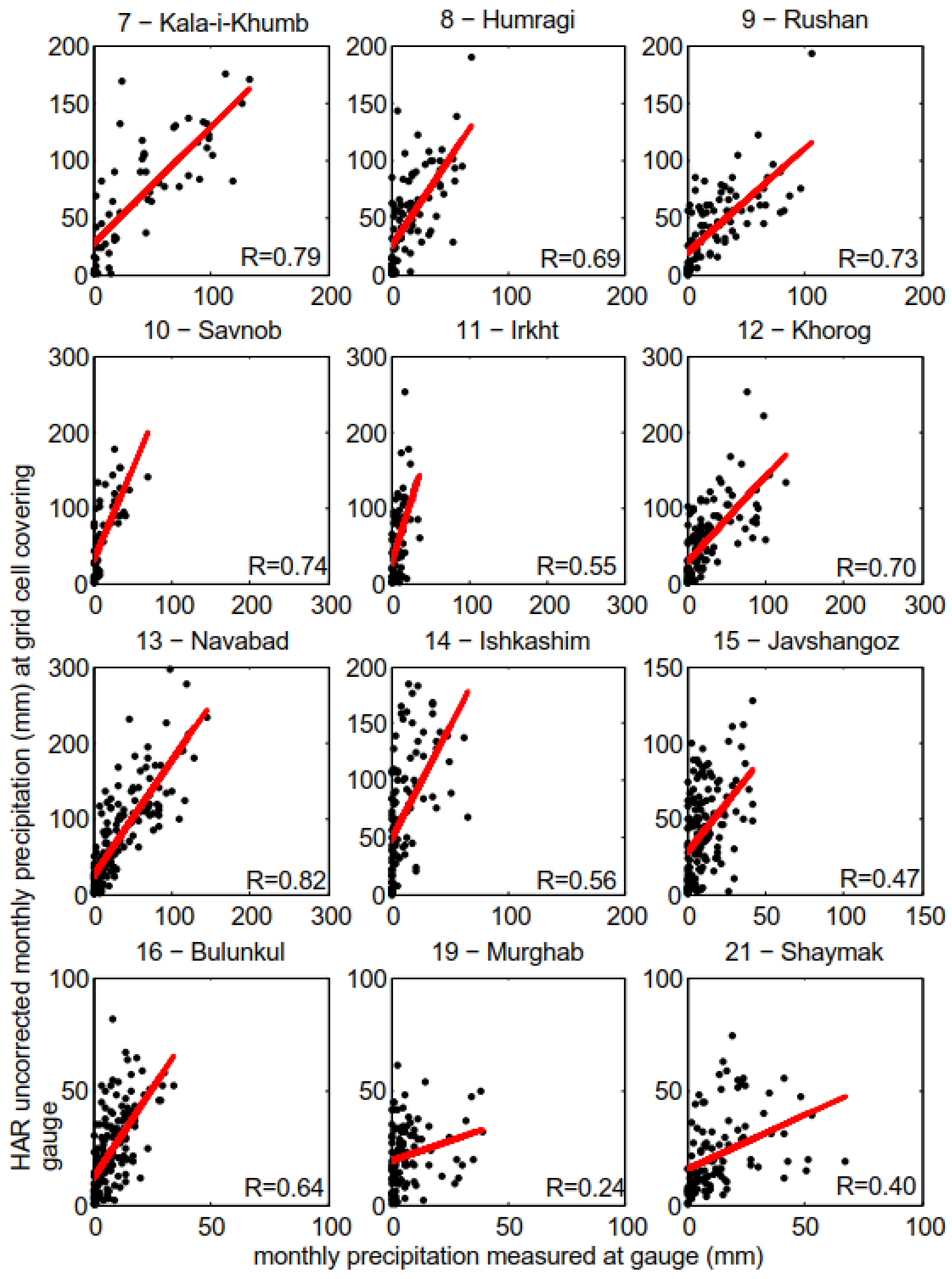
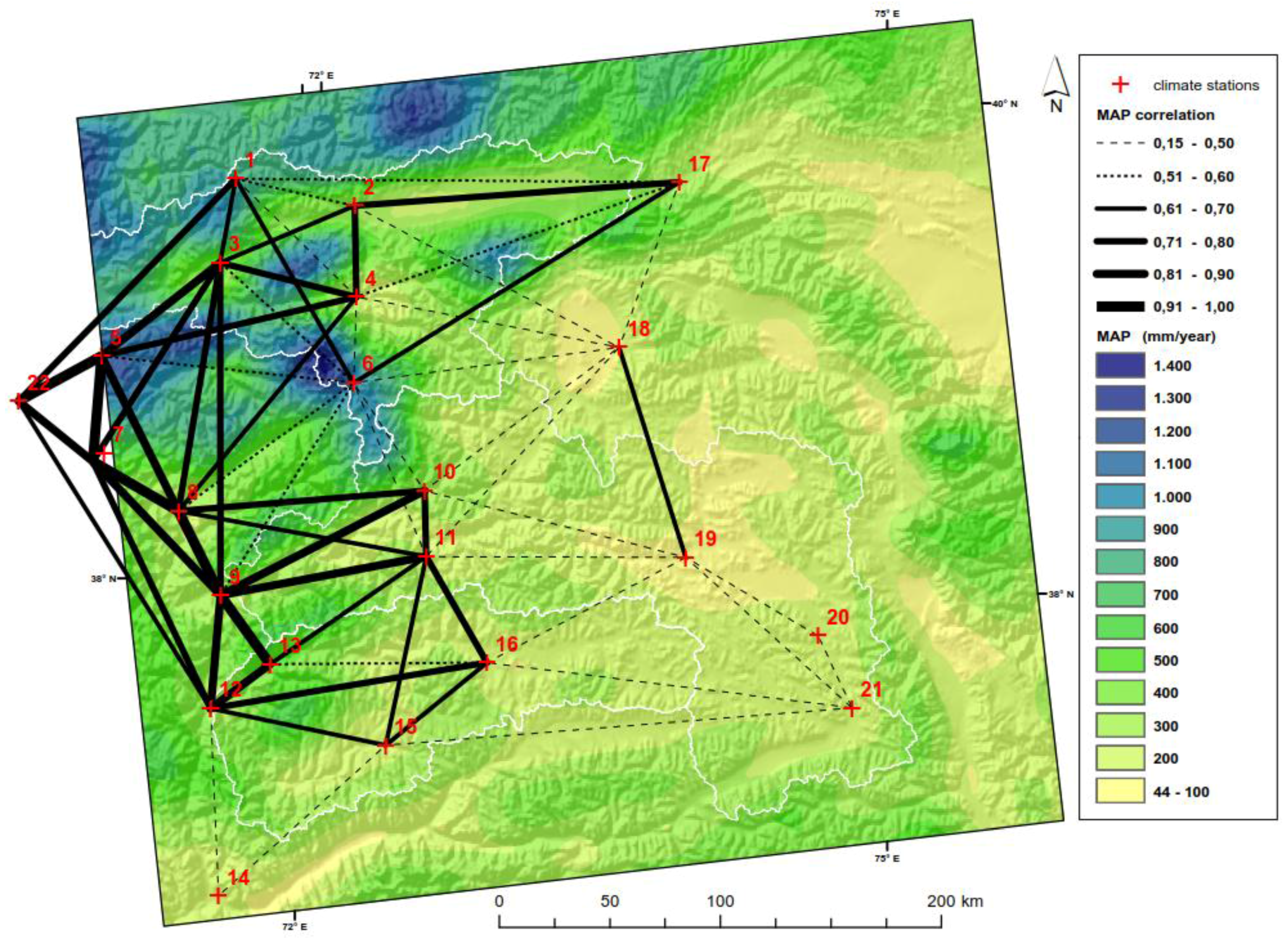
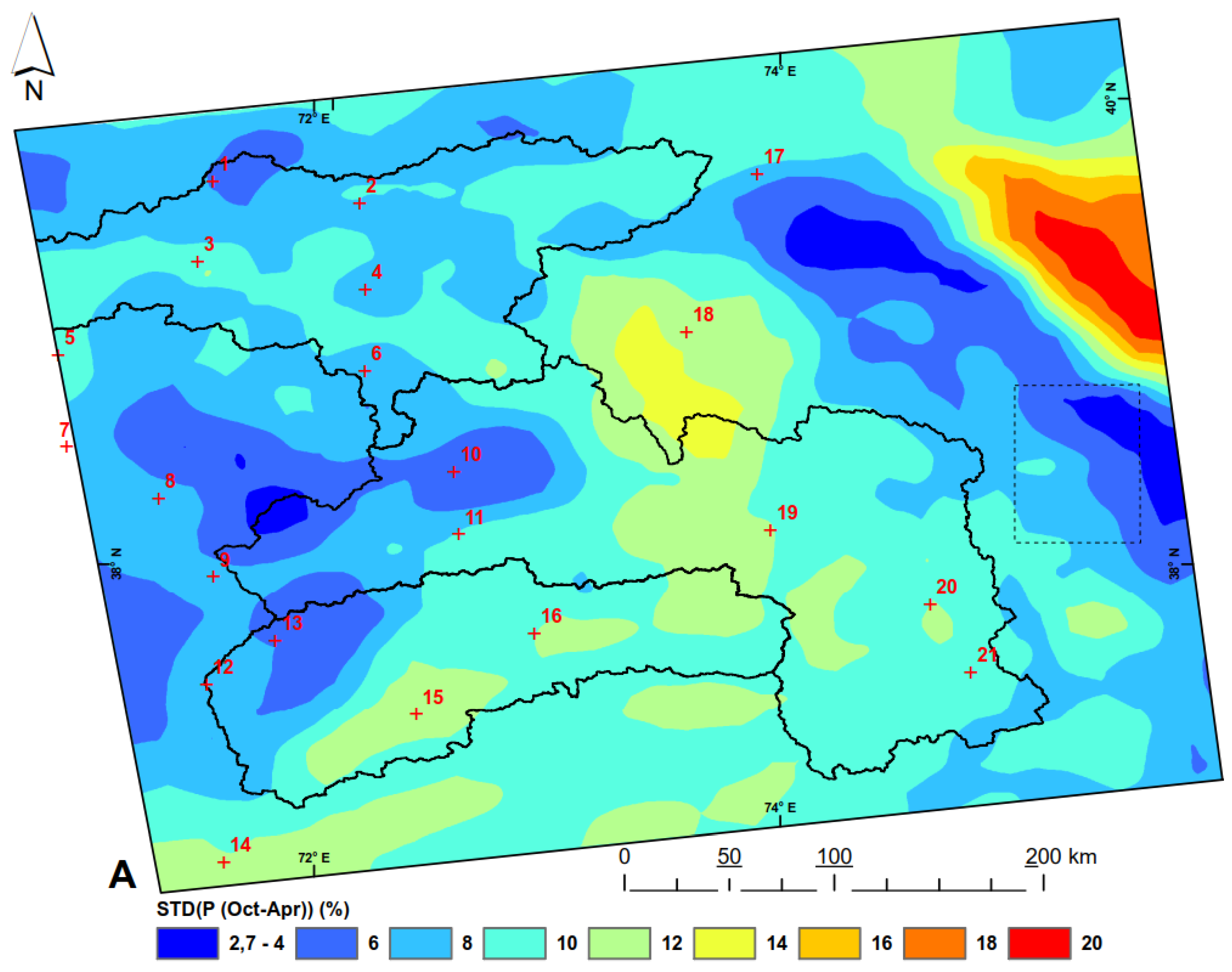
Generally, assumptions on precipitation characteristics have to be seen in the light of the uncertainties depicted in the Methods section. We figured out that high-resolution data of the High Asia Refined analysis (HAR; [39]) provides reliable information on winter precipitation rates (Figure 4A), stemming from westerly wind systems. In the opposite way, convective summer precipitation in the Eastern Pamirs is less well reflected by the HAR dataset. Absolute magnitudes of precipitation had to be bias-adjusted (Figure A2).

Bias-corrected HAR precipitation data from 2001 to 2011 imply that the contrasting glacier evolution in the North and South Pamirs can potentially be explained by the distribution of basin-wide precipitation. In the Vakhsh Basin, 24% of basin-wide precipitation falls directly on glaciated areas which cover 17% of the basin area (Figure 5A). In the Gunt Basin, it is only 6% of annual basin-wide precipitation that directly falls on glaciers covering only 5% of the basin area (Figure 5C; Table 2). We assume that the “unique water cycle” of the Karakoram [37] is also present in the nival regime of the Western, Central and Southern Pamirs, where up to 95% of precipitation falls in winter (Figure 4). This means that in the North Pamirs, at least 24% of annual precipitation (Figure 5A) contributes to glacier accumulation. In contrast, up to 94% of annual precipitation in the South Pamirs is preset to melt within the seasonal water cycle (Figure 5C). Further, the ratio of precipitation on glaciers to glacier area shows that glacier areas in the Vakhsh basin receive proportionally more precipitation than glacier areas in the South Pamirs (Figure 5).

Higher accumulation rates in the north can partly explain why runoff trends tend to be negative there and vice versa. Rising runoff trends in the South Pamirs are likely to be caused by increasing westerly precipitation (Figure 3C, top row) in addition to warming-induced glacier retreat (Figure 3C, bottom row). Thus, an increase in westerly precipitation [45,46] in both regions causes glacier mass gain in the Northern Pamirs and rising river flows in the Southern Pamirs.

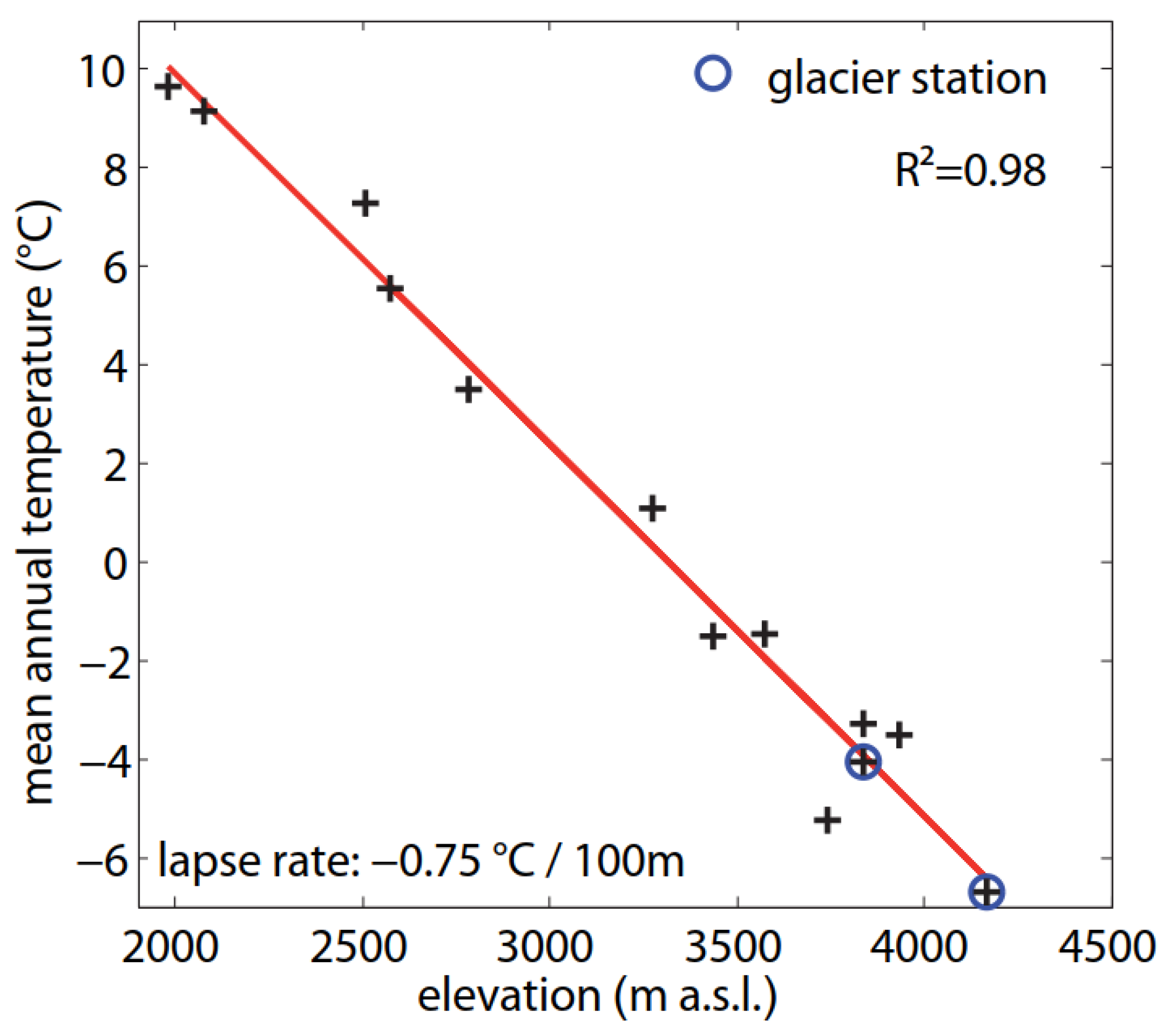
Altitudinal precipitation distribution (Figure 5) further shows that in the Vakhsh Basin, 46% of annual precipitation falls below the permafrost boundary (ca. 3800 m a.s.l.; [17]). At altitudes below permafrost, meltwater can better infiltrate into soils, where it is prone to evaporation and transpiration by plants (“green water” [69]). In the Gunt River Basin, 86% of annual precipitation falls on potential permafrost sites, which allow less infiltration into the ground and cause higher fractions of surface runoff.

A plausible scenario is that precipitation increase (Figure 3, top row; [45,46]) causes higher rates of green water losses and glacier accumulation rates in the Vakhsh Basin, and therefore, runoff declines (Figure 3A, center row). In contrast, increasing precipitation in the Gunt Basin is followed by a more or less direct increase in river runoff (Figure 3C, center row) due to limited glacier accumulation and limited meltwater infiltration (Figure 5C). The winter precipitation regime itself, as proposed by Kapnick et al. [37] for the Karakoram, cannot explain diverging trends of glacial evolution in the Pamirs, because also shrinking glaciers in the Southern Pamirs receive almost exclusively winter precipitation (Figure 4A).

The “elevation effect” [12,36] seems to advantage some glaciated regions in the Pamirs, because the smallest rates of glacier retreat occur around the highest peaks: locally around Peak Karl Marx (6723 m) in the South Pamirs (Figure 2B), more regionally in the Fedchenko area (up to 7495 m) in the North Pamirs and in the Muztaq Ata region (>7500 m) in the East Pamirs. Associated glacier systems might benefit from those “water towers” and yearlong temperatures below the freezing point. Nevertheless, Figure 4 illustrates that highest precipitation rates of up to 1400 mm·y⁻¹ are much more a regional feature than an altitudinal effect (Figure 5). Thus, glaciers in the Northern Pamirs are supposed to simply benefit from their position towards the westerly wind systems and declining temperatures (see Section 4.2). In this context, the hypothesis of Cannon et al. [46], saying the Karakoram Ranges might be more prone to orographic blocking due to intensification and a northward shift of westerly wind systems, might also be meaningful for the high Pamirs.

Further influences on the relationship between glaciers and runoff, such as debris cover and (scale-dependent) aspect-distributions of glaciers, have not been investigated in this study, e.g., debris cover may have an additional impact on glaciers’ response to climate change [70].

5. Conclusions

The hypothetical “Pamir-Karakoram-Anomaly” [13] cannot be extended to the Southern Pamirs. Much more, the extent of glacier retreat in the Southern Pamirs is similar to that in the Hindu Kush. Furthermore, runoff trends in the Southern Pamirs are similar to those in the Hindu Kush, where glacier retreat causes rising river flows (Figure 2E; Table 3; [67,68]). In contrast, glacier evolution and runoff trends in the Northern Pamirs are similar to those in the Northern Karakoram. In both regions, balanced or gaining glacier mass budgets coincide with a decline in river runoff. Runoff trends seem to be a strong proxy for glacier evolution in the Pamir-Hindu Kush-Karakoram region, but are not frequently used when glacial change is investigated.

The winter precipitation regime in the Pamirs and Hindu Kush provides only a weak explanation for glaciers gaining mass. Those parts of the Pamirs that receive more than 90% winter precipitation show accelerated rates of glacier retreat. Meanwhile, more balanced glaciers in the Fedchenko region receive 15%–30% of annual precipitation in summer (May–September). Furthermore, the East Hindu Kush receives mostly winter precipitation [39], but area-wide glacier wastage takes place there, as well.

The smallest rates of glacier retreat in the Pamirs are found close to mountains higher than 6700 m a.s.l. This underlines the idea of Hewitt [12,36], who makes “the elevation effect” and accumulation characteristics, such as all-year accumulation of glaciers, responsible for mass gaining glaciers in the Karakoram. On the first view, this concept might be true in the Pamirs, as well. Regarding local climatic pattern and trends more closely, two meteorological forces might rather be responsible for balanced glacier mass budgets in the Northern Pamirs:

• A cooling of summer temperatures after 1970.
• Highest precipitation rates up to 1400 mm·y⁻¹ (Figure 4B,C; Figure A5) in comparison to adjacent regions and a large fraction of annual basin-wide precipitation falling directly on glaciers.

Both forces are much more pronounced in the Northern Pamirs than in the south, and they are congruent to the Northern Karakoram. There, Fowler and Archer [64] detected a decline in summer temperatures since 1961. Immerzeel et al. [71] discovered mean annual precipitation amounts between 700 and beyond 1000 mm·y⁻¹ at elevations above 5000 m in the Hunza Basin. The winter precipitation regime [37] might further strengthen glacier mass gain, but the actual drivers seem to be absolute precipitation amounts along with declining summer temperatures. It can only be hypothesized that precipitation increase contributes to stable glacier mass balances in the Northern Pamirs, because the time series end in 1994. Further, increasing winter precipitation rates alone cannot explain glacier mass gain, because in the Southern Pamirs, glaciers are retreating, although a stable positive precipitation trend is present since 1960.

There, the Gunt River receives approximately 10% of annual runoff from glacier retreat, and river discharge will still be enhanced by glacier wastage for decades or even centuries. Nevertheless, locally, settlements will be affected by water scarcity during the vegetation period within the next few decades, when entire subbasins will be deglaciated. The following hypotheses on the socio-economic consequences of glacier wastage in the Pamirs are deduced here:

• Glacier wastage will rapidly impact mountain communities, which allocate glacier meltwater during the ablation and vegetation period directly to irrigation ditches to their fields.
• In contrast, riverine settlements located downstream at larger rivers will be less affected by glacier wastage in the next few decades, including negligible effects on hydropower and irrigation agriculture. Much more, glacier retreat enhances river discharge and fresh water availability of the main receiving streams.
• Migration from mountain areas into riverine settlements might be enhanced. Urbanization might be the first consequence of glacier wastage, rather than absolute water shortage, but highly dependent on the scale we regard when investigating hydrological change in the (Southern) Pamirs and adjacent regions.

Accelerated glacier wastage in the Southern Pamirs is probably enhanced by an accumulation regime, which receives generally less precipitation, in absolute amounts, as well as the percentage of annual basin-wide precipitation falling directly on glaciers. Therefore, we assume that Northern Pamir glaciers are “protected” by generally higher accumulation rates and an “all-year accumulation regime” [36] due to higher elevations, which coincide with lower temperatures. In this environment, the detected cooling of summer temperatures caused glaciers to gain mass and river runoff to decline. Parallels to the Karakoram are obvious.

The regional patterns of contradicting glaciological and hydrological trends in the Pamirs, Hindu Kush and Karakoram are indeed similar and were detected by integrating patchy glaciological knowledge into the concept of comparative hydrology. We conclude that comparative hydrology yields large potential to study glacier evolution where glacier observations are spatially incomplete and temporally restricted to the last few decades due to limited availability of satellite data. For glacier evolution studies of entire mountain ranges, we suggest to incorporate runoff trend information more systematically and frequently. River discharge time series incorporate the catchment integral of glacier fluxes in space and time, while satellite glaciology provides spatially explicit, but also restricted information as points on the time axis. Both brought together can help to better understand climatic change and its actual impact on water resources and communities. Especially in Central Asia, in the states of the former Soviet Union, numerous runoff time series of glaciated basins are available since the 1940s.

We want to highlight the importance of in situ measurements in this water-scarce region. After 1993, investments in equipment and staff have collapsed, so that many data series have not been updated or their quality suffered. Compared to other climate-sensitive mountain regions, the length of the data series is outstanding. Prolongation of the hydro-climatic time series is a great opportunity for climate change research and also essential for the evaluation of global gridded datasets. Therefore, financial support and scientific cooperation are needed to carry forward the hydro-meteorological measurements in the 21st century.

References

1. Varis, O. Resources: Curb vast water use in Central Asia. Nature 2014, 514, 27–29. [Google Scholar] [CrossRef] [PubMed]
2. BTI. Tajikistan Country Report; Bertelsmann Stiftung: Gütersloh, Germany, 2012; Available online: http://www.bti-project.de/uploads/tx_itao_download/BTI_2012_Tajikistan.pdf (accessed on 6 June 2017).
3. Aizen, V.B. Pamir glaciers. In Encyclopedia of Snow, Ice and Glaciers; Singh, V.P., Singh, P., Haritashya, U.K., Eds.; Springer: Dordrecht, The Netherlands, 2011; pp. 813–815. [Google Scholar]
4. Yao, T.; Thompson, L.; Yang, W.; Yu, W.; Gao, Y.; Guo, X.; Yang, X.; Duan, K.; Zhao, H.; Xu, B.; et al. Different glacier status with atmospheric circulations in Tibetan Plateau and surroundings. Nat. Clim. Chang. 2012, 2, 663–667. [Google Scholar] [CrossRef]
5. Bolch, T.; Kulkarni, A.; Kääb, A.; Huggel, C.; Paul, F.; Cogley, J.G.; Frey, H.; Kargel, J.S.; Fujita, K.; Scheel, M.; et al. The state and fate of Himalayan glaciers. Science 2012, 336, 310–314. [Google Scholar] [CrossRef] [PubMed]
6. Sarikaya, M.A.; Bishop, M.P.; Shroder, J.F.; Olsenholler, J.A. Space-based observations of Eastern Hindu Kush glaciers between 1976 and 2007, Afghanistan and Pakistan. Remote Sens. Lett. 2012, 3, 77–84. [Google Scholar] [CrossRef]
7. Farinotti, D.; Longuevergne, L.; Moholdt, G.; Duethmann, D.; Mölg, T.; Bolch, T.; Vorogushyn, S.; Güntner, A.; Molg, T.; Bolch, T.; et al. Substantial glacier mass loss in the Tien Shan over the past 50 years. Nat. Geosci. 2015, 8, 716–722. [Google Scholar] [CrossRef]
8. Liu, Q.; Liu, S. Response of glacier mass balance to climate change in the Tianshan Mountains during the second half of the twentieth century. Clim. Dyn. 2016, 46, 303–316. [Google Scholar] [CrossRef]
9. Zhang, Y.; Enomoto, H.; Ohata, T.; Kitabata, H.; Kadota, T.; Hirabayashi, Y. Projections of glacier change in the Altai Mountains under twenty-first century climate scenarios. Clim. Dyn. 2016. [Google Scholar] [CrossRef]
10. Gardelle, J.; Berthier, E.; Arnaud, Y. Slight mass gain of Karakoram glaciers in the early twenty-first century. Nat. Geosci. 2012, 5, 322–325. [Google Scholar] [CrossRef]
11. Kääb, A.; Berthier, E.; Nuth, C.; Gardelle, J.; Arnaud, Y. Contrasting patterns of early twenty-first-century glacier mass change in the Himalayas. Nature 2012, 488, 495–498. [Google Scholar] [CrossRef] [PubMed]
12. Hewitt, K. The Karakoram anomaly? Glacier expansion and the “elevation effect”, Karakoram Himalaya. Mt. Res. Dev. 2005, 25, 332–340. [Google Scholar] [CrossRef]
13. Gardelle, J.; Berthier, E.; Arnaud, Y.; Kääb, A. Region-wide glacier mass balances over the Pamir-Karakoram-Himalaya during 1999–2011. Cryosphere 2013, 7, 1263–1286. [Google Scholar] [CrossRef]
14. Lambrecht, A.; Mayer, C.; Aizen, V.; Floricioiu, D.; Surazakov, A. The evolution of Fedchenko glacier in the Pamir, Tajikistan, during the past eight decades. J. Glaciol. 2014, 60, 233–244. [Google Scholar] [CrossRef]
15. Holzer, N.; Vijay, S.; Yao, T.; Xu, B.; Buchroithner, M.; Bolch, T. Four decades of glacier variations at Muztagh Ata (eastern Pamir): A multi-sensor study including Hexagon KH-9 and Pléiades data. Cryosphere 2015, 9, 2071–2088. [Google Scholar] [CrossRef]
16. Khromova, T.E.; Osipova, G.B.; Tsvetkov, D.G.; Dyurgerov, M.B.; Barry, R.G. Changes in glacier extent in the eastern Pamir, Central Asia, determined from historical data and ASTER imagery. Remote Sens. Environ. 2006, 102, 24–32. [Google Scholar] [CrossRef]
17. Mergili, M.; Kopf, C.; Müllebner, B.; Schneider, J.F. Changes of the cryosphere and related geohazards in the high-mountain areas of Tajikistan and Austria: A comparison. Geogr. Ann. 2012. [Google Scholar] [CrossRef]
18. Haritashya, U.K.; Bishop, M.P.; Shroder, J.F.; Bush, A.B.G.; Bulley, H.N.N. Space-based assessment of glacier fluctuations in the Wakhan Pamir, Afghanistan. Clim. Chang. 2009, 94, 5–18. [Google Scholar] [CrossRef]
19. Sarikaya, M.A.; Bishop, M.P.; Shroder, J.F.; Ali, G. Remote-sensing assessment of glacier fluctuations in the Hindu Raj, Pakistan. Int. J. Remote Sens. 2013, 34, 3968–3985. [Google Scholar] [CrossRef]
20. Kääb, A.; Treichler, D.; Nuth, C.; Berthier, E. Brief communication: Contending estimates of 2003–2008 glacier mass balance over the Pamir–Karakoram–Himalaya. Cryosphere 2015, 9, 557–564. [Google Scholar] [CrossRef]
21. Barandun, M.; Huss, M.; Sold, L.; Farinotti, D.; Azisov, E.; Salzmann, N.; Usubaliev, R.; Merkushkin, A.; Hoelzle, M. Re-analysis of seasonal mass balance at Abramov glacier 1968–2014. J. Glaciol. 2015, 61, 1103–1117. [Google Scholar] [CrossRef]
22. Kotlyakov, V.M.; Osipova, G.B.; Tsvetkov, D.G. Monitoring surging glaciers of the Pamirs, Central Asia, from space. Ann. Glaciol. 2008, 48, 125–134. [Google Scholar] [CrossRef]
23. Lindner, M. Rezente Gletscheränderung im Einzugsgebiet des Gunts (Tadschikistan). Master‘s Thesis, Institut für Geographie, Leopold-Franzens-Universität Innsbruck, Innsbruck, Austria, 2013. (In German). [Google Scholar]
24. Gardner, A.S.; Moholdt, G.; Cogley, J.G.; Wouters, B.; Arendt, A.A.; Wahr, J.; Berthier, E.; Hock, R.; Pfeffer, W.T.; Kaser, G.; et al. A reconciled estimate of glacier contributions to sea level rise: 2003 to 2009. Science 2013, 340, 852–857. [Google Scholar] [CrossRef] [PubMed]
25. Jacob, T.; Wahr, J.; Pfeffer, W.T.; Swenson, S. Recent contributions of glaciers and ice caps to sea level rise. Nature 2012, 482, 514–518. [Google Scholar] [CrossRef] [PubMed]
26. Pohl, E.; Gloaguen, R.; Andermann, C.; Knoche, M. Glacier melt buffers river runoff in the Pamir Mountains. Water Resour. Res. 2017. [Google Scholar] [CrossRef]
27. Chevallier, P.; Pouyaud, B.; Mojaïsky, M.; Bolgov, M.; Olsson, O.; Bauer, M.; Froebrich, J. River flow regime and snow cover of the Pamir Alay (Central Asia) in a changing climate. Hydrol. Sci. J. 2014, 59, 1491–1506. [Google Scholar] [CrossRef]
28. Konovalov, V.G.; Shchetinnicov, S. Evolution of glaciation in the Pamiro-Alai mountains and its effect on river run-off. J. Glaciol. 1994, 40, 149–157. [Google Scholar] [CrossRef]
29. Unger-Shayesteh, K.; Vorogushyn, S.; Farinotti, D.; Gafurov, A.; Duethmann, D.; Mandychev, A.; Merz, B. What do we know about past changes in the water cycle of Central Asian headwaters? A review. Glob. Planet Chang. 2013. [Google Scholar] [CrossRef]
30. Hagg, W.; Hoelzle, M.; Wagner, S.; May, E.; Klose, Z. Glacier and runoff changes in the Rukhk catchment, upper Amu-Darya basin until 2050. Hydrol. Earth Syst. Sci. Discuss. 2011, 8, 1507–1540. [Google Scholar] [CrossRef]
31. Kure, S.; Jang, S.; Ohara, N.; Kavvas, M.L.; Chen, Z.Q. Hydrologic impact of regional climate change for the snowfed and glacierfed river basins in the Republic of Tajikistan: Hydrological response of flow to climate change. Hydrol. Process. 2013, 27, 4057–4070. [Google Scholar] [CrossRef]
32. Pohl, E.; Knoche, M.; Gloaguen, R.; Andermann, C.; Krause, P. Sensitivity analysis and implications for surface processes from a hydrological modelling approach in the Gunt catchment, high Pamir Mountains. Earth Surf. Dyn. 2015, 3, 333–362. [Google Scholar] [CrossRef]
33. Tarasova, L.; Knoche, M.; Dietrich, J.; Merz, R. Effects of input discretization, model complexity and calibration strategy on model performance in a data-scarce glacierized catchment in Central Asia. Water Resour. Res. 2016, 52, 4674–4699. [Google Scholar] [CrossRef]
34. Reggiani, P.; Rientjes, T.H.M. A reflection on the long-term water balance of the Upper Indus Basin. Hydrol. Res. 2014, 46, 446–462. [Google Scholar] [CrossRef]
35. Sivapalan, M. The secret to “doing better hydrological science”: Change the question! Hydrol. Process. 2009, 23, 1391–1396. [Google Scholar] [CrossRef]
36. Hewitt, K. Glacier Change, concentration, and elevation effects in the Karakoram Himalaya, Upper Indus Basin. Mt. Res. Dev. 2011, 31, 188–200. [Google Scholar] [CrossRef]
37. Kapnick, S.B.; Delworth, T.L.; Ashfaq, M.; Malyshev, S.; Milly, P.C.D. Snowfall less sensitive to warming in Karakoram than in Himalayas due to a unique seasonal cycle. Nat. Geosci. 2014, 7, 1–7. [Google Scholar] [CrossRef]
38. Kaser, G.; Grosshauser, M.; Marzeion, B. Contribution potential of glaciers to water availability in different climate regimes. Proc. Natl. Acad. Sci. USA 2010, 107, 20223–20227. [Google Scholar] [CrossRef] [PubMed]
39. Maussion, F.; Scherer, D.; Mölg, T.; Collier, E.; Curio, J.; Finkelnburg, R. Precipitation seasonality and variability over the Tibetan Plateau as resolved by the High Asia Reanalysis. J. Clim. 2014, 27, 1910–1927. [Google Scholar] [CrossRef]
40. Pfeffer, W.T.; Arendt, A.A.; Bliss, A.; Bolch, T.; Cogley, J.G.; Gardner, A.S.; Hagen, J.-O.; Hock, R.; Kaser, G.; Kienholz, C.; et al. The Randolph Glacier Inventory: A globally complete inventory of glaciers. J. Glaciol. 2014, 60, 537–552. [Google Scholar] [CrossRef]
41. Peel, M.C.; Finlayson, B.L.; McMahon, T.A. Updated world map of the Köppen-Geiger climate classification. Hydrol. Earth Syst. Sci. 2007, 11, 1633–1644. [Google Scholar] [CrossRef]
42. Aizen, V.B.; Mayewski, P.A.; Aizen, E.M.; Joswiak, D.R.; Surazakov, A.B.; Kaspari, S.; Grigholm, B.; Krachler, M.; Handley, M.; Finaev, A. Stable-isotope and trace element time series from Fedchenko glacier (Pamirs) snow/firn cores. J. Glaciol. 2009, 55, 275–291. [Google Scholar] [CrossRef]
43. Pohl, E.; Gloaguen, R.; Seiler, R. Remote sensing-based assessment of the variability of winter and summer precipitation in the Pamirs and their effects on hydrology and hazards using harmonic time series analysis. Remote Sens. 2015, 7, 9727–9752. [Google Scholar] [CrossRef]
44. Meier, C.; Knoche, M.; Merz, R.; Weise, S.M. Stable isotopes in river waters in the Tajik Pamirs: Regional and temporal characteristics. Isot. Environ. Health Stud. 2013, 49, 542–554. [Google Scholar] [CrossRef] [PubMed]
45. Machguth, H. Atmospheric science: Glaciers between two drivers. Nat. Clim. Chang. 2013, 4, 12–13. [Google Scholar] [CrossRef]
46. Cannon, F.; Carvalho, L.M.V.; Jones, C.; Bookhagen, B. Multi-annual variations in winter westerly disturbance activity affecting the Himalaya. Clim. Dyn. 2014. [Google Scholar] [CrossRef]
47. Jalilov, S.-M.; Varis, O.; Keskinen, M. Sharing Benefits in Transboundary Rivers: An experimental case study of Central Asian water-energy-agriculture nexus. Water 2015, 7, 4778–4805. [Google Scholar] [CrossRef]
48. World Bank. Final Reports Related to the Proposed Rogun HPP; World Bank: Washington, DC, USA, 2014; Available online: http://www.worldbank.org/en/country/tajikistan/brief/final-reports-related-to-the-proposed-rogun-hpp (accessed on 6 June 2017).
49. Hauser, M. The UNESCO Map of the Pamirs and its implications of ecotourism in Tajikistan. Avaliable online: http://www.mountaincartography.org/publications/papers/papers_nuria_04/hauser.pdf (accessed on 6 June 2017).
50. Jarvis, A.; Reuter, H.I.; Nelson, A.; Guevara, E. Hole-Filled Seamless SRTM Data V4; Technical Report; International Centre for Tropical Agriculture (CIAT): Palmira, Colombia, 2008. [Google Scholar]
51. Finger, D.; Vis, M.; Huss, M.; Seibert, J. The value of multiple dataset calibration versus model complexity for improving the performance of hydrological models in mountain catchments. Water Resour. Res. 2015, 51, 1939–1958. [Google Scholar] [CrossRef]
52. Mölg, T.; Maussion, F.; Scherer, D. Mid-latitude westerlies as a driver of glacier variability in monsoonal High Asia. Nat. Clim. Chang. 2013, 4, 68–73. [Google Scholar] [CrossRef]
53. Keeratikasikorn, C.; Trisirisatayawong, I. Reconstruction of 30 m DEM from 90 m DEM with bicubic polynomial interpolation method. Int. Arch. Photogramm. Remote Sens. Spat. Inf. Sci. 2008, 37 Pt B1, 90–93. [Google Scholar]
54. Paul, F.; Barry, R.G.; Cogley, J.G.; Frey, H.; Haeberli, W.; Ohmura, A.; Ommanney, C.S.L.; Raup, B.; Rivera, A.; Zemp, M. Recommendations for the compilation of glacier inventory data from digital sources. Ann. Glaciol. 2009, 50, 119–126. [Google Scholar] [CrossRef]
55. Bolch, T.; Menounos, B.; Wheate, R. Landsat-based inventory of glaciers in western Canada, 1985–2005. Remote Sens. Environ. 2010, 114, 127–137. [Google Scholar] [CrossRef]
56. Linsbauer, A.; Paul, F.; Haeberli, W. Modeling glacier thickness distribution and bed topography over entire mountain ranges with GlabTop: Application of a fast and robust approach. J. Geophys. Res. 2012, 117. [Google Scholar] [CrossRef]
57. Huss, M. Density assumptions for converting geodetic glacier volume change to mass change. Cryosphere 2013, 7, 877–887. [Google Scholar] [CrossRef]
58. Farinotti, D.; Brinkerhoff, D.; Clarke, G.K.C.; Fürst, J.J.; Frey, H.; Gantayat, P.; Gillet-Chaulet, F.; Girard, C.; Huss, M.; Leclercq, P.W.; et al. How accurate are estimates of glacier ice thickness? Results from ITMIX, the Ice Thickness Models Intercomparison eXperiment. Cryosphere Discuss. 2016, 1–34. [Google Scholar] [CrossRef]
59. Kriegel, D.; Mayer, C.; Hagg, W.; Vorogushyn, S.; Duethmann, D.; Gafurov, A.; Farinotti, D. Changes in glacierisation, climate and runoff in the second half of the 20th century in the Naryn basin, Central Asia. Glob. Planet Chang. 2013, 110, 51–61. [Google Scholar] [CrossRef]
60. Menne, M.J.; Durre, I.; Vose, R.S.; Gleason, B.E.; Houston, T.G. An overview of the global historical climatology network-daily database. J. Atmos. Ocean. Technol. 2012, 29, 897–910. [Google Scholar] [CrossRef]
61. Williams, M.W.; Konovalov, V.G. Central Asia Temperature and Precipitation Data, 1879–2003; National Snow and Ice Data Center: Boulder, CO, USA, 2008. [Google Scholar]
62. Maussion, F.; Scherer, D.; Finkelnburg, R.; Richters, J.; Yang, W.; Yao, T. WRF simulation of a precipitation event over the Tibetan Plateau, China—An assessment using remote sensing and ground observations. Hydrol. Earth Syst. Sci. 2011, 15, 1795–1817. [Google Scholar] [CrossRef]
63. Duethmann, D.; Zimmer, J.; Gafurov, A.; Güntner, A.; Kriegel, D.; Merz, B.; Vorogushyn, S. Evaluation of areal precipitation estimates based on downscaled reanalysis and station data by hydrological modelling. Hydrol. Earth Syst. Sci. 2013, 17, 2415–2434. [Google Scholar] [CrossRef]
64. Fowler, H.J.; Archer, D.R. Conflicting signals of climatic change in the Upper Indus Basin. J. Clim. 2006, 19, 4276–4293. [Google Scholar] [CrossRef]
65. Lutz, A.F.; Immerzeel, W.W.; Gobiet, A.; Pellicciotti, F.; Bierkens, M.F.P. Comparison of climate change signals in CMIP3 and CMIP5 multi-model ensembles and implications for Central Asian glaciers. Hydrol. Earth Syst. Sci. 2013, 17, 3661–3677. [Google Scholar] [CrossRef]
66. Archer, D.R.; Fowler, H.J. Spatial and temporal variations in precipitation in the Upper Indus Basin, global teleconnections and hydrological implications. Hydrol. Earth Syst. Sci. 2004, 8, 47–61. [Google Scholar] [CrossRef]
67. Immerzeel, W.W.; Pellicciotti, F.; Bierkens, M.F.P. Rising river flows throughout the twenty-first century in two Himalayan glacierized watersheds. Nat. Geosci. 2013, 6, 742–745. [Google Scholar] [CrossRef]
68. Sharif, M.; Archer, D.R.; Fowler, H.J.; Forsythe, N. Trends in timing and magnitude of flow in the Upper Indus Basin. Hydrol. Earth Syst. Sci. 2013, 17, 1503–1516. [Google Scholar] [CrossRef]
69. Schyns, J.F.; Hoekstra, A.Y.; Booij, M.J. Review and classification of indicators of green water availability and scarcity. Hydrol. Earth Syst. Sci. 2015, 19, 4581–4608. [Google Scholar] [CrossRef]
70. Scherler, D.; Bookhagen, B.; Strecker, M. Spatially variable response of Himalayan glaciers to climate change affected by debris cover. Nat. Geosci. 2011, 4, 156–159. [Google Scholar] [CrossRef]
71. Immerzeel, W.W.; Pellicciotti, F.; Shrestha, A.B. Glaciers as a proxy to quantify the spatial distribution of precipitation in the Hunza basin. Mt. Res. Dev. 2012, 32, 30–38. [Google Scholar] [CrossRef]
72. Frey, H.; Machguth, H.; Huss, M.; Huggel, C.; Bajracharya, S.; Bolch, T.; Kulkarni, A.; Linsbauer, A.; Salzmann, N.; Stoffel, M. Estimating the volume of glaciers in the Himalayan—Karakoram region using different methods. Cryosphere 2014, 8, 2313–2333. [Google Scholar] [CrossRef]
73. Haeberli, W.; Hoelzle, M. Application of inventory data for estimating characteristics of and regional climate-change effects on mountain glaciers: A pilot study with the European Alps. Ann. Glaciol. 1995, 21, 206–212. [Google Scholar] [CrossRef]
74. Salzmann, N.; Huggel, C.; Rohrer, M.; Silverio, W.; Mark, B.G.; Burns, P.; Portocarrero, C. Glacier changes and climate trends derived from multiple sources in the data scarce Cordillera Vilcanota region, Southern Peruvian Andes. Cryosphere 2013, 7, 103–118. [Google Scholar] [CrossRef]
75. Biskop, S.; Maussion, F.; Krause, P.; Fink, M. Differences in the water-balance components of four lakes in the Southern-Central Tibetan Plateau. Hydrol. Earth Syst. Sci. 2016, 20, 209–225. [Google Scholar] [CrossRef]
Figure 1. Review of studies on glacier evolution in and adjacent to the Pamirs. Glaciers of the Gunt River Basin (No. 13) have been investigated in this study. Red: glacier retreat; blue: stable or gaining glaciers. Numbers 1–13: Details of case studies are depicted in Table 1. Three large river basins draining to the Amu Darya are shown: (A) Vakhsh with a hydrometric station in Garm; (B) Bartang with a hydrometric station in Shujand; and (C) Gunt, with a hydrometric station in Khorog. Hydrometric stations used for trend analyses are indicated by a green star.
Water 09 00422 g001
Figure 2. Results of the remote sensing based glacier monitoring of the Gunt River Basin and subsequent glacier volume modeling (1998–2011), modified from Lindner [23]. (AD) Glaciated subbasins (white space: no glaciers); (A) glacier ice volume (2011) modeled with the Glacier Bed Topography Model (GlabTop), expressed as the percentage of the total ice volume of the entire Gunt River Basin; (B) glacier area retreat between 1998 and 2011 based on Landsat TM; (C) glacier volume loss between 1998 and 2011, based on GlabTop; (D) approximated decade of glacier cover disappearance assuming ongoing linear retreat (compare: Lutz et al. [65]; Pohl et al. [26]); (E) glacier volume loss (1998–2011) converted into water equivalents per gauged subbasin, expressed as percentage of mean annual runoff.
Water 09 00422 g002
Figure 3. Trends of mean annual precipitation, mean annual runoff and summer temperatures (July, August) of three river basins: (A) Vakhsh River, (B) Bartang River, (C) Gunt River (Figure 1; Table 2). Statistical significance is highlighted by black lines. Precipitation and temperature trends are means of selected stations (Appendix Table A4).
Water 09 00422 g003
Figure 4. Spatial precipitation pattern of the Pamirs, 2001–2013. Data source: High Asia Refined analysis (HAR; [39]). HAR data have been bias-corrected using long-term mean annual precipitation rates from 21 climate stations (Appendix Table A2). Station 1: Abramov glacier; Station 6: Fedchenko glacier; dotted rectangle: Muztagh Ata and Kongur Shan region [4,5]. (A) Percentage of winter precipitation (October–April) per year (for the standard deviation, see Appendix Figure A5). (B) Mean annual winter precipitation (mm·y−1). (C) Mean annual summer (May–September) precipitation (mm·y−1). River basins are labeled in blue, in distinction to the figure panels, as (A) Vakhsh, (B) Bartang and (C) Gunt.
Water 09 00422 g004
Figure 5. Altitudinal distributions of basin-wide mean annual precipitation (2001–2013) of three river basins: (A) Vakhsh River, (B) Bartang River, (C) Gunt River. Dark-blue bars: fraction of precipitation falling on potential permafrost ground (>3800 m a.s.l.). White bars: precipitation falling below potential permafrost boundary. Light-blue bars: precipitation falling directly on glaciers.
Water 09 00422 g005