The Design of a Site-Calibrated Parker–Klingeman Gravel Transport Model

Abstract

The use of site-calibrated models for predicting bedload transport in gravel-bed rivers remains relatively rare, despite advances in methodology and computing technology, and its notable advantages in terms of predictive accuracy. This article presents a new algorithm for site calibration of the Parker–Klingeman (1982) model, along with a detailed discussion of considerations that influence model selection and calibration methodology. New visualization techniques are explored to demystify the calibration process, using three examples with progressively more challenging calibration conditions. The new method is particularly well suited to streams with high sediment loads, or cases where extrapolation of transport function estimates is necessary.

1. Introduction

Accurately estimating bedload transport in gravel-bed rivers is difficult in practice. Transport equations are extremely sensitive, such that small errors in estimating hydraulic shear stress available to mobilize particles can lead to large errors in the predicted transport rate [1]. Accurately determining the characteristic grain size or grain size distribution of the active portion of the riverbed is also problematic [2]. Errors become amplified since grain size has a large effect on the predicted bedload transport volume, and since many models use riverbed grain size distribution to estimate the size distribution of the bedload. Finally, the thresholds for initiation of particle motion exhibit dependence on the way riverbed particles are either exposed to the flow or shielded by neighboring particles [3], which is, in turn, dependent on the distribution of grain sizes, and is thus also uncertain.

Early efforts to produce bedload models for practical applications relied on simple functions of stream power (e.g., [4]) or bed shear stress (e.g., [5]) in excess of a critical threshold for particle mobility. This critical shear stress, or critical Shields stress in non-dimensional form [6], was often assumed to be a constant, even though there were various interpretations of what that value should be, as summarized in the thorough review by Buffington and Montgomery [7]. Model progress advanced significantly when it was realized that the structure or arrangement of grains on the riverbed develops in response to establishment of a quasi-equilibrium between the bedload in motion and the riverbed material [3]. Thus, thresholds for grain mobility are not well represented by a single number, but depend on both the riverbed grain size distribution and the degree of surface coarsening [8,9].

In the decades since these fundamental developments, there have been efforts to improve on estimates of key model parameters. Andrews [8] predicted critical Shields stress for initiation of particle motion from the ratio of grain size to median grain size of the subsurface. Parker, Klingeman and McLean [10] substituted a “reference” Shields stress, corresponding to a small but measureable bedload transport rate, for Shields stress at initiation of motion, and developed a similar predictive equation, again based on the ratio of grain size to median subsurface grain size. Parker [11] adopted a more complex formulation specifically for surface particles, which, in addition to the ratio of grain size to surface geometric mean grain size, included a factor to account for changes in the surface particle arrangement under increasingly intense flow conditions. Wilcock and Crowe [12] presented a relationship for predicting the reference Shields stress separately for the sand and gravel components of the riverbed, based on the percent sand content. Barry et al. [13,14] abandoned the excess shear stress paradigm in favor of predicting bedload as a simple power function of discharge, and argued that the exponent in the equation could be predicted from an index of supply-related bed surface coarsening, while the equation coefficient was a power function of watershed drainage area.

These advances notwithstanding, when greater accuracy is desired, an alternative to the traditional approach of computing bedload with an equation from the literature must be sought. One such approach is to develop a statistical model, using linear regression techniques for example, based on a large number of bedload samples (at least 20 to 30), collected over a broad range of flows [15,16]. However, obtaining enough samples for a robust statistical model is expensive and time-consuming.

Advances in computing power, reach-scale mapping, and the use of multi-dimensional hydraulic models have made it possible to reduce the uncertainties associated with correctly estimating hydraulic shear stress. Segura and Pitlick [17] used a two-dimensional hydraulic model to compute the spatiotemporal distribution of shear stress, which was then applied to a theoretical bedload transport function, that of Parker and Klingeman (1982) [3]. Monsalve et al. [18] employed a quasi-3D hydraulic model to compute shear-stress distributions, and sampled grain size distributions on mapped streambed patches to account for spatial particle size variability in their model calculations. These distributions were then used to compute bedload transport using Parker’s (1990) model [11]. This approach was shown to enhance the accuracy of bedload estimates in a steep (10%), boulder cascade stream, conditions known to make the use of reach-averaged parameters particularly problematic.

A third approach, the use of site-calibrated models for predicting sediment transport, has been slow to gain acceptance, despite its advantages in terms of predictive accuracy and its relative simplicity compared to the aforementioned techniques employing multi-dimensional models. Site calibration refers to the process of adjusting the coefficients of a physically based model from the literature to obtain an optimum fit to a site of interest by means of a small number of bedload calibration samples. A site-calibrated model can be shown to achieve the greatest overall accuracy, at the lowest field sampling cost, when contrasted with the purely statistical approach described above, or the use of a model from the literature in the absence of bedload calibration samples [19]. Bakke et al. [20] described a process for calibrating the Parker–Klingeman (1982) model [3] by adjusting a pair of “hiding factor” constants, which govern the reference Shields stress for particle mobility by grain size, to fit bedload data. The procedure, which was made available in a FORTRAN program, fits the model to the data with zero bias between sampled and computed bedload, and minimum sum of squared errors. Moreover, this procedure used a distribution of hydraulic shear stresses based on the distribution of depths in a representative cross section to compute bedload, rather than a single, reach-averaged value, which offered greater effectiveness in handling of hydraulic complexity. Wilcock [19] described a similar site-calibrated approach, in which the bedload is represented by two components (sand and gravel [12]), and calibration is accomplished by finding a reference Shields stress for each component such that the model best fits the data. Both of these models have subsequently been made available in an easy-to-use Excel spreadsheet macro format [21]. Nevertheless, to the extent that practitioners rely on popular software packages like HEC-RAS and SAM, they are forced to use uncalibrated theoretical models [19,22].

A site-calibrated approach to modeling has the advantage of adjusting the model to accommodate, and thus diminish, the combined effects of uncertainty in hydraulic shear stress, grain sizes available for transport, and particle motion thresholds [1]. Moreover, since one performs the calibration on a physically tenable bedload transport function, fewer samples are needed to achieve a given improvement in accuracy than would be the case if one were to fit the bedload sample data to a curve whose form is not known a priori, as is true with a purely statistical approach such as linear regression [19]. Furthermore, a site-calibrated model can be extrapolated more confidently than a statistical regression line, since it is based on physical principles that presumably extend beyond the range of available on-site data. Because the exact sources of error in estimating shear stress, initiation threshold of particle motion or grain-size distribution matter less when one uses a site-calibrated model, the technique can be used in streams that differ morphologically from the streams originally used to develop the transport function, and for a wider range of sediment sizes, including a sand component in mixed sand–gravel streambeds [20].

Our purpose here is to present a new site-calibrated model procedure, which will be shown to work well in situations that are hydraulically complex enough to render uncalibrated models impractical, but where only a small number of bedload samples exist. Advances also include the use of graphical techniques that facilitate an informed perspective of what the various calibration procedures are actually doing. Use of the model will be illustrated with three examples from study sites representing different degrees of modeling difficulty, as determined by bedload-data richness and hydraulic complexity: Oak Creek, Oregon, USA (a data-rich site, from which the Parker–Klingeman model [3,10] was originally developed), Paradise Creek, Oregon, USA (a site with a moderate amount of high-quality bedload data), and, finally, South Fork Thornton Creek in Seattle, Washington, USA (a site with a smaller amount of bedload data, which typifies many practical, but difficult, bedload modeling applications).

Finally, model calibration procedures greatly affect the applicability to particular modeling goals. These features include whether to optimize the fit of the model to bedload data using loads versus logarithms of loads, whether to include an adjustment to eliminate bias by matching total modeled load with total sample load, and the choice of representing the bedload by a single grain size, two grain size fractions or multiple grain sizes. A practical discussion of the implications of these decisions will be presented.

2. Materials and Methods

Our modeling procedure is based on the formulation of Parker and Klingeman [3], but site-calibrated differently than described in earlier literature [19,20,21].

2.1. Description of the Parker–Klingeman Model

The Parker–Klingeman (1982) model [3] is a multi-grain-size model, meaning that it predicts sediment transport for each of a series of grain size classes. It does this by virtue of a single bedload transport function, used in combination with a simple hiding factor equation. The hiding factor equation represents the effect of the coarsened surface layer (called pavement [3]) on the mobility thresholds for each grain size class.

More precisely, the hiding factor equation is

$$\frac{{\tau }_{ri}^{*}}{{\tau }_{r50}^{*}}={\left(\frac{D_i}{D_{50}}\right)}^{-\gamma },$$

(1)

where ${\tau }_{ri}^{*}$ = reference Shields stress (see below) for particles of size class $i$; $D_i$ = geometric mean particle diameter for size class $i$; $D_{50}$ = median particle diameter for the bed material layer used in the model (either surface or the underlying subsurface); ${\tau }_{r50}^{*}$ = reference Shields stress associated with $D_{50}$; and $\gamma$ = hiding factor exponent.

The Shields stress for particle size class $i$ is defined as

$${\tau }_i^{*}=\tau /\rho \left(s_g-1\right)g{D}_i,$$

(2)

in which $\tau$ = time-averaged bed shear stress, computed at a given point on the streambed as in Equation (3) and reflects local hydraulic conditions:

$$\tau =\rho gdS.$$

(3)

Here, $\rho$ = mass density of water; $s_g$ = specific gravity of the sediment particles; $g$ = acceleration of gravity; $d$ = local water depth; and $S$ = energy slope.

The reference Shields stress is analogous to a critical Shields stress for initiation of particle motion, but is operationally defined as the value of Shields stress corresponding to a “small but measureable” sediment load [3], specifically, a dimensionless bedload rate of $W_i^{*}$ = $W_{ref}^{*}$ = 0.002, where

$$W_i^{*}=\frac{\left(s_g-1\right)q_{Bi}}{\left(f_i{g}^{1/2}{\left(dS\right)}^{3/2}\right)}.$$

(4)

In Equation (4), $q_{Bi}$ is the volumetric bedload transport rate per unit channel width, and $f_i$is the fraction of the representative streambed sediment layer (either the pavement or subpavement) in grain size class i. As can be seen from the form of Equation (1), the hiding factor has the effect of reducing the reference Shields stress for particles larger than $D_{50}$ and increasing it for smaller particles. This tends to “equalize” the mobility [3,9] such that all grain sizes become mobile over a smaller range of discharges than would occur if there were no hiding factor effect.

The definition of the Shields stress ratio, ${\Phi }_i$, a ratio of Shields stress to reference Shields stress,

$${\Phi }_i=\frac{{\tau }_i^{*}}{{\tau }_{ri}^{*}},$$

(5)

allows the transport function for each individual grain size (see Figure 1) to fall onto the same curve:

$$G=\beta {\left(1-\frac{0.853}{{\Phi }_i}\right)}^{4.5},$$

(6)

in which the constant β is initially set to 5600 (the value used by Parker and Klingeman [3]) and

$$G=\frac{W_i^{*}}{W_{ref}^{*}}.$$

(7)

2.2. Description of Model Calibration Procedure

Several coefficients in the above equations are potentially available for use in model calibration, including the reference Shields stress, ${\tau }_{r50}^{*}$, the hiding factor exponent, γ, and the transport function coefficient, β. In the calibration algorithm presented here, we have chosen to follow a procedure analogous to the original Parker–Klingeman (1982) model development [3] for determination of ${\tau }_{r50}^{*}$ and γ, followed by an additional step for optimizing the value of β.

First, we compute the dimensionless bedload $W_i^{*}$and Shield stress ${\tau }_i^{*}$ for each grain size class of each bedload sample, using a cross section average shear stress corresponding to the sample conditions (Figure 1). We then fit individual regression lines, by grain size class, through these bedload data. Since neither of these two variables can be assumed to be error-free, we used orthogonal regression [23] instead of ordinary linear regression for this step. The intersection of each of these lines with the reference value of $W_i^{*}$ = 0.002 yields a reference Shields stress for the given size class, ${\tau }_{ri}^{*}$. These ${\tau }_{ri}^{*}$ values are next plotted against a dimensionless grain size ratio, $D_i/D_{50}$, from which a corresponding regression line yields the hiding factor exponent, γ, and the D₅₀ reference Shields stress, ${\tau }_{r50}^{*}$ (Figure 2). Since the bedload samples are integrated totals for the whole cross section, we used hydraulic radius (cross sectional area divided by wetted perimeter) instead of local depth to compute shear stress in Equation (3), from which Shields stress was calculated (Equation (2)) for each point in Figure 1. Next, the bedload is computed for each grain size at each point on the channel cross section for all samples from the foregoing model equations using the values of γ and ${\tau }_{r50}^{*}$ determined previously, and using local depth to compute shear stress. These values are summed by sample, and a total for all samples together is computed. Finally, the constant β in the transport function (Equation (6)) is optimized such that the sum of total measured bedload, from all samples, equals the total computed bedload, using a simple ratio of total measured load to load computed initially with β set to 5600, as a multiplier.

The first part of the procedure achieves minimum average sum of squared error (SSE) in dimensionless bedload by sample and grain size, while the second part, optimizing β, achieves zero bias, defined according to the calibration sample volume. The model was implemented using code written in the Python language, and was designed for easy input and output from Excel spreadsheets.

2.3. Application of Model Calibration to Three Study Sites

We tested the model calibration procedure using bedload and hydraulic data collected at three study sites representing a range of practical scenarios for bedload sediment transport modeling. Characteristics of the three sites are summarized in

Table 1. Summary of site and watershed characteristics, and model calibration constants for the three examples described in the text. Salient modeling issues and calibration difficulty are also summarized. See the text for explanation.

Model Parameter:	South Fork Thornton Creek	Paradise Creek	Oak Creek
Reference Shields stress, ${\tau }_{50ref}^{*}$	0.155	0.0396	0.0963
Hiding Factor exponent, γ	0.902	0.939	0.952
Transport function constant, β	101	185	403
Site Characteristics:
Number of bedload samples	7	11	22
Watershed area, ha	910	6480	670
Channel slope, m/m	0.012	0.0027	0.014
Surface D50, mm	39	39	54
Subsurface D50, mm	16	18	20
Modeling issues:	Rapidly varying water levels during peak flows High sediment load Small sample set	Stable, long-duration peak flows sampled Stable hydraulics Moderate sample set	Large sample set Excellent sample quality Hydraulics influenced by sampler
Overall modeling difficulty:	High	Low	Low

. Channel cross sections used in model computations are shown in Figure 3.

2.3.1. Oak Creek, Oregon, USA

Oak Creek is a stream draining the east slope of the Coast Range near Corvallis, Oregon, USA. It has a drainage area of about 670 ha (2.6 mile²), a slope in the study reach of about 0.014, a surface and subsurface D₅₀ of about 54 and 20 mm, respectively [24]. Peak flow hydrology is dominated by winter rain storms. Bedload samples were collected using a vortex sediment ejector extending the entire width of the channel [25]. Of 66 samples collected during the winter of 1971, 22 taken at discharges greater than 1 m³/s were used to develop the original Parker–Klingeman model [3,10,24]. These were re-analyzed for the current study. Based on the channel description in Milhous [24], the cross section shown in Figure 3c was used for modeling purposes.

Oak Creek, arguably, represents a “best case scenario” for sediment modeling. The dataset is large, and of high quality due to use of a fixed, full-channel-spanning sampler. The sediment load in Oak Creek was relatively stable, meaning that the relationship between bedload and discharge did not change appreciably over time. In fact, contemporary (2015–2016) measurements of bedload mass flux per unit width have been found to be consistent with those taken in 1971 [26], which suggests that bedload is strongly determined by transport conditions rather than exhibiting source dependence, and that reach hydraulic conditions and riverbed composition have been remarkably stable. The only minor complication was that the vortex sampler affected the local hydraulics to some degree, such that the average bed shear stress was not a uniformly increasing function of discharge. Moreover, use of a single water-surface-elevation to discharge relationship (rating curve) was not possible, and a separate equation was developed for the sequence of six samples beginning with No. 15 [24].

2.3.2. Paradise Creek, Oregon, USA

Paradise Creek is a stream in the headwaters of the Klamath Basin of South Central Oregon, USA, with drainage area of 6480 ha (25.0 mile²). The watershed lies entirely within a National Forest, has a relatively stable sediment load over time, and snowmelt-driven peak flows that create relatively stable hydraulic conditions during bedload movement. Slope at the study reach is 0.0027, and surface and subsurface D₅₀ are 39 and 18 mm, respectively [20]. Peak flows may occur during winter rain-on-snow events, but a consistent spring snowmelt pattern drives long-duration sediment transport. As part of a study to determine channel maintenance flows, 11 bedload measurements were taken during the snowmelt runoff season (April–May) of 1996, using a Helley–Smith sampler with an orifice of 76.2 mm. These same data were analyzed by Bakke et al. [20].

Paradise Creek represents a site with an intermediate amount of available bedload data. Ease of model calibration and certainty of bedload predictions are less than those encountered with the large Oak Creek dataset, but sufficient to serve as an accurate yet practical example of the calibrated approach.

2.3.3. South Fork Thornton Creek, Seattle, Washington, USA

South Fork Thornton Creek is located in the northeast portion of urban Seattle, Washington, USA. The channel throughout much of the watershed has been heavily modified. Although completely urbanized (with about 49% impervious surface), the creek flows through narrow, forested ravines cut into glacial drift of Pleistocene age, which serve as sources of gravel and sand bedload. The system responds rapidly to winter rainstorms, which produce the peak flows of record. The South Fork has a watershed area of 910 ha (3.5 mile²), a surface and subsurface D₅₀ of 39 and 16 mm, respectively, and a slope at the study site of 0.012.

As part of design planning for a habitat restoration project, a calibrated bedload model was developed for the study reach near the confluence with the North Fork of Thornton Creek, utilizing seven bedload samples that were collected between November 2009 and March 2012 [27]. Some of the samples were collected with a 76.2 mm Helley–Smith bedload sampler and some with the larger Elwha sampler (101.6 by 203.2 mm opening). A sediment detention pond on the mainstem of Thornton Creek just downstream from the confluence provided an empirical check on long-term sediment load estimates.

South Fork Thornton Creek represents a difficult modeling exercise, but one typical of many sites where bedload estimates are needed. The mainstem of Thornton Creek, based on detention pond dredging records, has an annual sediment load of 27 to 31 m³/km²; most of this sediment originates in the South Fork. For comparison, Thornton Creek has more than double the pre-development annual sediment load of 12 m³/km² for the nearby Issaquah Creek watershed [28]. This relatively high sediment load, combined with rapidly changing water levels during peak flows, amplifies the potential for error in estimation of cross section, slope, bed material and hydraulic characteristics. For these reasons, application of a theoretical (uncalibrated) model at this site would be problematic.

3. Results

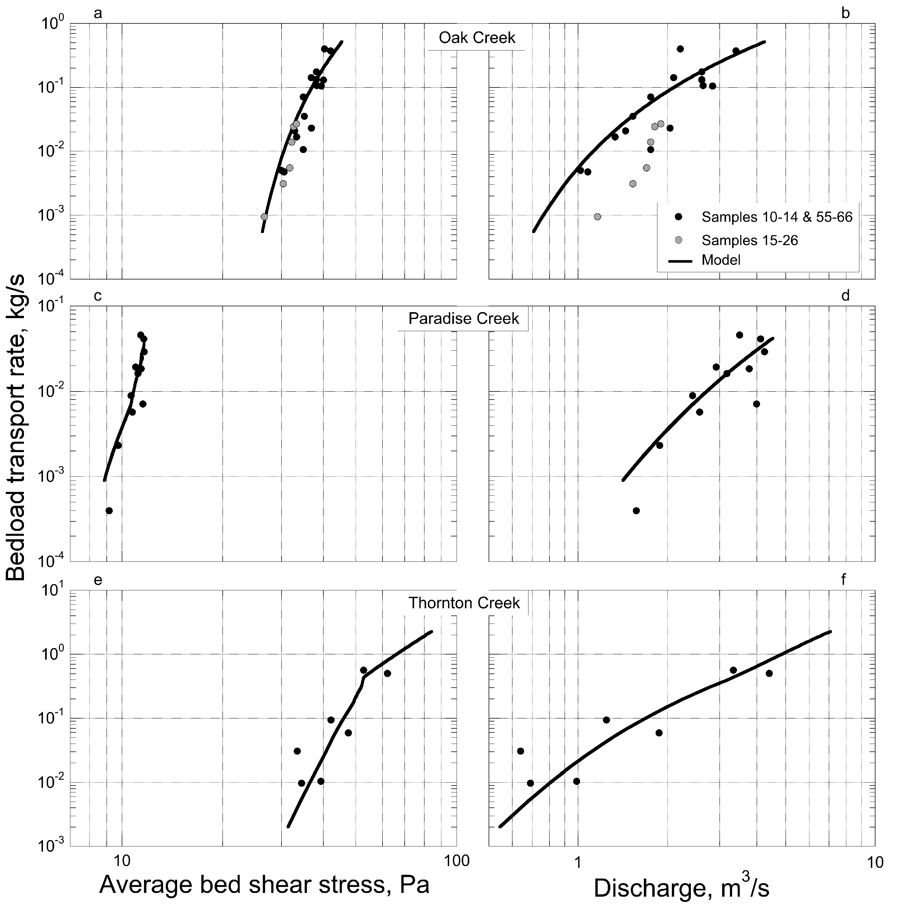
Results of model calibration for the three study sites are given in Table 1, which also summarizes site characteristics and modeling challenges. Total bedload is shown in Figure 4, using cross-section average shear stress as the independent variable. Since the use of bedload sediment rating curves is common and intuitive, we also plot the model calibrations results with water discharge as the independent variable in Figure 4.

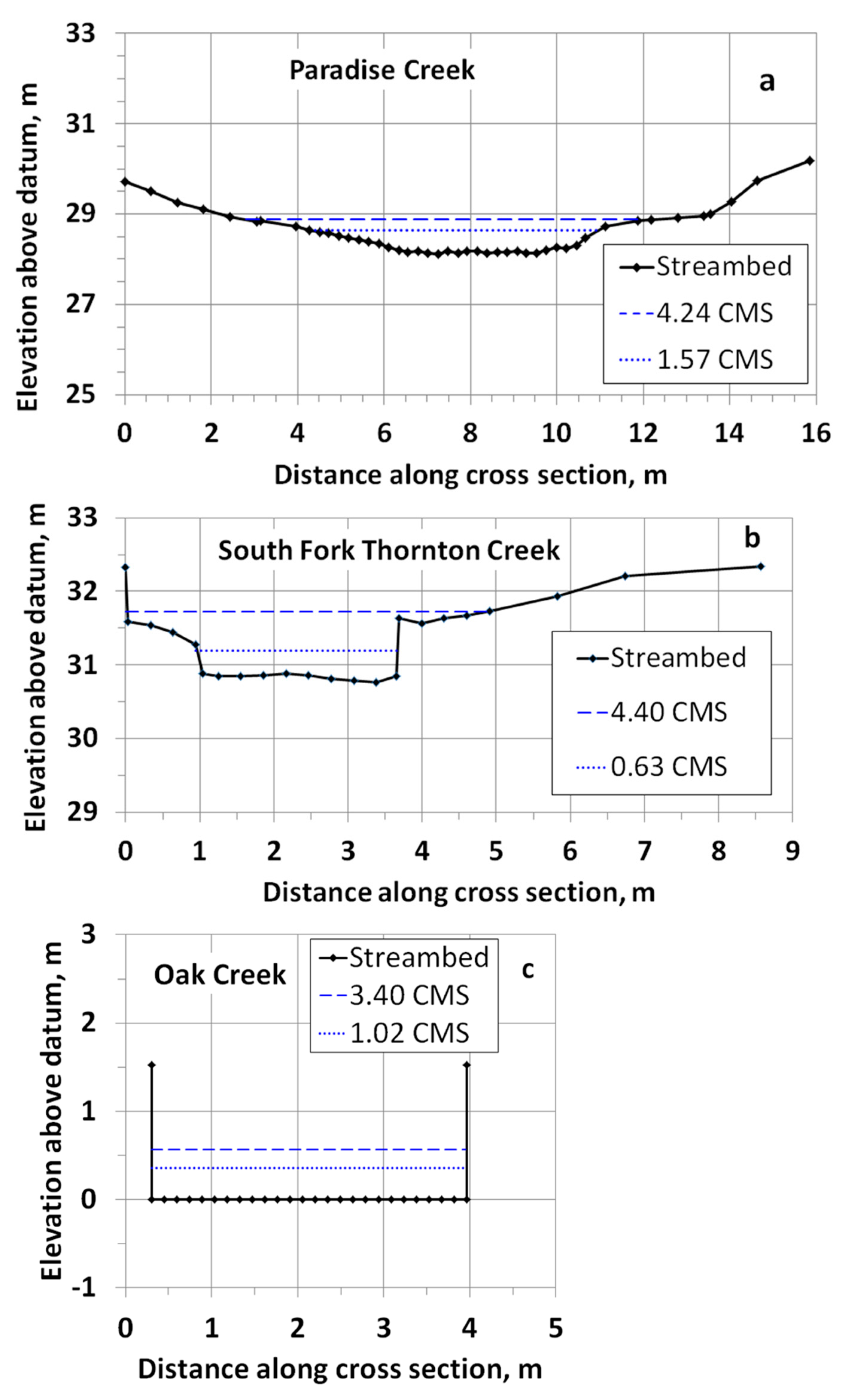
Comparison of the bedload plotted against average shear stress versus water discharge for each site reveals less scatter when shear stress is used as a predictor of bedload. This is particularly evident at Oak Creek, where six of the samples were taken during hydraulic conditions that necessitated a different water surface elevation—to discharge rating curve. Inflexions in the lines representing model-predicted bedload versus shear stress for Paradise Creek and South Fork Thornton Creek are due the fact that these lines were determined using equally-spaced intervals of water discharge, back-calculating the water surface elevation from the discharge rating curve, and then computing an average hydraulic radius and corresponding average bed shear stress. Bedload, however, was computed at each of 25 or more locations on the channel cross section using local depth to compute shear stress, and then summed to give total bedload. Since bedload increases exponentially with depth, inflexions in the cross section shape, and inflexions due to the use of a compound rating curve (necessary with overbank flow), become amplified, and total computed bedload is influenced more greatly by zones of maximum depth than by average shear stress.

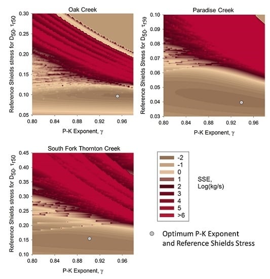
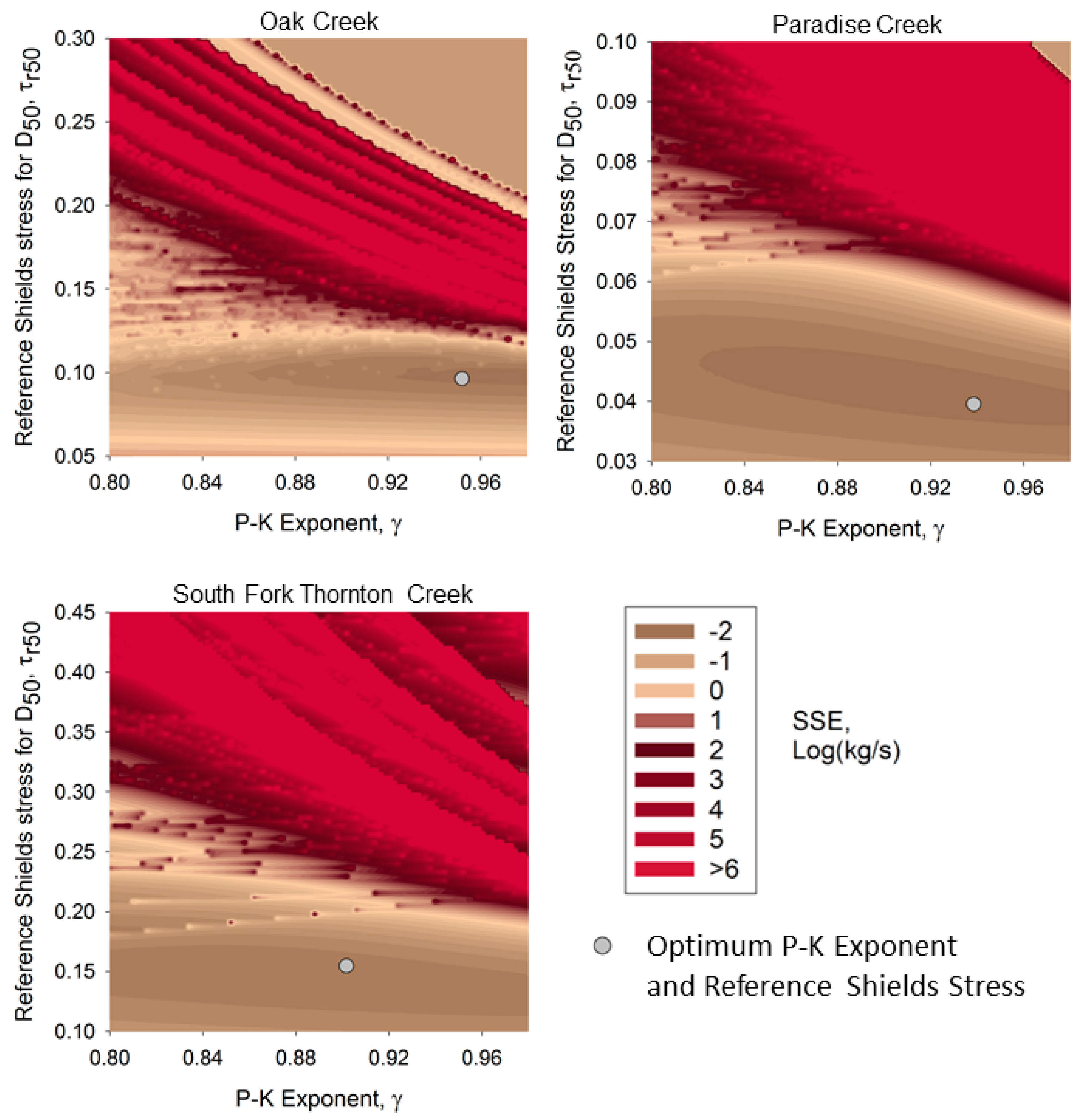
Figure 5 shows how the sum of squared error (SSE), determined from the calibrated model and calculated as the square of [log(measured load) − log(computed load)], varies with the choice of reference Shields stress (${\tau }_{r50}^{*}$) and hiding factor exponent (γ). Each grain size for each sample is included in this sum. Two observations require further explanation.

First, the use of log units equalizes the influence of large and small samples, but results in the “spiky” appearance of these graphs. The spikes in the figures represent locations in the field of ${\tau }_{r50}^{*}$ versus γ where a grain size is at the threshold of incipient motion, according to the model transport function. Since the logarithm of zero is undefined, this grain size had to be excluded from the computation of squared error. Moving slightly in either the ${\tau }_{r50}^{*}$ or γ axis direction, one reaches a location where a miniscule amount of bedload of that grain size is predicted. In logarithms, that bedload corresponds to a large negative number, resulting in the abrupt appearance of a “large” spike in SSE.

Secondly, the optimum combination of ${\tau }_{r50}^{*}$ and γ, as determined from the method described earlier using reach-averaged shear stress and total bedload for the whole cross section, does not necessarily fall on the apparent lowest SSE point in Figure 5. This is due to determination of optimum ${\tau }_{r50}^{*}$ and γ from average shear stress, while the model is computing bedload (and thus SSE) from locally-determined shear stress along the cross section.

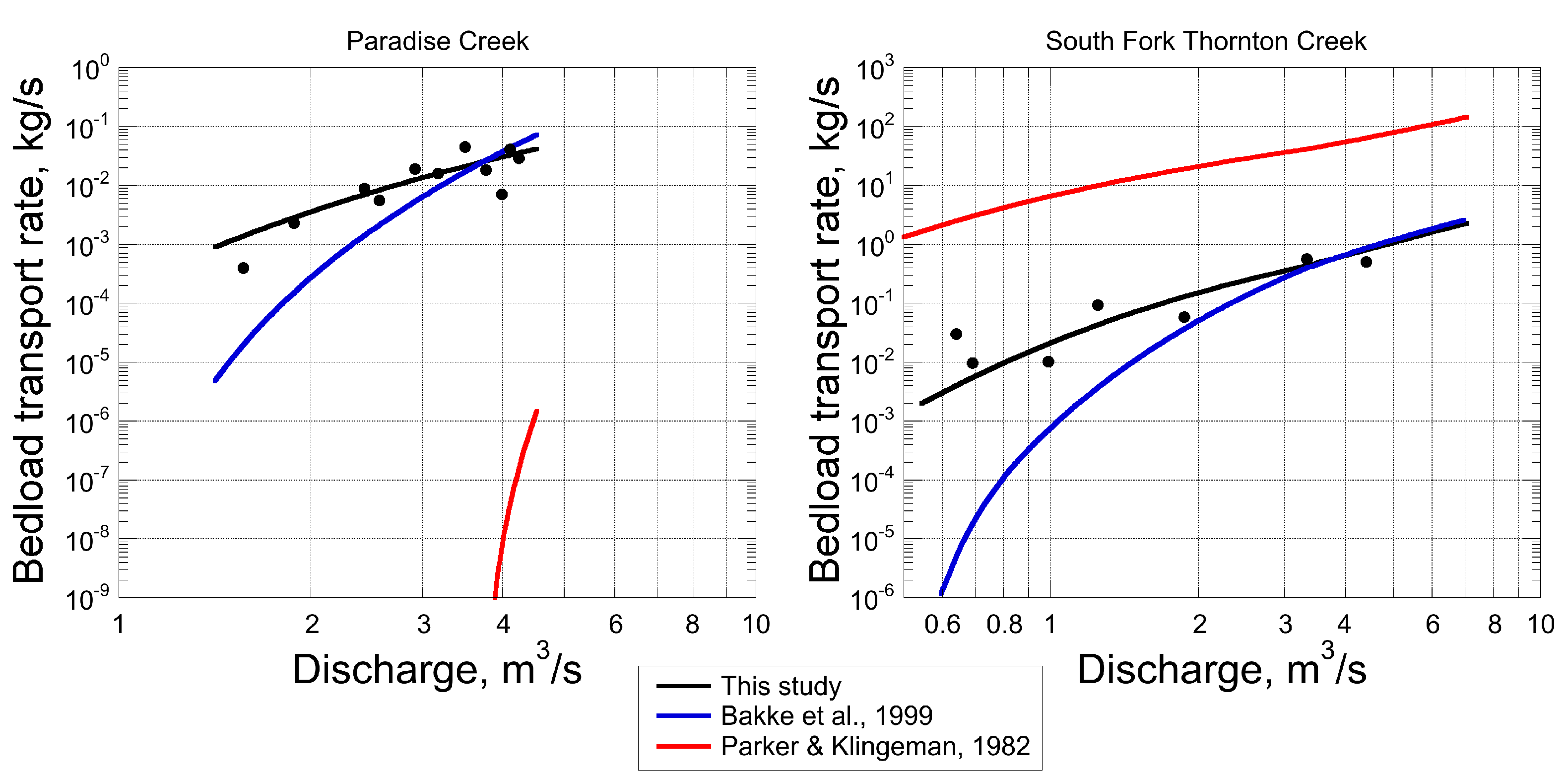
In the case of the most difficult example presented herein, South Fork Thornton Creek, the new Parker–Klingeman model calibration algorithm outperformed several similar approaches attempted (Figure 6). For example, the algorithm of Bakke, et al. [20] is calibrated by adjusting the hiding factor exponent to obtain minimum logSSE while maximizing grain movement prediction accuracy, and then adjusting the reference Shields stress (${\tau }_{r50}^{*}$) to obtain zero bias. This algorithm could be calibrated easily, but the resulting transport curve has a very large slope, and predicts unreasonably large transport rates when extrapolated to larger peaks flows, unlike the new algorithm described above. Bedload Assessment for Gravel-bed Streams (BAGS), a publicly available spreadsheet-based modeling package [21], which calibrates the Parker–Klingeman model by minimizing arithmetic SSE, would not converge to a calibrated solution for this site, probably due to the high sediment loads measured. Theoretical models, including the (uncalibrated) version of Parker–Klingeman, all yielded unreasonably high bedload transport predictions, when juxtaposed against the total annual load estimates from dredging records [27].

4. Discussion

Several modeling considerations are illustrated by these examples. Although these issues are particular to the site-calibrated modeling approach, they are inherent in the development of published theoretical models as well. In the site-calibrated approach, these considerations are explicitly addressed, which ultimately improves confidence in the results.

4.1. Optimization Using Arithmetic Loads versus Logarithms of Loads

First, development of a site- calibrated model requires choice of criteria for fitting the model to the data. One way to do this is to use a minimum average of squared errors (SSE) approach, where errors are defined as the difference between the computed and measured loads. This is the approach used in BAGS [21]. A disadvantage of using arithmetic loads to compute SSE is that the model calibration will be dominated by the larger samples. This can result in unrealistically high slopes for the load versus shear stress relationship. This can be a problem if the model is intended to be extrapolated for computation of load at large discharges, as would be the case in use for an effective discharge computation, or for computing average annual load [29]. Furthermore, for some modeling objectives, such as determining threshold discharges for grain mobilization, or predicting sediment loads or size composition under conditions of marginal transport, the smaller samples should be weighted equally to the larger samples in the modeling optimization process.

One simple way to do this, which was the procedure followed here (as well as by Bakke et al., [20]), is to compute SSE from the logarithms of loads, rather than the actual loads. However, since the logarithm of zero does not exist, combinations of model parameters that yield zero load for some of the grain samples will need to be excluded from the computation. Moreover, combinations of parameters that produce tiny amounts of predicted sediment transport will result in “spikes” in the two-dimensional surface representing SSE, since the logarithm of this tiny amount will be large and negative.

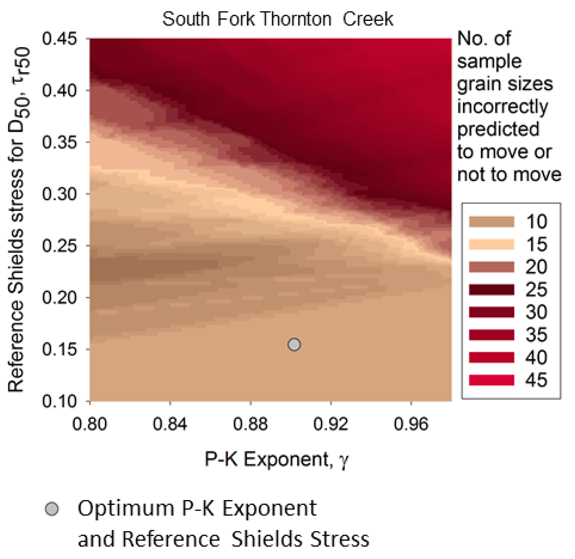
The exclusion of zero-load grain samples creates a dilemma, in that a “low” SSE region in the Figure 5 can develop due to exclusion of grain samples, rather than best model fit. Thus, another criterion, such as optimum proportion of correctly predicted movement or non-movement of sample grain sizes, or zero overall bias, needs to be added to in order to interpret the log-load SSE diagram for model best fit. As an example, Figure 7 shows grain movement prediction accuracy for South Fork Thornton Creek.

4.2. Rationale for a Two-Stage Optimization

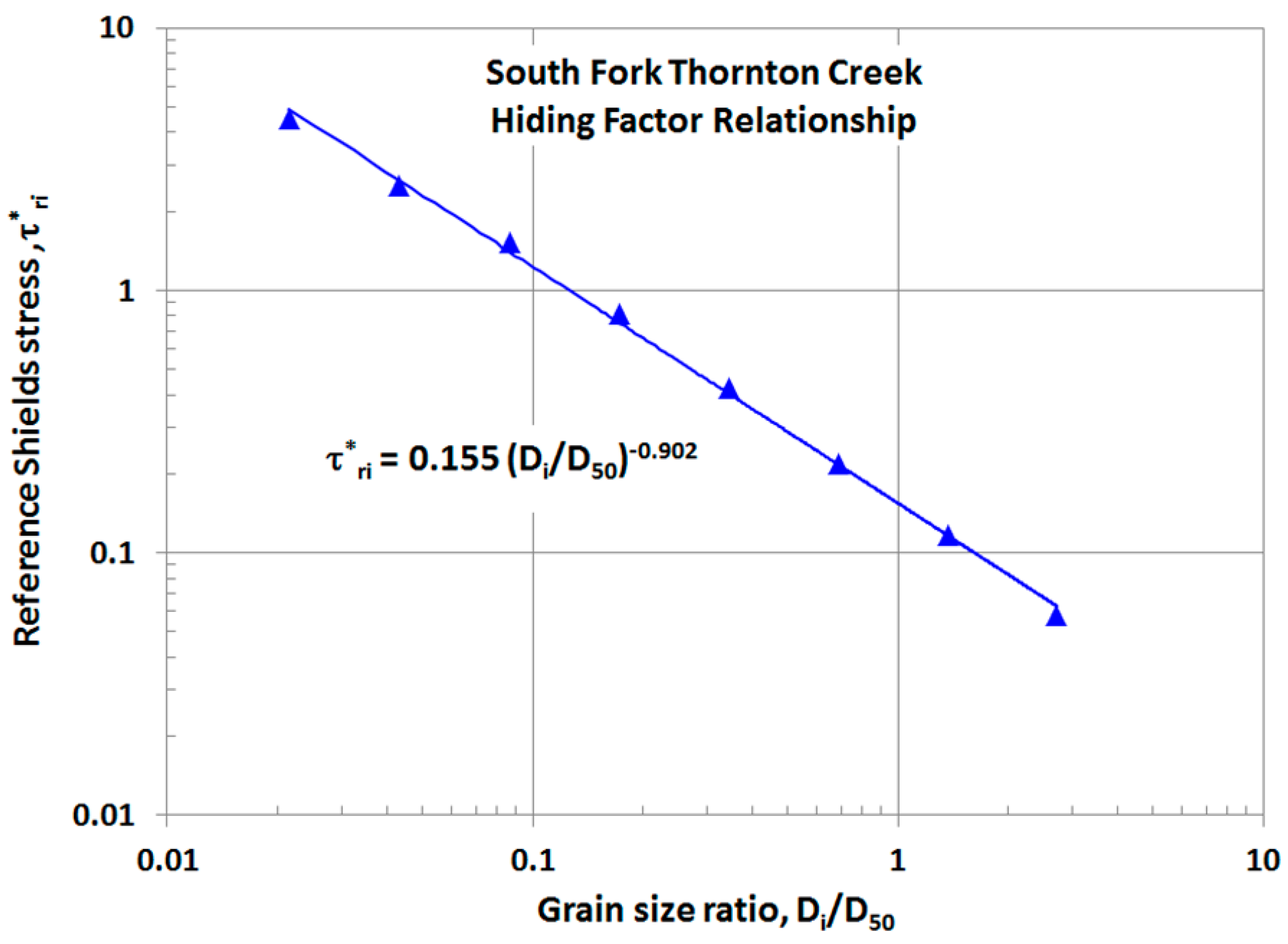
In our calibration procedure, optimization is accomplished in two steps. First, in development of the hiding factor constants ${\tau }_{r50}^{*}$ and γ, SSE in dimensionless bedload, $W_i^{*}$, and Shields stress, ${\tau }_{ri}^{*}$, are minimized to develop the regression lines used to predict ${\tau }_{ri}^{*}$. This is done in log units, but since only the (finite) bedload samples are used, there is no zero exclusion or spiking issue. Second, the transport function constant is adjusted to achieve equality between total sampled and computed bedload (zero bias). Alternatively, this could have been done with a second stage of SSE minimization, using $W_i^{*}$ versus ${\Phi }_i$, as Parker and Klingeman [3] originally did to fit the transport function curve to their data. Use of the zero-bias approach, however, is simpler. It also effectively adapts the original transport function, which was based on reach-averaged shear stress, to the quasi-two-dimensional computation being used here, which computes bedload at each point on the cross section.

4.3. One-Dimensional versus Quasi-Two-Dimensional Model Approach

Typically, sediment transport models are made one-dimensional, meaning that the sample site is represented by a single average cross section and average shear stress. This approach works well for streams like Oak Creek, which has a flume-like, rectangular cross section, but not as well for Paradise Creek, South Fork Thornton Creek or other typical alluvial streams that have a definite Thalweg. Local shear stress can be quite different in the deeper Thalweg than the cross-section average, which has implications for model prediction accuracy. A simple way to account for this is to compute shear stress and bedload using local depth rather than average hydraulic radius, and to sum the incremental bedload values over the cross section. Since the bedload transport function is highly non-linear, the difference in computed bedload using this quasi-two-dimensional approach versus a single average shear stress can be striking, and leads to optimum values for the transport function coefficient, β, which are quite different from the literature. It also results in more accurate prediction of the largest grain sizes moved for a given total bedload.

In electing to use this approach, another issue arises, however. Since the bedload samples are composites for the whole cross section, there is insufficient information to compute $W_i^{*}$ values for individual points on the cross section. Only an average $W_i^{*}$ can be computed from the data, and this requires a corresponding single (e.g., average) value of Shields stress ${\tau }_i^{*}$ for determination of the hiding factor coefficients. However, when the model computes bedload according to the transport function (Equation (6)), a local value of Shields stress is used. The result of this difference is that the bedload transport rate, $q_{Bi}$, corresponding to $W_i^{*}$ = $W_{ref}^{*}$ = 0.002, is different when computed from local depth than what its corresponding value would be when based on cross-section average shear stress in the hiding factor coefficient analysis. The second stage of the calibration process, adjusting the transport function coefficient β, eliminates this difference. Although adjustment of β could be done by another round of minimization of SSE, shifting the transport function vertically downward to pass through either the centroid of the data or to equalize the sum of total computed and measured loads is far simpler as it eliminates the complexity associated with the zero exclusion issue without affecting the fit of the curve to the data in a substantial way. Moreover, we opted to use the zero bias criterion as a way of insuring that cross sections with deep Thalwegs would not yield models that overpredict bedload at larger discharges. If predictions at marginal transport were the main objective, then an approach of adjusting β such that the transport function intersects the centroid of the data would be an appropriate choice.

4.4. Advantages of a Multi-Grain-Size Model

More generally, another issue that arises in transport modeling is which model to use, and whether to use a model that predicts total sediment volumes only, or the grain-size distribution of the bedload sediment. In regard to the data-calibrated approach described herein, two considerations are paramount.

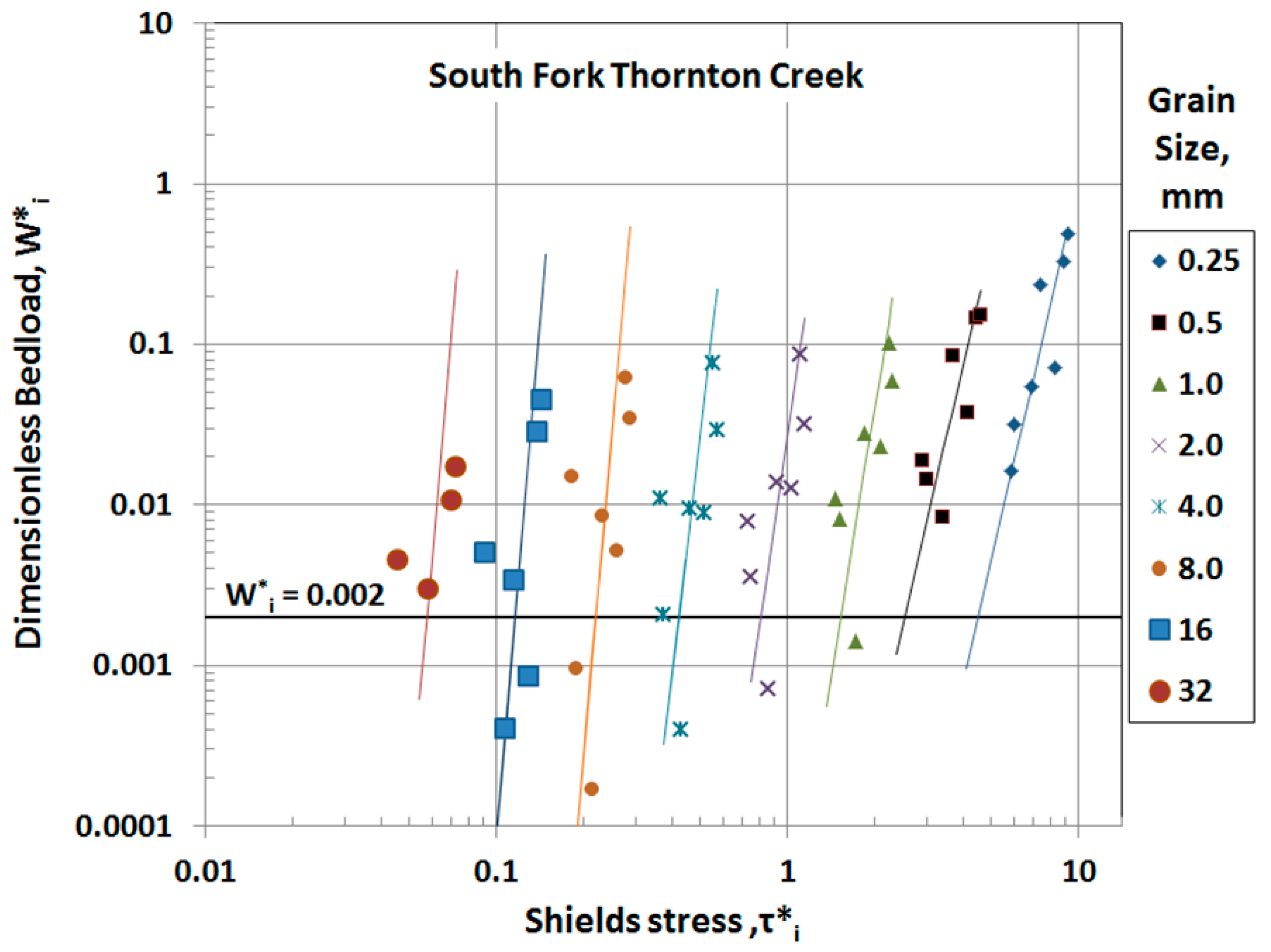
First, when only a few bedload samples are available, as was the case here with South Fork Thornton Creek, practitioners need tools for assessing data quality. One of the advantages of a multi-grain-size model is that the grain size distribution of the data contains useful information about its appropriateness for model calibration. If the site fits the assumption that the bedload approaches an equilibrium with the streambed material, which is implicit in all of the physically based models, then the data should produce a family of nearly- parallel curves such as displayed in Figure 1, and the slopes of these curves should be close to that expected for a bedload transport function, which is 4.5 in the case of the Parker–Klingeman model. The information contained in the relationship between grain sizes thus becomes part of the calibration process, which effectively expands a single bedload measurement into a sub-set of measurements, one for each grain size. This allows the practitioner to spot departures from equilibrium and, conversely, to spot irregularities in data that might suggest poor sample quality if equilibrium is expected due to other lines of evidence. The patterns visible in bedload data stratified by grain size help the modeler to diagnose whether a sample “outlier” represents a measure of the variability found in nature or, conversely, represents a sample that is deficient in some regard, and should justifiably be excluded from the calibration. An example of this departure is shown in Figure 8, for the North Fork of Thornton Creek, which was a sampling site in close proximity to the confluence with the South Fork presented above. This diagnostic power is not available when using a model that predicts only a single, average sediment volume or two components (gravel, sand), as opposed to a series of multiple grain sizes.

Finally, although most any model can, in principle, be calibrated with bedload data, the most state-of-the-art gravel transport models incorporate some form of a “hiding factor” to account for the way that the structure of the streambed causes particle mobility by grain size to adjust over what it would be in a streambed of uniform-sized particles, and thereby to achieve equilibrium between the streambed material and the bedload in transport [3]. Without this hiding factor, which effectively increases the apparent mobility of larger particles and reduces that of smaller particles, a model will invariably over-predict transport of small grain sizes and under-predict the large sizes, and typically will over-predict the total sediment load [22]. Moreover, a site-calibrated model should incorporate a transport function whose form derives from basic physical principles, ensuring consistency with the body of work under which the original model was derived.

5. Conclusions

We have shown that predicting bedload sediment flux using site-calibration of a bedload transport model can achieve high accuracy using only a small number of flux measurements. In particular, we developed a new algorithm for site calibration of the Parker–Klingeman (1982) model, which predicts bedload flux by particle size class. The approach is applied in three study sites representing a spectrum of hydraulic complexity and data availability, and is shown to be especially well suited to streams with high sediment loads, and to applications where extrapolation of the predicted sediment rating curve is required. Key elements underlying the success of this approach include: log-transformation of sediment loads to optimize the model for minimum error; accounting for lateral variation in shear stress; and the use of a multi-grain-size model, which maximizes the information value of each flux measurement, and by including a ‘hiding function’, accounts for the dynamics of particle interactions that govern the stress-flux relationship. Finally, we provided a novel graphical depiction of the calibration process, to assist practitioners in understanding and applying the site calibration technique.

References

1. Wilcock, P.R.; Pitlick, J.; Cui, Y. Sediment Transport Primer: Estimating Bed-Material Transport in Gravel-Bed Rivers; General Technical Report RMRS-GTR-226; U.S. Department of Agriculture, Forest Service, Rocky Mountain Research Station: Fort Collins, CO, USA, 2009.
2. Bunte, K.; Abt, S.R. Sampling Surface and Subsurface Particle-Size Distributions in Wadable Gravel-and Cobble-Bed Streams for Analyses in Sediment Transport, Hydraulics, and Streambed Monitoring; General Technical Report RMRS-GTR-74; U.S. Department of Agriculture, Forest Service, Rocky Mountain Research Station: Fort Collins, CO, USA, 2001.
3. Parker, G.; Klingeman, P.C. On why gravel bed streams are paved. Water Resour. Res. 1982, 18, 1409–1423. [Google Scholar] [CrossRef]
4. Bagnold, R.A. An empirical correlation of bedload transport rates in flumes and natural rivers. Proc. R. Soc. A 1980, 372, 453–473. [Google Scholar] [CrossRef]
5. Meyer-Peter, E.; Muller, R. Formulas for bed-load transport. In Proceedings of the 2nd Meeting of the International Association for Hydraulic Structures Research, International Association of Hydraulic Research, Delft, The Netherlands, 7 June 1948; pp. 39–64. [Google Scholar]
6. Brownlie, W.R. Prediction of Flow Depth and Sediment Discharge in Open Channels; General Technical Report KH-R-43A; W.M. Keck Laboratory of Hydraulics and Water Resources, California Institute of Technology: Pasadena, CA, USA, 1981. [Google Scholar]
7. Buffington, J.M.; Montgomery, D.R. A systematic analysis of eight decades of incipient motion studies, with special reference to gravel-bedded rivers. Water Resour. Res. 1997, 33, 1993–2029. [Google Scholar] [CrossRef]
8. Andrews, E.D. Entrainment of gravel from naturally sorted riverbed material. Geol. Soc. Am. Bull. 1983, 94, 1225–1231. [Google Scholar] [CrossRef]
9. Parker, G.; Toro-Escobar, C.M. Equal mobility of gravel in streams: The remains of the day. Water Resour. Res. 2002, 38, 1264. [Google Scholar] [CrossRef]
10. Parker, G.; Klingeman, P.C.; McLean, D.G. Bedload and size distribution in paved gravel-bed streams. J. Hydr. Div. 1982, 108, 544–571. [Google Scholar] [CrossRef]
11. Parker, G. Surface-based bedload transport relation for gravel rivers. J. Hydr. Res. 1990, 28, 417–436. [Google Scholar] [CrossRef]
12. Wilcock, P.R.; Crowe, J.C. Surface-based transport model for mixed-size sediment. J. Hydr. Eng. 2003, 129, 120–128. [Google Scholar] [CrossRef]
13. Barry, J.J.; Buffington, J.M.; King, J.G. A general power equation for predicting bed load transport rates in gravel bed rivers. Water Resour. Res. 2004, 40, W10401. [Google Scholar] [CrossRef]
14. Barry, J.J.; Buffington, J.M.; King, J.G. Correction to A general power equation for predicting bed load transport rates in gravel bed rivers. Water Resour. Res. 2007, 43, W08702. [Google Scholar] [CrossRef]
15. Emmett, W.W. Quantification of channel-maintenance flows for gravel-bed rivers. In Wildland Hydrology; Olsen, D.S., Potyondy, J.P., Eds.; American Water Resources Association: Herndon, VA, USA, 1999; pp. 77–84. [Google Scholar]
16. Ryan, S.E.; Emmett, W.W. The Nature of Flow and Sediment Movement in Little Granite Creek near Bondurant, Wyoming; General Technical Report RMRS-GTR-90; U.S. Department of Agriculture, Forest Service, Rocky Mountain Research Station: Ogden, UT, USA, 2002.
17. Segura, C.; Pitlick, J. Coupling fluvial-hydraulic models to predict gravel transport in spatially variable flows. J. Geophys. Res. Earth Sci. 2015, 120, 834–855. [Google Scholar] [CrossRef]
18. Monsalve, A.; Yager, E.M.; Turowski, J.M.; Rickenmann, D. A probabilistic formulation of bed load transport to include spatial variability of flow and grain size distributions. Water Resour. Res. 2016, 52, 3579–3598. [Google Scholar] [CrossRef]
19. Wilcock, P.R. Toward a practical method for estimating sediment-transport rates in gravel-bed rivers. Earth Surf. Proc. Landf. 2001, 26, 1395–1408. [Google Scholar] [CrossRef]
20. Bakke, P.D.; Basdekas, P.O.; Dawdy, D.R.; Klingeman, P.C. Calibrated Parker-Klingeman model for gravel transport. J. Hydrol. Eng. 1999, 125, 657–660. [Google Scholar] [CrossRef]
21. Pitlick, J.; Cui, Y.; Wilcock, P. Manual for Computing Bedload Transport Using BAGS (Bedload Assessment for Gravel-Bed Streams) Software; General Technical Report RMRS-GTR-223; U.S. Department of Agriculture, Forest Service, Rocky Mountain Research Station: Fort Collins, CO, USA, 2009.
22. Dawdy, D.R.; Wang, W.C. Prediction of gravel bedload transport with SAM. In Water Policy and Management: Solving the Problems, Proceedings of the 21st Annual Conference, Water Resources Planning Division, ASCE, Denver, CO, USA, 23–26 May 1994; Fontane, D.G., Ed.; ASCE: Reston, VA, USA, 1994; pp. 420–424. [Google Scholar]
23. Cheng, C.-L.; Van Ness, J.W. Statistical Regression with Measurement Error; Arnold: London, UK, 1999; pp. 16–17. [Google Scholar]
24. Milhous, R.T. Sediment Transport in a Gravel-Bottomed Stream. Ph.D. Dissertation, Department of Civil Engineering, Oregon State University, Corvallis, OR, USA, 1973. [Google Scholar]
25. Klingeman, P.C. Sediment Transport Facilities, Oak Creek, Oregon; Oak Creek Sediment Transport Report F1; Water Resources Research Institute, Oregon State University: Corvallis, OR, USA, 1979. [Google Scholar]
26. Katz, S.B. Sediment Transport Modeling and Implications for Benthic Primary Producers in Oak Creek, OR. Master’s Thesis, Science in Water Resources Engineering, Oregon State University, Corvallis, OR, USA, 2016, unpublished. [Google Scholar]
27. Bakke, P.D. Characterization and Review of Sediment Transport Modeling and Field Data Collection in Thornton Creek; Unpublished Report; Seattle Public Utilities: Seattle, WA, USA; U.S. Fish and Wildlife Service: Lacey, WA, USA, 27 August 2012.
28. Perkins, S. Geomorphic Evaluation for 10718 35th Avenue NE Sedimentation Pond on Thornton Creek. Perkins Geosciences; Unpublished Report; Seattle Public Utilities and Otak, Inc.: Seattle, WA, USA, June 2003.
29. Doyle, M.W.; Shields, D.; Boyd, K.F.; Skidmore, P.B.; Dominick, D.-W. Channel-forming discharge selection in river restoration design. J. Hydrol. Eng. 2007, 133, 831–837. [Google Scholar] [CrossRef]
Figure 1. Size-specific transport rates. Log-log (power) regression lines are fit to the data for each grain size class to determine the size-specific reference Shields stress, τ r i * , the value of τ i * where the fit line crosses W i * = 0.002. Regressions are computed to minimize sum of squared distances between the points and the regression line (orthogonal regression), except for the 32 mm line, which had too few points to accurately determine its slope. It was assigned a slope equal to the average of the 16 mm and 8 mm slopes, and was constrained to pass through the centroid of the data.
Water 09 00441 g001
Figure 2. Hiding factor equation. Reference Shields stress, τ r i * , for each grain size, determined from the intersection of the regression lines shown in Figure 1 with W i * = 0.002, are plotted against the grain size ratio Di/D50 to obtain the hiding factor relationship. Here, D50 refers to the subsurface layer. τ r 50 * is found to be 0.155, and the exponent is 0.902.
Water 09 00441 g002
Figure 3. Channel cross sections used in the model. Also shown are water surface elevations for the greatest and smallest sample discharges, in m3/s.
Water 09 00441 g003
Figure 4. Total bedload transport versus cross-section average bed shear stress (left) and versus discharge (right). (a,b) are Oak Creek, Oregon (Milhouse, 1973). All samples shown, taken during the winter of 1971 at discharges greater than 1 m3/s, were used for calibration. Site hydraulics were different for the 6 samples shown in grey, which required use of a separate equation relating water surface elevation to discharge. These samples were used in calibration but are not well described by the model curve when displayed against discharge. (c,d) are Paradise Creek, Oregon. (e,f) are South Fork Thornton Creek, Seattle, Washington. Inflexions of the Paradise Creek and South Fork Thornton Creek model curves are due to inflexions in channel cross section and use of multiple water-level to discharge rating equations.
Water 09 00441 g004
Figure 5. Average sum of squared error (SSE). SSE was computed by application of the Parker–Klingeman (1982) model to Oak Creek, Paradise Creek, and South Fork Thornton Creek for combinations of hiding factor reference Shields stress for D50 and exponent (see Equation (1)) as shown. SSE is computed from all grain sizes, of all samples, in which both measured and computed load are non-zero. Values of optimum reference Shield stress and exponent are given in Table 1.
Water 09 00441 g005
Figure 6. Total bedload transport versus discharge. The site-calibrated model described in this study (black line) is contrasted against the method of Bakke et al. [20] (blue line) and use of the original values of the hiding factor equation constants from Parker and Klingeman [3] without calibration (red line). Paradise Creek, shown on the left, has relatively low shear stress during bedload transporting events compared to the South Fork Thornton Creek, on the right, resulting in a striking difference between uncalibrated versus calibrated model performance.
Water 09 00441 g006
Figure 7. Grain movement prediction error for South Fork Thornton Creek. Prediction error is the count of all grain sizes, in all samples, where the model predicted sediment movement when none was measured, or where sediment was measured but none was predicted. Smaller numbers signify greater accuracy in predicting grain movement. There were a total of 52 measurements by grain size in the seven available bedload samples.
Water 09 00441 g007
Figure 8. Dimensionless bedload versus Shields stress for the North Fork Thornton Creek. Samples marked with open circles are not consistent with the rest of the data due to differing site hydraulics, and were eliminated from the calibration process. This example is provided to show how the multi-grain-size modeling approach can be used to check data quality and sediment equilibrium assumptions.
Water 09 00441 g008