An Investigation into the Effects of Temperature Gradient on the Soil Water–Salt Transfer with Evaporation

Abstract

Temperature gradients exist in the field under brackish water irrigation conditions, especially in northern semi–arid areas of China. Although there are many investigators dedicated to studying the mechanism of brackish water irrigation and the effect of brackish water irrigation on crops, there are fewer investigations of the effects of temperature gradient on the water–salt transport. Based on the combination of a physical experiment and a mathematical model, this study was conducted to: (a) build a physical model and observe the redistribution of soil water–heat–salt transfer; (b) develop a mathematical model focused on the influence of a temperature gradient on soil water and salt redistribution based on the physical model and validate the proposed model using the measured data; and (c) analyze the effects of the temperature gradient on the soil water–salt transport by comparing the proposed model with the traditional water–salt model in which the effects of temperature gradient on the soil water–salt transfer are neglected. Results show that the soil temperature gradient has a definite influence on the soil water–salt migration. Moreover, the effect of temperature gradient on salt migration was greater than that of water movement.

1. Introduction

Freshwater resources are relatively limited [1], but groundwater (or seawater) resources are abundant in many countries or regions [2]. Therefore, the rational use of groundwater resources is an important approach to solve water resource crises [3,4]. Research shows that brackish water irrigation is propitious to crop quality in a certain range of salinity [5,6]. In an agricultural system that involves brackish water irrigation, an interaction occurs between salt and water in the soil [7]. A soil temperature gradient exists in the irrigation system, thereby affecting the transfer of soil water by influencing the physical properties of soil moisture (e.g., surface tension, viscosity coefficient of soil moisture, etc.) [8,9], as well as its state and structure [10]. Soil moisture is a medium of heat and mass transfer, and can induce heat and salt migration. Soil water movement can lead to a new salt concentration and temperature gradient [11]; therefore, the effects of temperature gradient on soil water and salt transport cannot be disregarded [12].

Saline water irrigation was carried out in soil with a clay interlayer, and the law of water and salt transport in soil was studied [13]. There have been several studies on the effects of brackish water irrigation on different crops during a growth period and the effects of saline water on the soil water and salt distribution [14,15,16,17]. However, these studies have mainly focused on studying the distribution of soil water and salt transport in brackish water irrigation, thus neglecting the effects of temperature gradient on the redistribution of water and salt.

The effects of saline irrigation on soil water–heat–salt variation and cotton yield and quality have been studied [18], and the degree of salt stress damage on cotton was weakened by reducing the evaporation of soil, thus increasing the soil temperature and inhibiting the accumulation of salt in the film mulching condition [19]. These studies revealed that soil salt transfer was affected by soil moisture and temperature during salt water irrigation. However, the effects of temperature gradient on the soil water–salt transfer were not considered in these studies.

In general, the infiltration process is very complex. Many studies have built models to accurately study the entire process of infiltration through many experiments and theoretical analysis [20,21,22]. The SWAP model was used to simulate water and salt transport under different conditions of brackish water irrigation. Additionally, reasonable irrigation methods and systems were developed in References [23,24]. The Salt model was used to discuss the effect of irrigation salinity on soil salinity [25]. However, the effects of temperature on water and salt transfer in these models was also neglected.

A model tool was needed to accurately study the effect of temperature on the soil water–salt transfer. As a widely used numerical simulation software, HYDRUS–1D has been used by many previous studies [26,27,28]. However, there were three key challenges during the formulation of the model. The first challenge was that although soil water movement in a partially saturated porous medium has been described by a modified form of the Richards equation, water flow due to thermal gradients was neglected. Second, despite solute transfer being described by partial differential equations governing one-dimensional nonequilibrium during transient water flow in a variably saturated rigid porous medium, the effects of temperature gradient on the solute transfer has not been considered. Finally, our last challenge was that we could not obtain and rewrite the original code due to its commercial nature.

In summary, there are some limitations to the previous studies. First, most experiments focused on the distribution of soil water and salt transport in brackish water irrigation; however, the influence of temperature gradient on the water movement and salt migration were ignored. Second, in some previous water–salt transfer models, the heat flux equation was not considered. Finally, in the water movement and salt migration equations, the soil water movement and salt migration attributed to thermal gradients (e.g., the moisture diffusivity and the salt diffusivity under the influence of temperature gradient) have been neglected in some soil water–heat–salt transfer models such as HYDRUS–1D. Therefore, these studies could not clearly indicate the effects of temperature gradient on soil water–salt transfer.

In the proposed model, to study the effects of temperature gradient on water movement and salt migration, water movement and salt migration equations were improved by adding the moisture diffusivity and the solute diffusion coefficient under the influence of temperature gradient, respectively. The aims of this study were to (a) build a physical model of the non-isothermal vertical soil column in the laboratory; (b) observe the redistribution of the water–heat–salt transfer; (c) develop a mathematical model focused on the influence of temperature gradient on soil water and salt redistribution based on the physical model; (d) validate the proposed model by the measured data and analyze the accuracy of the model; and (e) analyze the effects of temperature gradient on soil water–salt transport by comparing the proposed model with the traditional water–salt model where the effects of temperature gradient on soil water–salt transfer was neglected.

2. Materials and Methods

The topsoil layer (0–20 cm) is located on the land surface, and is easily affected by changes in the external environment. In the soil layer, the high organic matter and soil microorganism contents, as well as the concentrated root distribution substantially affects farm crops. Therefore, study of the relationship among moisture, heat, and salt in the topsoil is important for reasonable irrigation and fertilizer applications. A vertical short soil column was used in this study, and the coupling transportation of moisture, heat, and salt was simulated.

Soil samples were collected from the cultivated land of the Taigu County Fruit Tree Research Institute in Shanxi Province, China. The surface soil is a silty (sandy) loam, and was homogeneous. The main physical parameters of the undisturbed soil included bulk density and field moisture capacity with values of 1.47 g·cm⁻³ and 0.25 cm³·cm⁻³, respectively. The undisturbed soil was retrieved for the laboratory and characterized by soil stratification, as well as dried, ground, and mixed.

Vertical soil columns with sealed bottoms and inner diameters and lengths of 8 cm and 30 cm, respectively, were used in this study. Uniform perforation was arranged on the soil column used to insert the temperature sensor. The soil column was filled with layers of soil with bulk density. The waterhead was controlled using a Martensite tube. The heating device was placed above the soil column. Sodium chloride solution was selected as the irrigation salt solution in the experiment. The amount and concentration of the three levels (i.e., W1, W2, and W3) were 295 mL, 2.39 g·L⁻¹; 236 mL, 3.00 g·L⁻¹; and 177 mL, 4.01 g·L⁻¹, respectively. The temperature of each soil layer was measured using a multi-way soil temperature tester. Soil moisture content was determined using the drying method. The salt concentration of the soil solution was determined using a DDSJ–308A conductivity meter. Data were recorded once every 1 h during the observation period. The depth profiles for measuring a variable (e.g., soil water content, temperature, and salt content) were 0, 2, 4, 6, 8, 10, 12, 14, 16, 18, and 20 cm. Figure 1 shows the test equipment.

3. Methods

3.1. Description of the Soil Water–Salt Model with Thermal Gradient

Assuming that the soil is homogeneous and isotropic, the soil skeleton does not expand nor shrink. The transfer of water–heat–salt in soil mainly occurs in the vertical direction; therefore, it is considered a one–dimensional problem. The effect of gas phase on the soil was ignored, and local thermodynamic equilibrium conditions were assumed.

3.1.1. Water Movement Equation

Soil is a typical porous medium. In porous media, the motion of fluid satisfies Darcy’s Law. The movement of soil moisture is driven by soil water potential; that is, soil moisture spontaneously moves from the region of high soil water potential to a region of low soil water potential. Moreover, the movement and changes in matter follow the principle of mass conservation. The mass conservation principle is applied as a continuity equation for fluid motion in porous media. In view of the effect of soil temperature gradient on the physical properties of soil moisture, the equation for water movement under the influence of a temperature gradient can be established according to Richards equation and continuity equation.

$$\frac{\partial \mathsf{\theta }}{\partial \mathrm{t}}=\frac{\partial }{\partial \mathrm{z}}\left[\mathrm{D}\left(\mathsf{\theta }\right)\frac{\partial \mathsf{\theta }}{\partial \mathrm{z}}\right]+\frac{\partial }{\partial \mathrm{z}}\left[{\mathrm{D}}_{\mathrm{T}}\frac{\partial \mathrm{T}}{\partial \mathrm{z}}\right]-\frac{\partial \mathrm{K}\left(\mathsf{\theta }\right)}{\partial \mathrm{z}}$$

(1)

where $\mathsf{\theta }$ is the soil water content (cm³·cm⁻³); z is the spatial coordinates (in a downward direction) (cm); t is the time (min); T is the temperature (change with time t and spatial coordinate z) (°C); D($\mathsf{\theta }$) is the unsaturated soil water diffusivity (cm²·min⁻¹); D_T is the moisture diffusivity under the influence of temperature gradient.

3.1.2. Heat Flux Equation of Soil

Soil water movement affects the transformation of soil heat, and heat flow in the soil follows Fourier’s Law. The system follows the law of conservation of energy, and an equation for heat flux influenced by flow can be established.

$$\frac{\partial \mathrm{T}}{\partial \mathrm{t}}=\frac{1}{{\mathrm{C}}_{\mathrm{v}}}*\frac{\partial }{\partial \mathrm{z}}\left[{\mathrm{K}}_{\mathrm{h}}\frac{\partial \mathrm{T}}{\partial \mathrm{z}}\right]+\left\{\frac{\partial {\mathrm{D}}_{\mathrm{h}}}{\partial \mathrm{z}}+\frac{{\mathsf{\rho }}_{\mathrm{w}}{\mathrm{c}}_{\mathrm{w}}}{{\mathrm{C}}_{\mathrm{v}}}*\left[-\mathrm{D}\left(\mathsf{\theta }\right)*\frac{\partial \mathsf{\theta }}{\partial \mathrm{z}}+\frac{\mathrm{K}\left(\mathsf{\theta }\right)}{\partial \mathrm{z}}\right]\right\}*\frac{\partial \mathrm{T}}{\partial \mathrm{z}}$$

(2)

where C_v is the soil volumetric heat capacity (J·cm⁻³·°C⁻¹); K_h is the soil thermal conductivity (10⁻³ J·cm⁻¹·°C⁻¹); D_h is the soil thermal diffusivity (10⁻³ cm²·min⁻¹); ${\mathsf{\rho }}_{\mathrm{w}}$ is the soil water density (g·cm⁻³); C_w is the volumetric heat capacity of soil water (J·cm⁻³·°C⁻¹); K($\mathsf{\theta }$) is the unsaturated soil water conductivity (cm·min⁻¹).

3.1.3. Salt Solution Migration Equation of Soil

Soil moisture is a medium of heat and mass transfer, and can induce heat and salt migration. Solution migration is an immensely complicated phenomenon. First, soil moisture is a medium of salt solution transfer and can induce salt migration. Second, the solute solution migrates from a high concentration to a low concentration gradient when a certain concentration gradient is present in the soil. Finally, the solute enters a small gap from a large gap, and from a small space into an even smaller space in the soil salt solution migration. Therefore, the effect of temperature gradient on the solution migration in the soil cannot be neglected. The equation for soil salt solution migration with soil temperature gradient can be established based on the law of conservation of mass.

$$\frac{\partial \left(\mathsf{\theta }\mathrm{c}\right)}{\partial \mathrm{t}}=\frac{\partial }{\partial \mathrm{z}}\left[{\mathrm{D}}_{\mathrm{sh}}\frac{\partial \mathrm{c}}{\partial \mathrm{z}}\right]+\frac{\partial }{\partial \mathrm{z}}\left[{\mathrm{D}}_{\mathrm{TM}}\frac{\partial \mathrm{T}}{\partial \mathrm{z}}\right]-\frac{\partial \left(\mathrm{qc}\right)}{\partial \mathrm{z}}$$

(3)

where c is the soil solution concentration (g·kg⁻¹); D_sh is the hydrodynamic dispersion coefficient; D_TM is the diffusion coefficient of the solute with temperature gradient; and q is the soil moisture flux.

Equations for coupled soil water–heat–salt transfer consist of Equations (1)–(3). The mathematical model for the coupled soil water–heat–salt transfer can be established when the initial and boundary conditions are given.

3.1.4. Initial and Boundary Conditions

The initial conditions of the soil water, temperature, and salt concentration at each discretization node in the study area at the beginning of the simulation are expressed as follows:

$$\mathsf{\theta }\left(\mathrm{z},\mathrm{t}=0\right)={\mathsf{\theta }}_0\left(\mathrm{z}\right)0\le \mathrm{z}\le 20\mathrm{cm}$$

(4)

$$\mathrm{T}\left(\mathrm{z},\mathrm{t}=0\right)={\mathrm{T}}_0\left(\mathrm{z}\right)0\le \mathrm{z}\le 20\mathrm{cm}$$

(5)

$$\mathrm{c}\left(\mathrm{z},\mathrm{t}=0\right)={\mathrm{c}}_0\left(\mathrm{z}\right)0\le \mathrm{z}\le 20\mathrm{cm}$$

(6)

where z is the depth of soil (cm); t is the time (min); ${\mathsf{\theta }}_0\left(\mathrm{z}\right)$, ${\mathrm{T}}_0\left(\mathrm{z}\right)$, and ${\mathrm{c}}_0\left(\mathrm{z}\right)$ are obtained by field observation, whilst values at the nodes without field data are obtained by quadratic interpolation method.

The top boundary conditions of the soil water movement and heat flux are the Neumann conditions based on the laws of mass and energy conservation, as follows:

$$-\mathrm{D}\left(\mathsf{\theta }\right)\frac{\partial \mathsf{\theta }}{\partial \mathrm{z}}+\mathrm{K}\left(\mathsf{\theta }\right)=-\mathrm{E}\left(\mathrm{t}\right)\mathrm{z}=0,\mathrm{t}>0$$

(7)

$$-{\mathrm{K}}_{\mathrm{h}}\frac{\partial \mathrm{T}}{\partial \mathrm{z}}=\mathrm{G}\left(\mathrm{t}\right)\mathrm{z}=0,\mathrm{t}>0$$

(8)

The soil moisture evaporation intensity is E(t). Moreover, q (0, t), E(t), and J (0, t) follow the relationship: q (0, t) = −E(t); J (0, t) = 0. The top boundary condition of the salt concentration is the Cauchy boundary condition, as follows:

$${\mathrm{D}}_{\mathrm{sh}}\frac{\partial \mathrm{c}}{\partial \mathrm{z}}+\mathrm{E}\left(\mathrm{t}\right)\mathrm{c}\left(0,\mathrm{t}\right)=0\mathrm{z}=0,\mathrm{t}>0$$

(9)

The bottom boundary conditions are the zero-Neumann conditions. The bottom boundary conditions are described as follows:

$$\frac{\partial \mathsf{\theta }}{\partial \mathrm{z}}=0\mathrm{z}=20\mathrm{cm}\mathrm{t}\ge 0$$

(10)

$$\frac{\partial \mathrm{T}}{\partial \mathrm{z}}=0\mathrm{z}=20\mathrm{cm}\mathrm{t}\ge 0$$

(11)

$$\frac{\partial \mathrm{c}}{\partial \mathrm{z}}=0\mathrm{z}=20\mathrm{cm}\mathrm{t}\ge 0$$

(12)

where E (t) is the surface soil evaporation intensity (cm·min⁻¹); G (t) is surface heat flux (W·cm⁻²); q (0, t) and J (0, t) are the water flux and salt solute flux, respectively, with time at the top of the soil column.

3.2. Description of the Traditional Water–Salt Model Without Thermal Gradient

3.2.1. The Governing Equations

The water movement equation of the traditional water–salt model (without thermal gradient) can be established according to Richards equation and continuity equation.

$$\frac{\partial \mathsf{\theta }}{\partial \mathrm{t}}=\frac{\partial }{\partial \mathrm{z}}\left[\mathrm{D}\left(\mathsf{\theta }\right)\frac{\partial \mathsf{\theta }}{\partial \mathrm{z}}\right]-\frac{\partial \mathrm{K}\left(\mathsf{\theta }\right)}{\partial \mathrm{z}}$$

(13)

The salt solution migration equation of the traditional water–salt model (without thermal gradient) can be established based on the law of conservation of mass.

$$\frac{\partial \left(\mathsf{\theta }\mathrm{c}\right)}{\partial \mathrm{t}}=\frac{\partial }{\partial \mathrm{z}}\left[{\mathrm{D}}_{\mathrm{sh}}\frac{\partial \mathrm{c}}{\partial \mathrm{z}}\right]-\frac{\partial \left(\mathrm{qc}\right)}{\partial \mathrm{z}}$$

(14)

3.2.2. Initial and Boundary Conditions

The initial of the traditional water–salt model without thermal gradient can be described as Equations (4) and (6). The top boundary conditions are described as Equations (7) and (9), and the bottom boundary conditions are followed as Equations (10) and (12).

3.3. Determination of Model Parameters

3.3.1. Determination of the Parameters for Soil Water Movement

The relationship between the soil water content and pressure head proposed by van Genuchten [29] is adopted as follows:

$$\mathsf{\theta }\left(\mathrm{h}\right)={\mathsf{\theta }}_{\mathrm{r}}+\frac{\left({\mathsf{\theta }}_{\mathrm{s}}-{\mathsf{\theta }}_{\mathrm{r}}\right)}{{\left[1+{\left(\mathsf{\alpha }\left|\mathrm{h}\right|\right)}^{{\mathrm{n}}_0}\right]}^{\mathrm{m}}}$$

(15)

The van Genuchten (VG) equation is applied to determine the unsaturated hydraulic conductivity of soil. The unsaturated hydraulic conductivity can be determined from the characteristic curve of soil water and from the saturated hydraulic conductivity, as follows:

$$\mathrm{K}\left(\mathrm{h}\right)={\mathrm{K}}_{\mathrm{s}}{\mathrm{S}}_{\mathrm{e}}^{\frac{1}{2}}[1-(1-{\mathrm{S}}_{\mathrm{e}}^{\frac{1}{\mathrm{m}}}{)}^{\mathrm{m}}{]}^2$$

(16)

where ${\mathsf{\theta }}_{\mathrm{s}}$ and ${\mathsf{\theta }}_{\mathrm{r}}$ are saturated and residual values of the soil water content (cm³·cm⁻³), respectively; m and n0 are shape parameters following the relationship m = 1 − 1/n₀, and $\mathsf{\alpha }$ (m⁻¹) is a scaling parameter of the matric potential; K_s is the saturated hydraulic conductivity of soil (cm·min⁻¹); S_e, ${\mathsf{\theta }}_{\mathrm{s}}$, and ${\mathsf{\theta }}_{\mathrm{r}}$ follow the relationship:

$${\mathrm{S}}_{\mathrm{e}}=\frac{\mathsf{\theta }-{\mathsf{\theta }}_{\mathrm{r}}}{{\mathsf{\theta }}_{\mathrm{s}}-{\mathsf{\theta }}_{\mathrm{r}}}$$

(17)

In this study, the characteristic curve of soil water and the saturated hydraulic conductivity were measured by pressure membrane and permeability meter, respectively. Parameters $\mathsf{\alpha },{\mathrm{n}}_0,{\mathsf{\theta }}_{\mathrm{s}},{\mathsf{\theta }}_{\mathrm{r}}$ are obtained as detailed in the model calibration below.

Table 1. The physical parameters of the soil.

Depth (cm)	$\mathsf{\gamma }$ (g·cm−3)	${\mathsf{\theta }}_{\mathbf{f}}$ (cm3·cm−3)	${\mathsf{\theta }}_{\mathbf{s}}$ (cm3·cm−3)	${\mathsf{\theta }}_{\mathbf{r}}$ (cm3·cm−3)	$\mathsf{\alpha }$	${\mathbf{n}}_{\mathbf{0}}$
0–20	1.470	0.250	0.350	0.022	0.024	2.030

shows the physical parameters of the soil.

The presence of a temperature gradient alters the moisture diffusion rate D_T. An empirical formula of temperature gradient was used to describe the effect of temperature on water content as follows [30]:

$$\mathrm{q}=-\mathrm{D}\left(\mathsf{\theta }\right)\frac{\partial \mathsf{\theta }}{\partial \mathrm{x}}-{\mathrm{D}}_{\mathrm{T}}\frac{\partial \mathrm{T}}{\partial \mathrm{x}}$$

(18)

The explicit differential equation method was used to separate the equation. According to the estimation from observed data (i.e., the water content and temperature of different sections at different times) in the laboratory test, the discrete equation was solved by programming.

Therefore, D_T is a function of temperature T:

$${\mathrm{D}}_{\mathrm{T}}=3.6*{10}^{-14.012}*{\mathrm{T}}^{6.9146}$$

(19)

The water balance method was used to calculate soil evaporation, according to the irrigation experiment standard [31]. Soil evaporation can be calculated by the following equation:

$$\mathrm{ET}={\displaystyle \sum }_{\mathrm{i}=1}^{\mathrm{N}}{\mathrm{H}}_{\mathrm{i}}\left({\mathrm{W}}_{\mathrm{i}1}-{\mathrm{W}}_{\mathrm{i}2}\right)+\mathrm{M}+\mathrm{P}+\mathrm{K}-\mathrm{D}$$

(20)

where ET is the farmland evapotranspiration during the calculation period (cm); i is the number of soil layer; N is the total number of total soil layers; H_i is the soil thickness of the layer i (cm); W_i1 is the initial soil moisture content of layer i (cm³·cm⁻³); W_i2 is the end soil moisture content of layer i (cm³·cm⁻³); M is the irrigation amount during the calculation period (cm); P is the rainfall during the calculation period (cm); K is the groundwater recharge during the calculation period (cm); and D is the water discharge during the calculation period (cm).

Given that one end of the soil column was sealed with a plastic cloth, then K = 0. Given that the water holding capacity of root layer is larger, then D = 0.

3.3.2. Determination of the Parameters for Soil Heat Transfer

Soil thermal properties mainly include soil heat capacity (C_v), soil thermal conductivity (K_h), and soil thermal diffusivity (D_h). The relationship among the three is as follows:

$${\mathrm{K}}_{\mathrm{h}}={\mathrm{C}}_{\mathrm{v}}*{\mathrm{D}}_{\mathrm{h}}$$

(21)

Soil heat capacity C_v can be calculated as follows:

$${\mathrm{C}}_{\mathrm{v}}={\mathsf{\theta }}_{\mathrm{s}}{\mathrm{C}}_{\mathrm{s}}+{\mathsf{\theta }}_{\mathrm{w}}{\mathrm{C}}_{\mathrm{w}}+{\mathsf{\theta }}_{\mathrm{a}}{\mathrm{C}}_{\mathrm{a}}$$

(22)

where $\mathsf{\theta }$_s, $\mathsf{\theta }$_w, and $\mathsf{\theta }$_a are the volume of solid matter, water, and gas, respectively, in a unit volume of soil. C_s, C_w, and C_a are the heat capacity of solid matter, water, and gas, respectively.

The unsteady state method was used to calculate soil thermal diffusivity by conducting the horizontal soil column experiment in the laboratory [32].

K_h represents the thermal conductivity of the soil, and is mainly determined from the soil moisture, soil texture, and gaps in the soil. The thermal conductivity can be obtained after having determined soil heat capacity and diffusivity by Equation (21). The relationship between the K_h and water content is as follows:

$${\mathrm{K}}_{\mathrm{h}}=45.318*{\mathsf{\theta }}^{0.6619}$$

(23)

3.3.3. Determination of the Parameters for Soil Salt Solution Migration

Sodium chloride solutions are relatively stable and can be transported without chemical reaction. Therefore, the horizontal soil column method [33] was used to measure the hydrodynamic dispersion coefficient of the unsaturated soil when the water body was not considered. The value of the longitudinal dispersion coefficient was 0.99.

The diffusion coefficient of the solute can be affected by temperature gradient. An empirical formula of temperature was used to describe the effect of temperature gradient on the soil salt migration as follows [34]:

$$\mathrm{J}=-{\mathsf{\theta }\mathrm{D}}_{\mathrm{sh}}\frac{\partial \mathrm{c}}{\partial \mathrm{x}}+\mathrm{qc}-{\mathrm{D}}_{\mathrm{TM}}\frac{\partial \mathrm{T}}{\partial \mathrm{x}}$$

(24)

where J is the soil solute flux (mol·m⁻²s⁻¹).

The explicit differential equation method was used to separate this equation. The discrete equation was solved after the estimations were obtained from the observed data in the laboratory test, such as water content, temperature, and the salt content of different sections at different times. Moreover, D_TM is a function of temperature T:

$${\mathrm{D}}_{\mathrm{TM}}=1.175*{10}^{-7}*{\mathrm{T}}^{2.7766}$$

(25)

3.4. Modeling Strategy

3.4.1. Calibration

The implicit difference and central difference methods were used to discretize the governing equations. The water movement, heat flux, and salt solution migration equations were solved with an iterative Newton–Raphson technique. Before the model could be used to simulate, the relevant parameters had to be determined. The parameters $\mathsf{\alpha },{\mathrm{n}}_0,{\mathsf{\theta }}_{\mathrm{r}},{\mathrm{and}\mathsf{\theta }}_{\mathrm{s}}$, which were used to compute the unsaturated soil water conductivity of the soil, were determined in the calibration process. The least square method was used to establish the objective functions, and the objective function is expressed as follows:

$$\min \mathrm{f}={\displaystyle \sum }_{\mathrm{i}=1}^{\mathrm{N}}{\left({\mathsf{\theta }}_{\mathrm{i}}-\mathsf{\theta }\left({\mathrm{h}}_{\mathrm{i}},\mathrm{X}\right)\right)}^2$$

(26)

where ${\mathsf{\theta }}_{\mathrm{i}}$ is the measured water content in sample i in the experiment of the characteristic curve for soil water (cm³·cm⁻³); ${\mathrm{h}}_{\mathrm{i}}$ is the soil water potential corresponding the measured water content (cm); $\mathsf{\theta }\left({\mathrm{h}}_{\mathrm{i}},\mathrm{X}\right)$ is the soil water content calculated by Equation (15); X is the parameter vector (${\mathsf{\theta }}_{\mathrm{r}},{\mathsf{\theta }}_{\mathrm{s}},\mathsf{\alpha },\mathrm{n}$), which will be determined; N is the number of measured point samples.

A hybrid genetic algorithm [35] was employed to optimize these parameters in this study, because determining them manually would have been a tedious job. The optimized parameters are listed in Table 1.

The incremental time step $\mathrm{∆}\mathrm{t}$ and spatial step $\mathrm{∆}\mathrm{z}$ adopted were 1 (min) and 0.01 (m), respectively. The tolerant differential errors of h, T, and c between any two consecutive computational times were 0.01 (cm) H₂O, 0.01 (°C), and 0.01 (g·kg⁻¹) at the steady state, respectively. Moreover, tolerances ${\mathsf{\epsilon }}_{\mathrm{h}},{\mathsf{\epsilon }}_{\mathrm{T}},{\mathrm{and}\mathsf{\epsilon }}_{\mathrm{c}}$ of h, T, and c were 0.1 (cm) H₂O, 0.1 (°C), and 0.1 (g·kg⁻¹), respectively, to prevent the occurrence of any undesirable numerical instability during the modeling process.

To further test the accuracy of the simulation results obtained using the proposed model, the simulated soil moisture content, temperature, and salinity were compared with the measured values. Mean absolute error (MAE) and root mean square error (RMSE) were used as criteria for evaluating the model [36]. The MAE values were estimated as:

$$\mathrm{MAE}=\frac{1}{\mathrm{N}}{\displaystyle \sum }_{\mathrm{i}=1}^{\mathrm{N}}\left({\mathrm{y}}_{\mathrm{i}}-{\mathrm{x}}_{\mathrm{i}}\right)$$

(27)

and RMSE values were estimated as [37]:

$$\mathrm{RMSE}=\sqrt{\frac{{{\displaystyle \sum }}_{\mathrm{i}=1}^{\mathrm{N}}{\left[\frac{{\mathrm{y}}_{\mathrm{i}}-{\mathrm{x}}_{\mathrm{i}}}{{\mathrm{x}}_{\mathrm{i}}}\right]}^2}{\mathrm{N}}}\times 100\%$$

(28)

where N is the number of observed point samples for the variable; y_i is the predicted value of a variable (the water content, temperature, and salinity); x_i is the observed values of a variable (the water content, temperature, and salinity).

3.4.2. Validation/Prediction

Based on the calibrated model, profiles of soil water content, temperature, and salinity were simulated. As the initial values of the model, the soil water content, temperature, and salt content of the soil were measured one hour after irrigation. Simulations were carried out in three phases: Phase 1 (from 0–60 min), Phase 2 (from 0–180 min), and Phase 3 (from 0–1440 min). Moreover, simulations were carried out under two conditions: Condition 1 and Condition 2. Under Condition 1, the temperature gradient was considered in the water–salt transfer model (in fact, this was a coupled water–heat–salt transport model); and under Condition 2, the temperature gradient was ignored in the water–salt transfer model, which consisted of the water movement and salt transfer equations without temperature gradient.

4. Results and Discussion

4.1. Simulation Results and Analysis

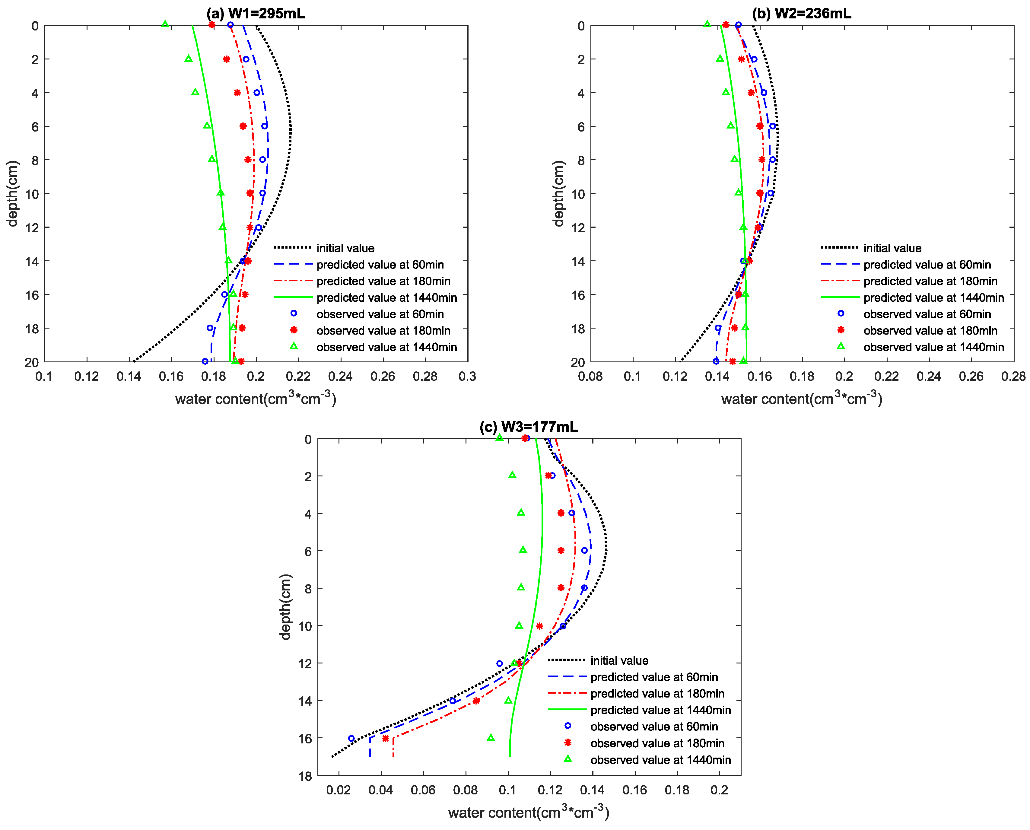
Figure 2a,b show that the simulated values of soil water content first increased (peaked near 6–8 cm deep) with soil depth, and decreased eventually in Phases 1 and 2. This was due to the lower viscosity and tension of soil water with considerably higher soil temperature in the upper soil column than the lower soil column. Thereafter, the soil water movement was faster in the higher layers of the soil column than in the lower layers. The soil water accumulated in the middle layer; however, the simulated values of the soil water content increased gradually with soil depth in Phase 3. This was mainly due to the sealed bottom that caused the soil water to accumulate at the bottom of the column. The difference (shown in Figure 2c) was that the simulated values of the soil water content first increased (peaked near 6–8 cm deep) with soil depth, and decreased eventually in all phases.

There were significant differences in the decrease of soil water content on the soil surface under different irrigation conditions. These differences followed the W1 > W2 > W3 pattern. This was mainly because the greater the irrigation amount, the greater the evaporation intensity of the soil surface [38]. In this study, the average evaporation intensity at the W1 level was 1.08 times and 1.66 times greater than that of W2 and W3 levels, respectively.

Under different irrigation treatments, the simulated curves of the water content showed roughly the same trend with time and soil depth. At <13 cm deep, soil water content gradually decreased with time as cumulative evaporation was greater with time in the upper soil layer; thus, soil water potential decreased, and the subsoil water moved upwards. Therefore, the evapotranspiration of the soil could continue; however, some soil water moved downwards due to the gravitational potential. The maximum amplitude reduction of the soil water content was at the peak during the whole simulated period. At levels W1, W2, and W3, the amplitude reduction of the soil water content was 0.0371 cm³·cm⁻³, 0.0186 cm³·cm⁻³, and 0.0298 cm³·cm⁻³, respectively, during the whole simulated period. Moreover, the decrease rate of soil water at the peak decreased with time. In Phase 1, at levels of W1, W2, and W3, the decrease rate of soil water at the peak was 1.83 × 10⁻⁴ cm³·cm⁻³·min⁻¹, 0.633 × 10⁻⁴ cm³·cm⁻³·min⁻¹, and 1.13 × 10⁻⁴ cm³·cm⁻³·min⁻¹, respectively. However, at levels W1, W2, and W3 in Phase 3, the decrease rate of soil water at the peak was 2.57 × 10⁻⁵ cm³·cm⁻³·min⁻¹, 1.29 × 10⁻⁵ cm³·cm⁻³·min⁻¹, and 2.06 × 10⁻⁵ cm³·cm⁻³·min⁻¹, respectively. At >13 cm deep, soil water content gradually increased with time, mainly from the accumulated soil water accumulated at the bottom of the column due to the sealed base. The maximum increase amplitude of the soil water content was at the bottom of the soil column during the whole simulated period. During the whole simulated period, at levels W1, W2, and W3, the increase amplitude of the soil water content was 0.0457 cm³·cm⁻³, 0.0312 cm³·cm⁻³, and 0.0840 cm³·cm⁻³, respectively. Moreover, there was an increased rate of soil water at the bottom over time, with an increase rate of soil water at the bottom of 6.11 × 10⁻⁴ cm³·cm⁻³·min⁻¹, 2.83 × 10⁻⁴ cm³·cm⁻³·min⁻¹, and 3.00 × 10⁻⁴ cm³·cm⁻³·min⁻¹, respectively, at levels W1, W2, and W3 in Phase 1. However, in Phase 3 at levels W1, W2, and W3, the decrease rate of soil water at the bottom was 3.17 × 10⁻⁵ cm³·cm⁻³·min⁻¹, 2.16 × 10⁻⁵ cm³·cm⁻³·min⁻¹, and 5.83 × 10⁻⁵ cm³·cm⁻³·min⁻¹, respectively.

A comparison of Figure 2a–c shows that the simulated accuracy of water content at level W3 was lower than that of levels W1 and W2. This was mainly from the enlarged effect of vapor on soil water movement due to less soil water content and more soil voids with less irrigation [39,40].

Figure 3a–c show that under different irrigation treatments, the simulated curves of the soil temperature showed roughly the same trend with time and soil depth. Additionally, they showed that soil temperature decreased with soil depth, and the difference between the upper and lower soil layer temperature decreased with time. This was mainly due to the application of a heat device above the soil column before the start of the experiment, and the removal of the heat device after the start of the experiment had commenced.

At <4 cm deep, the soil temperature decreased obviously in Phase 1. The amplitude reduction of soil temperature on the surface followed the W1 > W2 > W3 pattern, which was 2.81 °C, 2.09 °C, and 2.05 °C, respectively. This was mainly because the soil column heat transported from the inside to outside due to the removal of the heat device at the beginning of the experiment; whereas in the initial stage of the experiment, evaporation at the W1 level was 1.03 times and 1.07 times greater than that of the W2 and W3 levels, respectively. Therefore, the greater the evaporation, the more energy dissipated [41,42]. At >4 cm deep, the soil temperature increased gradually with time. Moreover, the increase amplitude of the soil temperature was largest at 6–8 cm deep.

After 60 min, at <9 cm deep, the soil temperature decreased with time. The maximum amplitude reduction of the soil temperature was on the surface during the whole simulated period. At levels W1, W2, and W3, the amplitude reduction of the soil temperature was 3.2 °C, 2.37 °C, and 2.33 °C, respectively; moreover, the decrease rate of the soil temperature decreased with time. In Phase 2 at levels W1, W2, and W3, the decrease rate of soil temperature on the surface was 0.016 °C·min⁻¹, 0.012 °C·min⁻¹, and 0.012 °C·min⁻¹, respectively. However, in Phase 3 (at levels W1, W2, and W3), the decrease rate of soil temperature on the surface was 0.0022 °C·min⁻¹, 0.0017 °C·min⁻¹, and 0.0016 °C·min⁻¹, respectively. At >9 cm deep, the soil temperature increased with time, and the maximum increase amplitude of the soil temperature was at the bottom, which was 0.32 °C, 0.36 °C, and 0.43 °C, respectively, during the whole simulated period. Furthermore, the increase rate of soil temperature decreased with time. At the Phase 2 levels W1, W2, and W3, the increase rate of soil temperature at the bottom was 0.0007 °C·min⁻¹, 0.0009 °C·min⁻¹, and 0.0018 °C·min⁻¹, respectively. However, in Phase 3, at levels W1, W2, and W3, the increase rate of soil temperature at the bottom was 0.00020 °C·min⁻¹, 0.00025 °C·min⁻¹, and 0.00029 °C·min⁻¹, respectively.

These results showed that at the same depth and time interval, the increase of soil temperature followed a W1 < W2 < W3 pattern. This was mainly due to the fact that the greater the irrigation amount, the greater the soil water content in the soil column, thus, in the process of soil redistribution, the increase in soil temperature with a higher water content was smaller because of the larger heat capacity of water than soil [43].

Figure 4a,b show that the simulated values of soil salt content first increased (peaked near 6–8 cm deep) with soil depth before decreasing. This trend was similar to the trend of soil water content with soil depth, mainly because a larger water content meant that more salt would be carried in the process of migration.

There were significant differences in the decrease of soil salt content on the soil surface under different irrigation conditions. These differences followed the W1 < W2 < W3 pattern, where the more soil water decreased, the more salt content increased. In this study, the evaporation intensity on the soil surface was the highest [42].

Under different irrigation treatments, the simulated curves of the soil salt content showed roughly the same trend with time and soil depth. At <3 cm deep, the salt content decreased with time in Phases 1 and 2, but increased with time in Phase 3.

At 3 cm < z < 13 cm deep, the soil salt content decreased with time given that the solute transport was based on soil water, and the soil water content of the lower layer increased due to the downward movement of soil water by gravity in the process of soil water redistribution. The maximum increase amplitude of the soil salt content was at the peak during the whole simulated period. At levels W1, W2, and W3, the increase amplitude of the soil salt content was 0.0332 g·kg⁻¹, 0.0284 g·kg⁻¹, and 0.0472 g·kg⁻¹, respectively, during the whole simulated period. Moreover, the increase rate of soil salt content at the peak decreased with time. In Phase 1 at levels W1, W2, and W3, the increase rate of soil salt content at the peak was 2.31 × 10⁻⁴ g·kg⁻¹·min⁻¹, 1.93 × 10⁻⁴ g·kg⁻¹·min⁻¹, and 2.86 × 10⁻⁴ g·kg⁻¹·min⁻¹, respectively. However, in Phase 3, the increase rate of soil salt content at the peak was 2.30 × 10⁻⁵ g·kg⁻¹·min⁻¹, 1.97 × 10⁻⁵ g·kg⁻¹·min⁻¹, and 3.27 × 10⁻⁵ g·kg⁻¹·min⁻¹ for levels W1, W2, and W3, respectively. Given that the soil temperature was the highest at the top of soil column, water conductivity increased due to less viscous force and surface tension. In the process of downward migration, the solubility of soil salinity decreased with soil depth, as the lower soil temperature was lower than the upper soil temperature. Thus, the soil salt accumulated, and the salt molecule had a certain effect on water absorption [19], which made the soil water and salt of the lower soil layer migrate upward. Therefore, the salt content increased in the middle of the soil column.

At >13 cm deep, the soil salt content decreased with time. The maximum amplitude reduction of the soil temperature was at the bottom during the whole simulated period. Moreover, the decrease rate of the soil salt content decreased with time. In Phase 1 at levels W1, W2, and W3, the decrease rate of soil salt content at the bottom was 1.53 × 10⁻⁴ g·kg⁻¹·min⁻¹, 0.85 × 10⁻⁴ g·kg⁻¹·min⁻¹, and 0.71 × 10⁻⁴ g·kg⁻¹·min⁻¹, respectively. However, at levels W1, W2, and W3 in Phase 3, the decrease rate of soil salt content at the bottom was 0.49 × 10⁻⁵ g·kg⁻¹·min⁻¹, 1.07 × 10⁻⁵ g·kg⁻¹·min⁻¹, and 4.43 × 10⁻⁵ g·kg⁻¹·min⁻¹, respectively.

Compared with Figure 4a–c, at level W1, the soil salt content increased with time in Phases 2 and 3. This was mainly because there was more evaporation on the soil surface at the level W1 than at levels W2 and W3, which made the soil water decrease and the soil salt content increase slightly at the bottom.

4.2. Error Analysis of Simulated and Observed values

The relative and absolute errors of the simulated and observed values for soil water content, temperature, and salt content under the different conditions in the three phases were calculated, and the results are shown in

Table 2. Error between the simulated and observed values for soil water content under the different conditions.

Phase		Condition One			Condition Two
		W1	W2	W3	W1	W2	W3
One	MAE	0.0014	0.0023	0.0056	0.0021	0.0027	0.0085
	RMSE	1.02	1.45	12.53	1.64	1.96	16.91
Two	MAE	0.0019	0.0036	0.0060	-	-	-
	RMSE	1.56	2.31	6.80	-	-	-
Three	MAE	0.0021	0.0033	0.0091	0.0041	0.0052	0.0131
	RMSE	1.95	2.91	9.91	3.14	4.08	13.19

MAE is the mean absolute error, (cm³·cm⁻³); RMSE is the root mean square error, (%).

,

Table 3. Error between the simulated and observed values for soil temperature under the different conditions.

Phase		Condition One			Condition Two
		W1	W2	W3	W1	W2	W3
One	MAE	0.1476	0.0523	0.0653	-	-	-
	RMSE	1.05	0.20	0.23	-	-	-
Two	MAE	0.0421	0.0638	0.0399	-	-	-
	RMSE	0.16	0.24	0.16	-	-	-
Three	MAE	0.0384	0.0438	0.0597	-	-	-
	RMSE	0.17	0.19	0.22	-	-	-

MAE is the mean absolute error, (°C); RMSE is the root mean square error, (%).

and

Table 4. Error between the simulated and observed values for soil salt content under the different conditions.

Phase		Condition One			Condition Two
		W1	W2			W1	W2
One	MAE	0.0042	0.0059	0.0067	0.0061	0.0067	0.0118
	RMSE	6.35	9.37	17.62	15.24	15.88	48.61
Two	MAE	0.0042	0.0045	0.0069	-	-	-
	RMSE	6.99	8.62	20.11	-	-	-
Three	MAE	0.0041	0.0066	0.0089	0.0074	0.0079	0.0139
	RMSE	4.32	10.09	20.54	13.09	15.81	43.25

MAE is the mean absolute error, (g·kg⁻¹); RMSE is the root mean square error, (%).

.

By using the proposed mathematical calculation for soil water–heat–salt transfer, Table 2, Table 3 and Table 4 demonstrate the high accuracy of the simulation results in the soil column for the changed dynamic in simulating soil moisture, temperature, and salt content, respectively.

4.3. Sensitivity Analysis

Given the effects of temperature gradient on water movement and salt migration, the simulated curves of the water content, temperature, and salt content were obtained under the two conditions, and are shown in Figure 5 and Figure 6.

Figure 5a–f show that regardless of whether the effects of temperature gradient on the water–salt transfer were considered, the simulated curves of water content showed roughly the same trend in Phase 1. Figure 5a,c,e show that the simulated values of water content under Condition 1 were smaller than those of Condition 2. This was because the effect of temperature gradient on soil water movement could be realized based on affecting moisture diffusivity. The moisture diffusivity increased due to the temperature gradient, and the speed of soil water movement downward was accelerated by moisture diffusivity. In addition, the differences between the simulated values of water content under both conditions decreased with soil depth because the soil temperature was highest and temperature gradient was largest on the topsoil, and decreased with soil depth. At levels W1, W2, and W3, the moisture diffusivity of the top (under the influence of temperature gradient) was 1.57 times, 1.42 times, and 1.33 times greater than that of the bottom during this period, respectively.

Figure 5b,d,f show that at levels W1 and W2, the simulated values of soil water content increased with soil depth; however, the simulated values of soil water content decreased with soil depth at level W3. The simulated values of soil water content under Condition 1 were smaller than that of Condition 2. Moreover, the differences between the simulated values of water content under both conditions decreased with a decrease in irrigation amount because at the end of the experiment, the temperature of the upper and lower soil layers reached a constant value. Additionally, moisture diffusivity under the influence of temperature gradient at level W1 were 1.17 times and 1.44 times greater than that of conditions W2 and W3, respectively. Therefore, moisture diffusivity under the influence of temperature gradient and the differences between the simulated values under both conditions decreased with a decrease in irrigation amount.

Figure 6a–f show that there was a great difference in the salt migration regardless of whether the temperature gradient was considered. At <3 cm deep, the simulated values of soil salt content under both conditions increased with soil depth; however, the simulated values under Condition 2 were obviously smaller than that of Condition 1. At levels W1, W2, and W3, the simulated values of soil salt content on the topsoil under condition one were 0.0491 g·kg⁻¹, 0.0509 g·kg⁻¹, and 0.0793 g·kg⁻¹, respectively, which were smaller than that of Condition 2. These indicate that the difference between the simulated value of the soil salt content under both conditions increased with a decrease in irrigation amount, mainly because the effect of temperature gradient on soil salt migration was realized based on affected solute diffusivity. Solute diffusivity increased with the higher temperature on the topsoil before the downward speed of the soil salt transfer increased. Therefore, compared with Condition 2 (where the temperature gradient was ignored), the simulated values of soil salt content were smaller under Condition 1. The difference between the simulated values under both conditions decreased with the decrease in irrigation amount as at level W3, solute diffusivity under the influence of temperature gradient was 1.12 times and 1.26 times greater than that of levels W1 and W2, respectively.

Under both conditions at >3 cm deep, the simulated values of soil salt content were the first to increase (peaked near 6–8 cm deep) with soil depth, before gradually decreasing. However, the simulated values under Condition 1 were significantly greater than those of Condition 2 (at 6–8 cm deep, the difference between the simulated values under both conditions was the largest). Moreover, the difference between the simulated values under both conditions decreased with soil depth because the speed of soil salt transfer under Condition 1 was greater than that of Condition 2 due to the effect of temperature gradient on solute diffusivity. Additionally, at levels W1, W2, and W3, the average solute diffusivity of the topsoil was 19.65%, 18.74%, and 18.65%, respectively, which were higher than that of the bottom layer. These results indicated that solute diffusivity decreased with soil depth due to a decreasing temperature gradient. This resulted in the accumulation of salt in the lower layer, and the accumulation of soil salt content under Condition 1 was greater than that of Condition 2. The influence of soil temperature on solute diffusivity decreased due to the decreasing temperature gradient with soil depth. Therefore, the difference between the simulated values under both conditions decreased with soil depth through solute diffusivity.

To study the effect of temperature on soil water–salt transfer more clearly, the error between the simulated and observed values for soil water content and salt content under both conditions are shown in Table 2 and Table 4.

Table 2 shows that in comparison with the observed values, in Phase 1, at levels W1, W2, and W3, the mean absolute error of the soil water content under Condition 2 was 1.500 times, 1.174 times, and 1.517 times, respectively, all of which were greater than that of Condition 1; the maximum root mean square error under Condition 2 was 1.608 times, 1.352 times, and 1.400 times, respectively, all of which were greater than that of Condition 1. In Phase 3, the mean absolute error of the soil water content under Condition 2 was 1.952 times, 1.576 times, and 1.440 times, respectively, all of which were greater than that of Condition 1; the maximum root mean square error under Condition 2 was 1.610 times, 1.402 times, and 1.330 times, respectively, all of which were greater than that of Condition 1. These results indicated that there was higher accuracy for the soil water content under Condition 1 than Condition 2, mainly because the temperature gradient existed in the soil column in this study, although the heat device was removed at the beginning of the test. Some soil water physical properties (e.g., soil water viscosity and surface tension) were changed due to the temperature gradient, and thereby soil water movement was affected. Therefore, the simulation accuracy was reduced when the effect of temperature gradient on soil water movement was ignored in the presence of temperature gradient.

Furthermore, Table 2 shows that when using the proposed model, the simulated accuracy for the soil water content with a larger irrigation amount was higher than that of less irrigation. This indicated that the simulated accuracy for the soil water content increased with the increase in irrigation amount. In addition, in Phase 1, at levels W1, W2, and W3, the maximum root mean square error for soil water content under Condition 1 was 0.62%, 0.51%, and 4.38%, respectively, all of which were lower than that of Condition 2; in Phase 3, at levels W1, W2, and W3, the maximum root mean square error for soil water content under Condition 1 was 1.19%, 1.17%, and 3.28%, respectively, all of which were lower than that of Condition 2. These results indicated that when the amount of irrigation was less, the effect of temperature gradient on the water movement was more obvious.

Table 4 shows that compared with the observed values, in Phase 1, at levels W1, W2, and W3, the mean absolute error of the soil salt content under Condition 2 was 1.452 times, 1.136 times, and 1.761 times, respectively, all of which were greater than that of Condition 1; and the maximum root mean square error under Condition 2 was 2.470 times, 1.695 times, and 2.759 times, respectively, all of which were greater than that of Condition 1. In Phase 3, the mean absolute error of the soil salt content under Condition 2 was 1.805 times, 1.197 times, and 1.562 times, respectively, all of which were greater than that of Condition 1; and the maximum root mean square error under Condition 2 was 3.030 times, 1.567 times, and 2.106 times, respectively, all of which were greater than that of Condition 1. These results indicated that simulated accuracy for the soil salt content under Condition 1 was higher than that of Condition 2 given that the soil water was the carrier of soil salt, so the effect of temperature gradient on soil salt migration was mainly reflected in the effect of temperature gradient on soil water movement and solute diffusivity. In this study, the temperature gradient existed, and would inevitably affect the migration process of soil salinity; therefore, simulation accuracy was reduced when the effect of temperature gradient on soil salt migration was ignored in the presence of temperature gradient.

Furthermore, Table 4 shows that in Phase 1, level W1, using the proposed soil water–heat–salt transfer model, the mean absolute error for the soil salt content was 3.02% and 11.27% lower than levels W2 and W3, respectively; and in Phase 3, level W1, the mean absolute error for the soil salt content was 6.23% and 16.22% lower than the levels of W2 and W3, respectively. Therefore, the results indicated that the simulated accuracy for the soil salt content increased with the increase in irrigation amount. In addition, in Phase 1, at levels W1, W2, and W3, the maximum root mean square error for soil salt content under Condition 1 was 8.89%, 6.51%, and 30.99%, respectively, all of which were lower than that of Condition 2; and in Phase 2, at levels W1, W2, and W3, the maximum root mean square error for soil salt content under Condition 1 was 8.77%, 5.72%, and 22.71%, respectively, all of which were lower than that of Condition 2. These results indicated that with a smaller amount of irrigation, the effect of temperature gradient on soil salt migration was more obvious; and the simulated accuracy for soil salt content under the condition of less irrigation amount was significantly improved when the effect of temperature gradient on soil salt migration was considered.

In summary, this study showed that there was a certain influence on soil water movement and salt migration due to the existence of the soil temperature gradient; moreover, the effect of temperature gradient on salt migration was greater than that of water movement. When the mathematical model was used to study the coupling of the water–salt transfer, the influence of temperature gradient on the process of transfer could not be ignored.

5. Conclusions

In this study, based on the method of combined laboratory experiments and numerical models, the effects of temperature gradient on soil water–salt transfer were studied. The relationship among soil water, heat, and salt transfer was established by considering the influences of temperature gradient on the soil water and salt redistributions through a mathematical model for soil water–heat–salt transfer under non–isothermal conditions. The experimental data were used to evaluate the proposed model. Our results showed that the proposed model demonstrated high accuracy in predicting changes in soil water, temperature, and salt as a function of time and soil depth. Moreover, compared with the simulated curves of soil water and salt by the traditional soil water–salt transfer model, the effects of temperature gradient on soil water–salt transfer could be shown more clearly. This showed that there was a certain influence on soil water movement and salt migration due to the existence of the soil temperature gradient, and the effect of temperature gradient on salt migration was greater than that of water movement. Therefore, the influence of the temperature gradient on the process of soil water–salt transfer cannot be ignored when studying the soil water–salt transfer.

Given that the laboratory experiments differed in a few ways from what could be expected in actual field conditions, dealing with the upper and bottom boundary conditions, the effects of groundwater on soil temperature are concerns that must be considered to improve the proposed model for more realistic field situations.

References

- Feng, D.; Zhang, J.P.; Cao, C.Y.; Sun, J.S.; Shao, L.W.; Li, F.S.; Dang, H.K.; Sun, C.T. Soil salt accumulation and crop yield under long-term irrigation with saline water. J. Irrig. Drain. Eng. 2015, 141. [Google Scholar] [CrossRef]
- Wang, W.G.; Wang, X.G.; Shen, R.K.; Yang, S.Q.; Hu, W.M. Progress of research on light salt water irrigation. J. Water Sav. Irrig. 2003, 2, 9–11. [Google Scholar]
- Beltarn, J.M. Irrigation with Saline water: Benefits and environment impact. Agric. Water Manag. 1999, 40, 183–194. [Google Scholar] [CrossRef]
- Wang, Q.J.; Shan, Y.Y. Review of research development on water and soil regulation with brackish water irrigation. Trans. Chin. Soc. Agric. Mach. 2015, 12, 117–126. [Google Scholar] [CrossRef]
- Wang, R.S.; Kang, Y.H.; Wan, S.Q.; Hu, W.; Liu, S.P.; Jiang, S.F.; Liu, S.H. Influence of different amounts of irrigation water on salt leaching and cotton growth under drip irrigation in an arid and saline area. Agri. Water Manag. 2012, 110, 109–117. [Google Scholar] [CrossRef]
- Dutt, G.R.; Pennington, D.A.; Turner, F.J. Irrigation as a solution to salinity problems of river basins. In Salinity in Watercourses and Reservoirs; Ann Arbor Science: Salt Lake City, UT, USA, 1984; pp. 465–472. [Google Scholar]
- Liu, B.C.; Liu, W.; Li, Q.L. Numerical simulation of salt, moisture and heat transport in porous soil. J. Huazhong Univ. Sci. Technol. 2006, 34, 14–16. [Google Scholar]
- De Vries, D.A. Simultaneous transfer of heat and moisture in porous media. Trans. Am. Geophys. Union. 1958, 39, 909–916. [Google Scholar] [CrossRef]
- Kelleners, T.J.; Koonce, J.; Shillito, R.; Dijkema, J.; Berli, M.; Young, M.H.; Frank, J.M.; Massman, W.J. Numerical modeling of coupled water flow and heat transport in soil and snow. Soil Sci. Soc. Am. J. 2015, 2, 247–263. [Google Scholar] [CrossRef]
- Zhang, M.L.; Wen, Z.; Xue, K.; Chen, L.Z.; Li, D.S. A coupled model for liquid water, water vapor, and heat transport of saturated-unsaturated soil in cold regions: model formulation and verification. Environ. Earth Sci. 2016, 75, 701. [Google Scholar] [CrossRef]
- Elzeftawy, A. Modeling the Transport of Heat, Water, and Solute in Unsaturated Soil and Earth Materials; ASAE Publication: Washington, DC, USA, 1980; pp. 234–245. [Google Scholar]
- Yang, S.X. Soil Heat Flux and the Basic Equation. In Soil Water Dynamics; Lei, Z.D., Yang, S.X., Sen, S.C., Eds.; Tsinghua University Press: Beijing, China, 1998; pp. 67–76. [Google Scholar]
- Chen, L.J.; Feng, Q.; Wang, Y.; Yu, T.F. Water and salt movement under saline water irrigation in soil with clay interlayer. Trans. CSAE 2012, 28, 44–51. [Google Scholar]
- Bi, Y.J.; Wang, Q.J.; Xue, J. Effect of saline water for increasing soil water before sowing on helianthus growth and saline distributional characteristics of soil. Trans. CSAE 2009, 25, 39–44. [Google Scholar]
- Lei, T.W.; Xiao, J.; Wang, J.P. Experimental investigation on the effects of saline water drip irrigation on water use efficiency and quality of watermelons grown in saline soils. J. Hydraul. Eng. 2003, 34, 85–89. [Google Scholar]
- Wan, S.Q.; Kang, Y.H.; Wang, D. Effects of saline water on cucumber yield and irrigation water use efficiency under drip irrigation. Trans. CSAE 2007, 23, 30–35. [Google Scholar]
- Ju, L.; Wang, Q.J.; Wang, L.F. Effects of irrigation amounts on yield of wheat and distribution characteristics of soil water-salt in semi-arid region. Trans. CSAE 2007, 23, 86–90. [Google Scholar]
- Zhang, J.P.; Feng, D.; Zheng, C.L.; Sun, C.T.; Sun, J.S.; Gao, Y. Effects of saline irrigation on soil water-heat-salt variation and cotton yield and quality. Chin. Soc. Agric. Mach. 2014, 45, 161–167. [Google Scholar] [CrossRef]
- Zhang, J.P.; Cao, C.Y.; Feng, L.; Sun, J.S.; Li, K.J.; Liu, H. Effects of different planting patterns on cotton yield and soil water-salt under brackish water irrigation before sowing. Trans. Chin. Soc. Agric. Mach. 2013, 44, 97–102. [Google Scholar]
- Ren, R.; Ma, J.J.; Cheng, Q.Y.; Zheng, L.J.; Guo, X.H.; Sun, X.H. Modeling coupled water and heat transport in the root zone of winter wheat under non-isothermal conditions. Water 2017, 9, 290. [Google Scholar] [CrossRef]
- Horton, R.E. An approach toward a physical interpretation of infiltration capacity. Soil Sci. Soc. Am. J. 1941, 5, 399–417. [Google Scholar] [CrossRef]
- Philip, J.R. The theory of infiltration: 1. The infiltration equation and its capacity. Soil Sci. 1957, 83, 345–357. [Google Scholar] [CrossRef]
- Wang, W.G.; Wang, X.G.; Shen, R.K. Experimental research on saline-water irrigation in Hetao Irrigation District. Trans. CSAE 2004, 20, 92–96. [Google Scholar]
- Yang, S.Q.; Ding, X.H.; Jia, J.F. Light-saline water use pattern in saline soil environment. J. Hydraul. Eng. 2011, 42, 490–498. [Google Scholar]
- Chen, Y.M.; Wang, S.L.; Gao, Z.Y. Effect of irrigation water mineralization on soil salinity based on Salt Mod model. J. Irrig. Drain. 2012, 31, 11–16. [Google Scholar]
- Phogat, V.; Yadav, A.K.; Malik, R.S. Simulation of salt and water movement and estimation of water productivity of rice crop irrigated with saline water. Paddy Water Environ. 2010, 8, 333–346. [Google Scholar] [CrossRef]
- Forkutsa, I.; Sommer, R.; Shirokova, Y.I. Modeling irrigation cotton with shallow groundwater in the Aral Sea Basin of Uzbekistan: I. water dynamics. Irrig. Sci. 2009, 27, 331–346. [Google Scholar] [CrossRef]
- Li, X.W.; Jin, M.G.; Yuan, J.J. Evaluation of soil salts leaching in cotton field after mulched drip irrigation with brackish water by freshwater flooding. J. Hydraul. Eng. 2004, 45, 1091–1098. [Google Scholar] [CrossRef]
- Van Genuchten, M.T. A Closed-form equation for Predicting the Hydraulic conductivity of unsaturated soil. Soil Sci. Soc. Am. J. 1980, 44, 892–898. [Google Scholar] [CrossRef]
- Philip, J.R. Evaporation, moisture and heat fields in the soil. J. Meteorol. 1957, 14, 354–368. [Google Scholar] [CrossRef]
- Ministry of water resources of the people’s Republic of China. Irrigation Experiment Standard; China Water Power Press: Beijing, China, 2015; pp. 68–69.
- Li, Y.; Shao, M.A.; Wang, W.Y.; Wang, Q.J.; Zhang, J.F.; Lai, J.B. Influence of soil textures on the thermal properties. Trans. CSAE 2003, 4, 62–65. [Google Scholar]
- Zuo, Q. The measurement and Calculation of Hydrodynamic Dispersion Coefficient. In Soil Solute Transport; Li, Y.Z., Li, B.G., Eds.; Science Press: Beijing, China, 1998; pp. 285–290. [Google Scholar]
- Nassar, I.N.; Robert, H. Water transport in unsaturated nonisothermal salty soil I, II. Soil Sci. Soc. Am. J. 1989, 53, 1323–1337. [Google Scholar] [CrossRef]
- Guo, X.H.; Sun, X.H.; Ma, J.J. Parametric estimation of the van Genuchten’s equation equation based on hybrid genetic algorithm. Adv. Water Sci. 2009, 5, 677–682. [Google Scholar] [CrossRef]
- Milly, O.C.D. A simulation analysis of thermal effects on evaporation from soil. Water Resour. Res. 1984, 20, 1087–1098. [Google Scholar] [CrossRef]
- Wu, C.L.; Chau, K.W.; Huang, J.S. Modelling coupled water and heat transport in a soil-mulch-plant-atmosphere continuum (SMPAC) system. Appl. Math. Model. 2007, 31, 152–169. [Google Scholar] [CrossRef]
- Zhao, D.; Li, Y.; Feng, H. Dynamics of soil water evaporation from soil mulched with sand-gravels in stripe. Acta Pedol. Sin. 2015, 52, 1058–1068. [Google Scholar] [CrossRef]
- Simunek, J.; van Genuchten, M.T.; Sejna, M. Development and applications of the HYDRUS and STANMOD software packages and related codes. Vadose Zone J. 2008, 7, 587–600. [Google Scholar] [CrossRef]
- Ouedraogo, F.; Cherblanc, F.; Naon, B.; Benet, J.-C. Water transfer in soil at low water content. Is the local equilibrium assumption still appropriate? J. Hydrol. 2013, 492, 117–124. [Google Scholar] [CrossRef]
- Tang, C.S.; Shi, B.; Gu, K. Experimental investigation on evaporation process of water in soil during drying. J. Eng. Geol. 2011, 19, 875–881. [Google Scholar]
- Tang, C.S.; Shi, B.; Liu, C.; Gao, L.; Inyang, H. Experimental investigation of the desiccation cracking behavior of soil layers during drying. J. Mater. Civ. Eng. 2011, 23, 873–878. [Google Scholar] [CrossRef]
- Yuan, Q.X. Prediction for the effect of temperature and water content on the soil specific heat by BP neural network. Trans. Chin. Soc. Agric. Mach. 2008, 39, 108–111. [Google Scholar]
Figure 1.
The test equipment.
Figure 2.
Comparison between the simulated and measured values of soil water content with depth and time under the condition of different irrigation amounts.
Figure 3.
Comparison between the simulated and measured values of soil temperature with depth and time under the condition of different irrigation amounts.
Figure 4.
Comparison between the simulated and measured values of soil salt content with depth and time under the condition of different irrigation amounts.
Figure 5.
Comparison between the simulated and observed values for soil water content at different soil depths under Conditions 1 and 2.
Figure 6.
Comparison between the simulated and observed values for soil salt content at different soil depths under Conditions 1 and 2.