Article

Transport of Conservative and “Smart” Tracers in a First-Order Creek: Role of Transient Storage Type

1
Zuckerberg Institute for Water Research, J. Blaustein Institutes for Desert Research, Ben-Gurion University of Negev, Sede Boqer Campus, 8499000, Israel
2
USDA-ARS Environmental Microbial and Food Safety Lab, Beltsville, MD 20705, USA
3
Department of Environmental Science & Technology, University of Maryland, College Park, Maryland, MD 20742, USA
4
USDA-ARS Hydrology and Remote Sensing Lab, Beltsville, MD 20705, USA
*
Author to whom correspondence should be addressed.
Water 2017, 9(7), 485; https://doi.org/10.3390/w9070485
Submission received: 29 April 2017 / Revised: 26 June 2017 / Accepted: 28 June 2017 / Published: 2 July 2017
(This article belongs to the Special Issue Water Quality Monitoring and Modeling in Lakes)

Abstract

:
Using “smart” tracers such as Resazurin (Raz) allows assessment of sediment-water interactions and associated biological activity in streams. We compared two approaches to simulate the effects of transient storage (TS) on the transport of conservative and reactive tracers. The first approach considered TS as composed of metabolically active and metabolically inactive compartments, while the second model approach accounted for the surface transient storage (STS) and hyporheic transient storage (HTS). Experimental data were collected at a perennial first-order creek in Maryland, MD, USA, by injecting the conservative tracer bromide (Br) and the reactive (Raz) tracer and sampling water at two weir stations. The STS–HTS approach led to a more accurate simulation of Br transport and tails of the Raz and its product Rezorufin (Rru) breakthrough curves. Sediments support large microbial communities, and the STS–HTS model in creeks provides additional parameters to characterize the habitats of microbial water-quality indicator organisms.

1. Introduction

The functioning and ecological services of rivers and streams are of paramount importance for terrestrial environments and human activities. River and stream impairment is a formidable modern problem [1]. In the USA, 55% of all accessed rivers and streams are impaired or threatened [2]. Determining the impairment causes and processes is a necessary component of developing and implementing water quality improvement measures and policies. Most of the water quality degradation is caused by the transport and transformation of dissolved or suspended pollutants to and in streams and rivers.
As the understanding of mechanisms of solute fate and transport in streams and rivers has increased over the last few decades, a number of researchers have incorporated these concepts into models for the fate and transport of nutrients and contaminants in stream corridors. The parameter values of these models cannot be directly measured and must be obtained from inverse modeling before the model can be used for predictive purposes. Typically, this is done by calibrating the model to the results of solute tracer experiments conducted in the reach of interest [3]. The application of tracers and mathematical modeling are the most commonly used techniques to characterize transport and storage mechanisms in streams [4].
The existing frameworks for modeling solute transport in streams are based on advection–dispersion transport and stream transient storage (TS) interactions. TS models have been successfully applied for several decades to simulate and explain solute transport processes [5,6,7,8,9]. The TS interactions effectively slow down the movement of solutes relative to expectations based on only advection and dispersion processes [10]. A wide distribution of retention times in TS within any given stream reach should be expected since TS values characterize a range from small pools or eddies, that retain water and solutes for only a few seconds, to off-channel wetlands or long hyporheic flow paths where stream water may be retained for days or weeks [8]. Transient storage can generally be divided into surface transient storage (STS) and subsurface hyporheic transient storage (HTS), which are different with regard to flow conditions, exchange mechanisms with the moving water in the stream, and biogeochemical conditions [9]. The latter factor is important with respect to microbiological activity in aquatic environments.
Haggerty et al. [11] proposed using the “smart tracer” resazurin (Raz) for the assessment of microbiological activity and sediment–water interaction in natural waters. In the presence of mildly reducing conditions, Raz loses an oxygen ion irreversibly to become resorufin (Rru). Haggerty et al. [12] developed a metabolically-active transient storage (MATS) model to demonstrate that these tracers may be used to quantify the metabolic activity associated with TS and to assess interactions within small streams. Specifically, the Raz–Rru system allows the measuring of aerobic respiration and the quantification of spatial differences in metabolism in headwater streams [13,14]. TS has not been separated into STS and HTS in the above works, and the whole TS was assumed to be metabolically active.
To improve the in-stream modeling of Raz-Rru fate and transport, Argerich et al. [15] introduced a conceptual model that separated the TS into two parts: metabolically active and metabolically inactive. These authors presented a method to measure the fraction of the transient storage that is metabolically active. The method was evaluated in a Raz transport study using two consecutive reaches with contrasting hydrological and biological characteristics: one of scoured bedrock, and a second composed of deep alluvial deposits. The authors developed and successfully applied the mathematical model of Cl and Raz–Rru transport in stream reaches with TS composed of two compartments, metabolically active (MATS) and metabolically inactive (MITS). The mass exchange between stream and both TS compartments was characterized using a single rate parameter. Kerr et al. [16] simulated conservative (NaCl) and reactive (a hypothetical solute subject to first-order reaction) solute transport in a first order stream. By comparing the application and interpretations from two model structures that include STS and HTS, a competing and nested model structure, they concluded that model parameters and solute travel paths differ, as evidenced by the faster exchange rate displayed by the nested model.
Work with other solutes has shown that water and solute exchange generally occur faster between the flowing water in streams and the STS as compared to the HTS flow paths [9,17,18]. This difference is reflected in two-storage-zone models that assume that both the STS and HTS compartments are responsible for fast and slow exchange rates with the main stream flow, respectively [9,17,19]. The STS and HTS storage zones have been treated as separate entities because their biogeochemical functioning is likely to be very different. The separate zones also provide different timescales for storage.
The objective of this study was to (a) develop and apply the in-stream Raz–Rru fate and transport model based on the conceptual model of surface and hyporheic temporary storage (STS–HTS model), and (b) to compare the performance of the STS–HTS model with a MATS–MITS model that used combined temporary storage. The experimental data was used from a field experiment on the transport of a conservative tracer (Br) and two reactive tracers (Raz and Rru) within a perennial first-order stream in a riparian zone of the Beaver Dam Creek Tributary located in Maryland, MD, USA.

2. Materials and Methods

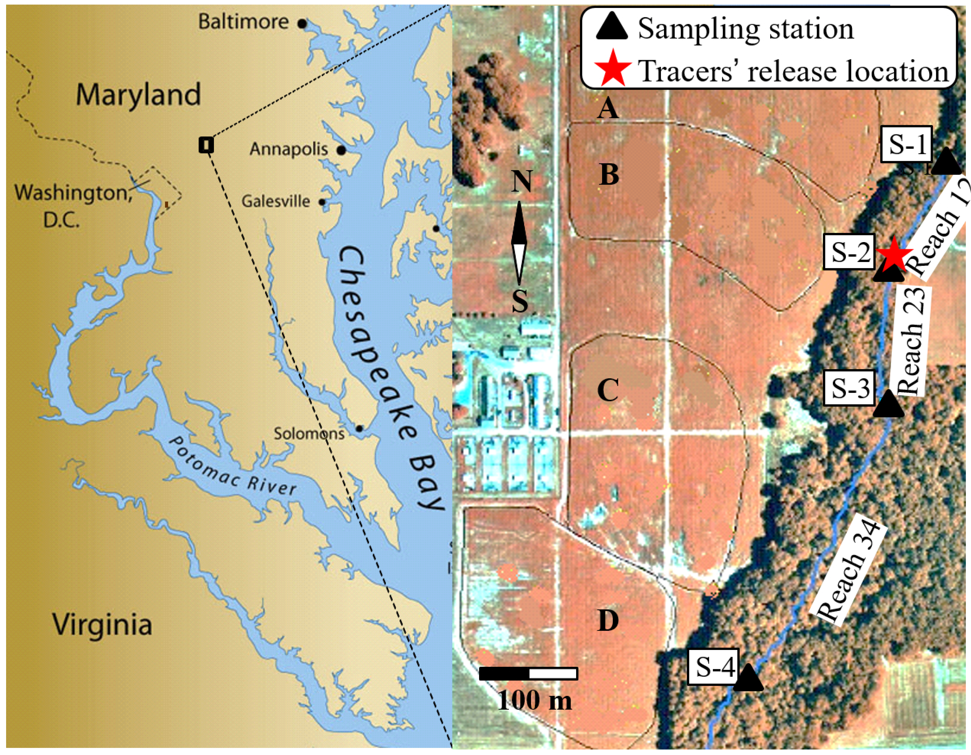
2.1. Description of Study Area

The study site (Figure 1) is located within the Optimizing Production Inputs for Economic and Environmental Enhancement (OPE3) Watershed Research Site of the United States Department of Agriculture (USDA)-Beltsville Agricultural Research Center on the mid-Atlantic coastal plain of Maryland, MD, USA). The entire watershed area is about 70 ha, with 75% employed in agricultural crop production while 15% is under deciduous forest. The site contains a small first-order creek (the Beaver Dam Creek Tributary described in detail by Angier et al., 2005) of ~1100 m length that is instrumented with four stations for monitoring stream flow and water sampling. The creek bed is from 100 to 160 cm wide and the bed slope varies along the creek from 0.0008 to 0.0122 [20] (Cho et al., 2010). The creek runs within a riparian corridor of variable width from about 65 m at its narrowest point, to more than 100 m.

2.2. Sampling Design and Tracer Transport Experiments

Four sampling stations (S-1 to S-4) were instrumented with weirs and automated refrigerated samplers (Sigma 900 Max All Weather Refrigerated Sampler, Hach Company, Loveland, CO, USA) to measure the depth of water and to sample the water in the creek (Figure 1). Stations S-2, S-3 and S-4 are located at a 140, 280 and 630 m distance from S-1, respectively. The weirs have been calibrated to convert the depth of water to flow rate [21]. The sections of the creek between stations S-1 and S-2, S-2 and S-3, and S-3 and S-4 are referred to below as reach 12 (~140 m length), reach 23 (~140 m length), and reach 34 (~350 m length), respectively. The Trimble GeoXM 2005 Series global positioning system was used to determine elevations of the creek bottom at incremental distances along the creek.
Sediment samples were collected one day prior to the tracer injections. Samples were taken from a depth of 1 cm with sterile 50 mL tubes. Sediment sampling began at the last station and continued upstream in approximately 20-m increments until the upper sampling station was reached. Samples were immediately placed on ice and kept in the dark until processing which occurred within 2 h of collection.
Stock solutions of resazurin (Sigma-Aldrich, Spruce Street, St. Louise, MO, USA) and potassium bromide (KBr) (Fisher Scientific, Fair Lawn, NJ, USA) were made in bulk and transported to the field on the morning of the experiment on 20 October 2014. Concentrations of stock solutions were 18 g/L and 10 g/L for Raz and KBr, respectively. Masterflex L/S peristaltic pumps (Model 7535-08, Vernon Hills, Illinois, IL, USA) were used to deliver 2.3 mL/min and 204 mL/min of concentrated Raz and KBr stock solutions, respectively, into a manifold placed 3 m upstream of station S-2 in the stream, which mixed and evenly distributed the tracers horizontally across the stream and injected them over 8 h. Stock solution concentrations and pumping rates were calculated as a function of the average creek discharge measured on the day prior to the experiment such that the concentration at the last station would remain detectable by the analytical techniques available for this experiment. Water samples were collected over 23 h (one sample each hour) at mid-depth in the middle of the stream.

2.3. Microbiological and Chemical Analysis

2.3.1. Bacterial Analysis

Water samples were transported to the laboratory shortly after the 24-h sample was taken at each station. Care was taken to maintain reduced light settings during all parts of sample handling and analysis. E. coli measurements were performed via the membrane filtration method. Approximately 20 mL of sample was vacuum filtered through a 0.45 µm membrane filter which was then placed onto modified mTEC agar (Difco, Sparks, MD, USA). These plates were then incubated at 35 °C for 2 h followed by incubation at 44.5 °C for 22–24 h. Colonies that were red or magenta in color after the incubation period were counted as presumptive E. coli.
Total heterotrophic bacteria were measured by serial diluting water samples into sterile deionized water blanks which were then spread plated onto R2A agar (RemelInc, Lenexa, KS, USA) in 100 µL aliquots. The R2A plates were incubated at room temperature (20–22 °C) and were counted on the 5th and 7th day following plating.
Sediment samples were blended (Model 7011HG, Waring Products Co. Connecticut, CT, USA) on a high blender setting at a ratio of 10 g sediments into 90 mL of sterile D.I. water. The resulting solution was then transferred to sterile beakers which were left to settle for approximately one hour before further processing. The sample solution supernatants were processed in the same manner as detailed above for E. coli and total heterotrophic bacteria.

2.3.2. Smart and Conservative Tracer Analysis

The preparation and measurement of smart tracer concentrations in samples was performed immediately after the microbiological analysis. Samples were shaken thoroughly before having a sub-sample drawn with a sterile 30 mL syringe (BD, Franklin Lakes, NJ, USA). Sub-samples were then passed through a 0.45 µL GF/F glass fiber syringe filter (Pall, Port Washington, New York, NY, USA) into sterile test tubes. Approximately 1.0 mL of each filtered sample was transferred into 1.5 mL scintillation vials and then stored at 4 °C for later conservative tracer analysis. The filtered samples were then transferred into opaque 96-well microplates in a 10:1 ratio of sample to phosphate buffered saline (pH 8) (Calibrochem, San Diego, CA, USA) and mixed thoroughly. Microplates containing the sample and buffer mixture as well as plates containing Raz and Rru standards with the same ratio of buffer addition were wrapped in aluminum foil before being transported to a nearby laboratory for further processing immediately following their completion.
Concentrations of Raz and Rru were measured with a dual monochromator fluorimeter (Spectramax Gemini EM, Molecular Devices, Sunnyvale, CA, USA). The excitation/emission wavelengths for Raz and Rru were set to 630/610 and 586/570, respectively. All samples were measured at 22.5 °C. Calibration was performed by measuring fluorescence at 586 and 630 nm wavelengths in the range of concentration of both compounds from 0.4 to 400 µg/L Concentrations of resazurin C R a z and resorufin C R r u were found using the Marquardt optimization algorithm [22] to minimize the target function,
φ   =   [ F m e a s   ( 586 ) F s i m   ( 586 ) ] 2 + [ F m e a s   ( 630 ) F s i m   ( 630 ) ] 2 ,
where F m e a s   ( 586 ) and F m e a s   ( 630 ) are fluorescence values measured at 586 and 630 nm, respectively,
F s i m   ( 586 )   =   F ( 586 , Raz ) + F ( 586 , Rru ) ,
F s i m   ( 630 )   =   F ( 630 , Raz ) + F ( 630 , Rru ) ,
Values for F(586,Raz), F(586,Rru), F(630,Raz), F(630,Rru) were found by interpolation in calibration data tables that used the “log (concentration)–log fluorescence” for each pair of C R a z and C R r u values used in the search. The optimization algorithm searched for the pair of C R a z and C R r u that would produce a value of the φ smaller than 10−6.
Bromide ion concentration in water samples was measured with the Waters 2695 Separations Module combined with the Waters IC-Pack Anion Column and the Waters 432 Conductivity Detector (Waters Corporation, Milford, MA, USA).

2.4. Flow and Transport Modeling

Most models used to simulate tracer transport in streams assume a constant flow velocity which has been found to be a fitting parameter during the calibration process. In this work’s experiment, flow velocity varied within and between reaches due to groundwater upwelling. Water discharge was measured only at stations S-2 to S-4. Therefore, we applied the Saint-Venant equations to characterize transient water flow in the stream.

2.4.1. Water Flow Governing Equations

The shallow water Saint-Venant equations were used to calculate water depth and discharge. The continuity and the momentum equations, respectively, are [23]:
A t + Q x = q g ,
Q t + x ( Q 2 A + g I 1 ) = g A ( S 0 S F ) + g I 2 + β q g u ,
where A is the cross-sectional area (m2), Q is the discharge (m3 s−1), qg is the groundwater flux to the creek per unit of creek length, (m2 s−1), S F = n 2 u | u | / h 4 / 3 is the friction slope (–), n is the Manning’s roughness coefficient, S0 is the bed slope (–), g = 9.8 is the gravitational acceleration (m s−2), u = Q/A is the average flow velocity (m s−1), β 1 accounts for the effect of groundwater upwelling on momentum of flow, x is the distance along creek (m), and t is time (s),
I 1 = 0 h ( h z ) w ( x , z ) d z   and   I 2 = 0 h ( h z ) w ( x , z ) x d z ,
where h is height of water column (m) and w is the creek width (m).
For simplicity, we considered a stream with a rectangular cross-section of the width W(x), then
I 1 = A h / 2 ,   I 2 = b h 2 / 2 ,
where b = W / x .

2.4.2. Transport Governing Equations
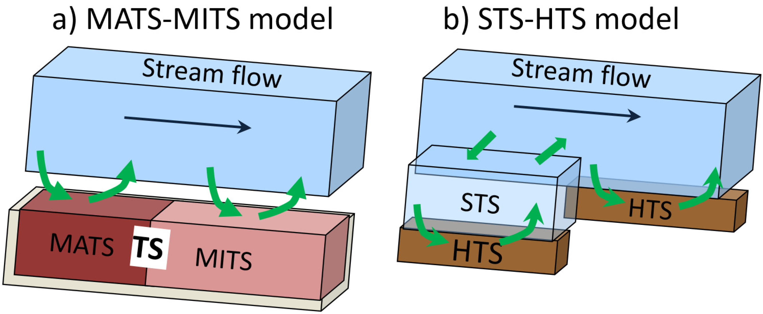
The advection–dispersion equation was applied to simulate the transport of a conservative Br tracer and Raz–Rru tracers during an experiment in the Beaver Dam Creek Tributary. The 1D stream solute transport model accounts for advection–dispersion, lateral inflow–outflow, exchange with TS, and linear decay–transformation–production reactions. Two mathematical models are considered. Figure 2 shows their conceptual representation.
MATS–MITS, adopted from [15] and modified for transient flow conditions, accounts for two compartments in TS, namely, the metabolically active (MATS) and metabolically inactive (MITS) compartments. The main stream water was considered as metabolically inactive. The STS–HTS model (current research) considers the interaction of tracers experiencing advective transport in a stream with STS (dead zones represented by stagnant pools, eddies etc.) and metabolically active stream bed sediments representing hyporheic transient storage (HTS). Stream bed concentration components were considered separately for both the main stream and STS.

MATS–MITS Model

For the conservative tracer transport, the governing equations in the stream and TS [5], respectively, are
( A C ) t = x ( A D C x ) ( Q C ) x α s A ( C S ) + q g + C g q g C ,
( A s S ) t = α s A ( C S ) ,
where C and S are concentrations in the stream and TS, respectively (ML−3); D is the dispersion coefficient (L2T−1); α s are the stream–TS exchange rate coefficients (T−1), respectively; Cg is the tracer concentration in the groundwater (ML−3); and q g ± = ( q g ± | q g | ) / 2 .
For reactive tracers, such as Raz and Rru, decay and transformation in both MITS and MATS are taken into account with
( A C 1 ) t = x ( A D C 1 x ) ( Q C 1 ) x α s A [ C 1 f a S 1 a ( 1 f a ) S 1 i ] + q g + C 1 g q g C 1 ( k w 1 l + k w 12 l ) A C 1 ,
( A C 2 ) t = x ( A D C 2 x ) ( Q C 2 ) x α s A [ C 2 f a S 2 a ( 1 f a ) S 2 i ] + q g + C 2 g q g C 2 k w 2 l A C 2 + k w 12 l A y C 1 ,
( A s S 1 l ) t = α s A ( C 1 S 1 l ) ( k w 1 l + k w 12 l ) A s S 1 l ,
( A s S 2 l ) t = α s A ( C 2 S 2 l ) k w 2 l A s S 2 l + k w 12 l A s y S 2 l ,
where subscripts 1 and 2 refer to Raz and Rru, respectively, in Equations (12) and (13); l = a and i correspond to MATS and MITS, respectively; fa represents the MATS fraction; k w 1 l , k w 12 l and k w 2 l are rates of Raz decay, Raz to Rru transformation, and Rru decay in MATS (l = a) and MITS (l = i), respectively; and y = MRru/MRaz is the conversion factor [12].

STS–HTS Model

The governing equation of conservative tracer transport in a stream that considers STS and HTS compartments, respectively, are
( A C ) t = x ( A D C x ) ( Q C ) x α s A ( C S ) α b A ( C C b ) + q g + C g q g C ,
( A s S ) t = α s A ( C S ) + α b A s (   S C b s ) ,
h b θ C b t = α b h ( C C b ) ,
h b θ C b s t = α b h ( S C b s ) ,
where Cb and Cbs are the tracer concentrations in bed sediments (HTS) related to the stream and STS, respectively (ML−3); α b is the stream–STS and the stream–stream bed exchange rate coefficients (T−1); and h b and θ are the thickness and the porosity of a sediment layer (HTS) storing the tracer.
The governing equations for Raz and Rru transport in a stream that considers STS and HTS compartments, respectively, are
( A C 1 ) t = x ( A D C 1 x ) ( Q C 1 ) x α s A ( C 1 S 1 ) α b A ( C 1 C 1 b ) + q g + C 1 g q g C 1 ( k w 1 i + k w 12 i ) A C 1 ,
( A C 2 ) t = x ( A D C 2 x ) ( Q C 2 ) x α s A ( C 2 S 2 ) α b A ( C 2 C 2 b ) + q g + C 2 g q g C 2 k w 2 i A C 2 + k w 12 i A C 1 ,
( A s S 1 ) t = α s A ( C 1 S 1 ) + α b A s ( S 1 C 1 b s ) ( k w 1 i + k w 12 i ) A S 1 ,
( A s S 2 ) t = α s A ( C 2 S 2 ) + α b A s ( S 2 C 2 b s ) k w 2 i A S 2 + k w 12 i A S 2 ,
h b θ R 1 C 1 b t = α b h ( C 1 C 1 b ) ( k b 1 + k b 12 ) h b C 1 b ,
h b θ R 2 C 2 b t = α b h ( C 2 C 2 b ) k b 2 h b C 1 b + k b 12 h b C 1 b ,
h b θ R 1 C 1 b s t = α b h ( S 1 C 1 b s ) ( k b 1 + k b 12 ) h b C 1 b s ,
h b θ R 2 C 2 b s t = α b h ( S 2 C 2 b s ) k b 2 h b C 1 b s + k b 12 h b C 1 b s ,
where k w 1 i , k w 12 i , and k w 2 i are the rates of Raz decay, Raz to Rru transformation, and Rru decay (T−1) in the stream and TS, respectively; k b 1 , k b 12 , k b 2 and are the rates of Raz decay, Raz to Rru transformation, and Rru decay (T−1) in the stream bed, respectively; R i = 1 + ρ b K D i / θ is the retardation facto; ρ b is the sediment bulk density (ML−3); and K D i is the linear sorption partitioning coefficient (L3/M).
We assumed that the storage ratio parameter, fs = As/A, does not change with time, but it is reach specific. Longitudinal dispersion is expected to increase with increasing discharge and flow velocity [24], due to turbulence structures developing within the water column. Therefore, we adopted a linear dependence of the dispersion coefficient on the flow velocity [25], i.e., D = aLu, where aL is the dispersivity (L).

2.4.3. Initial and Boundary Conditions, Numerical Solution

For the Saint-Venant equations, the initial conditions define the distribution of water fluxes and water depth along the creek at t = 0; while boundary conditions specify the value of the flux as a function of time at the stream inlet (when supercritical flow is considered, the value of the water depth is also prescribed), and the transmissive boundary at the outlet. For the transport equation, the initial conditions define the concentrations of tracer in the water and bed layer along the creek at t = 0, while boundary conditions specify the value of concentrations in the water column as a function of time at the stream inlet, and the zero-dispersive flux (Neumann boundary condition) at the outlet. The inlet boundary was assigned at station S-2, and the outlet boundary was 4 m downstream of station S-4.
The Saint-Venant equations were solved numerically by the finite volume method using a central-upwind scheme [26], the fourth order Runge-Kutta method with the estimate of truncation error [27], and adaptive time step-size control [22]. The transport equations were solved by using an implicit finite differences method and applying the front limitation algorithm [28]. The space step was 10 m, while the time step varied to fit both stability criteria to solve the Saint-Venant equation and to keep the Courant number to be less than 0.5 for the transport equation solution. The FORTRAN code was developed to implement the numerical algorithms. Benchmarking was performed using the dam break solution [29] for the Saint-Venant equations, and analytical solutions for the advection–dispersion equation [30].

2.5. Model Calibration

Analysis of the Beaver Dam Creek experimental data relied on solving the inverse problem using a least squares optimization and PEST code [31]. The objective function, used for model calibration, was the weighted sum of squared residuals between observed and simulated concentrations. The unit weights were prescribed for all concentrations. Reach-specific model parameters were estimated using the measured concentrations of Br, Raz and Rru at stations S-3 and S-4.
The first step in calibration was to estimate transport parameters for each model: dispersivity (aL), TS ratio (fs) and exchange rate between the stream and the TS ( α s ) for each reach using Br breakthrough curves. For the STS–HTS model, an additional parameter of exchange rate between the stream and the stream bed ( α b ) was determined. Calibration started from reach 23 by searching the above parameters for this reach, while holding values (based on an initial guess) of these parameters at the downstream reach (34) constant. When satisfactory agreement between observed and simulated breakthrough curves (BTCs) at station S-3 was achieved, the calibration procedure was performed for reach 34, accepting the parameters found for reach 23 as constant.
The second step in the calibration was estimating the parameters of the reactive tracers Raz and Rru. We used the values of the dispersivity found by calibrating the transport model for Br. For the MATS–MITS model, we searched for the values of the following parameters: the TS ratio (fs), the exchange rate between the stream and TS ( α s ), the MATS ratio (fa), and the MATS decay and transformation rate coefficients ( k w 1 a , k w 12 a and k w 2 a ). For the STS–HTS model, the calibration was performed with respect to the TS ratio (fs), exchange rate between the stream and TS, ( α s ), the exchange rate between the stream and stream bed ( α b ), and the stream-bed decay and transformation rate coefficients ( k b 1 , k b 12 and k b 2 ). The MITS and the STS decay and transformation rate coefficient values for the stream were adopted from [12] where k w 1 i = 8.03 × 10⁻¹¹ s−1, k w 12 i = 2.75 × 10⁻⁷ s−1 and k w 2 i = 4.86 × 10⁻⁷ s−1, respectively. These same values were used by Argerich et al. [15] to simulate Raz and Rru transport in a steep, second-order stream located in the western Cascade Mountains of Oregon. The thickness of the bed sediment layer, hb, representing the HTS in the STS–HTS model was set to 0.01 m. [32], because most of the microorganisms were found in this layer, and the estimated penetration of the tracer diffusion front into the HTS during the experiment did not exceed 0.01 m. Note that Knapp et al. [33] concluded that the benthic biolayer was found to be on average 2 cm thick, ranging from one third to one half of the full depth of the hyporheic zone.
Two sets of calibrations were performed with the STS–HTS model. In the first calibration (Cal-1), the above-mentioned values of the decay and transformation rate coefficients in the stream and STS were used. In the second calibration (Cal-2), the values of the decay and transformation rate coefficients in the stream and STS were found by calibration. It was not possible to find these parameters for the MATS–MITS model in MITS by solving an inverse solution because the mathematical formulation of the mass balance in the MITS and MATS zones are identical.
The reactive tracers have been shown to undergo sorption to the bed sediments [15,34]. The parameters of the sorption of Raz and Rru isotherms for the sediments in the studied creek are unknown, therefore, we assumed that irreversible sorption was taken into account by the decay rate coefficients of these tracers in MATS [15] and in the stream bed.
The corrected Akaike information criterion [35] was used to discriminate between the models
A I C c = 2 p + N [ ln ( R S S N ) ] + 2 p ( p + 1 ) N p 1 ,
where RSS is the residual sum of squares and p is the number of parameters. The Akaike statistic values were computed for each stream reach and the model used for simulations. The preferred model was the model with the lowest AICc value. The AICc not only rewards suitability of fit, but also includes a penalty that is an increasing function of the number of estimated parameters. This penalty discourages overfitting.

3. Results and Discussion

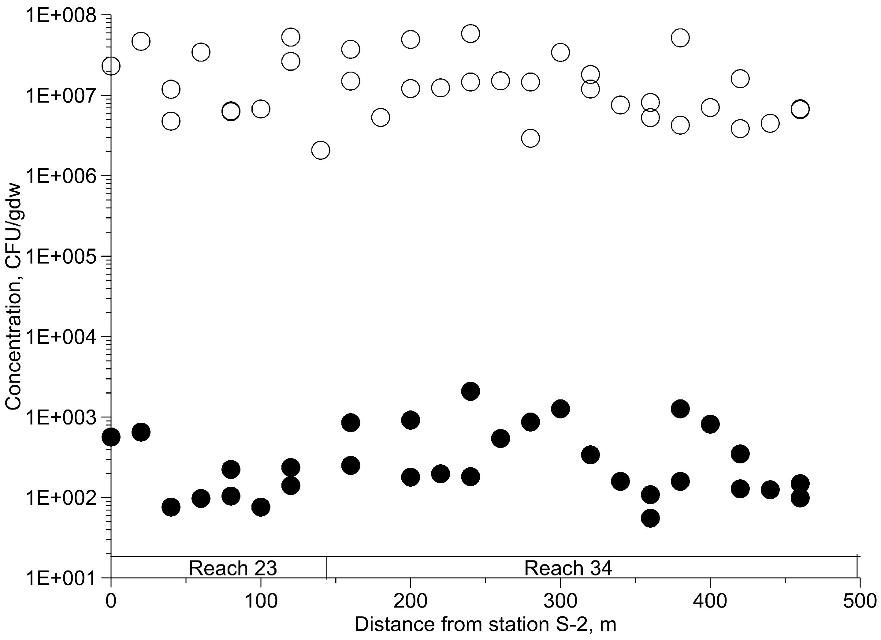
3.1. Sediment Composition

Reaches 23 and 34 had clay percentages of 18.0 ± 2.1 and 17.7 ± 3.0, sand percentages of 50.4 ± 9.2 and 69.6 ± 5.9, and silt percentages of 31.2 ± 7.6 and 12.7 ± 3.7, respectively, in their textural composition. Reach 34 had markedly lower silt content as compared with Reach 23. The difference between the average clay contents in the two reaches was not significant. Variations in sediment particle size along the creek are at least partially attributable to the channel slope of the creek [20]. The relative contents of silt were greatest in sites where the channel slope was the lowest.
The concentrations of E. coli and total heterotroph bacteria in the sediment along the creek are shown in Figure 3. The results illustrate that the E. coli concentrations are a few orders of magnitude smaller than the concentration of total heterotrophs and both can vary substantially within relatively short distances. The average concentration of E. coli in reach 34 was twice of that in reach 23, while the average concentration of total heterotrophs was 1.3 times higher in reach 23 compared with the reach 34. These differences may be related to the differences in association of E. coli with particles of different sizes. Such associations have been shown to be stronger with silt and clay than with sand particles [36,37]. Garzio-Hadzik et al. [38] observed an increase in sediment E. coli concentrations with increasing silt content in the sediment of the creek where our experiments were conducted.

3.2. Stream Flow

The measured water discharge during the study at S-2, S-3 and S-4 in the creek varied from 70–97 mL/s, 527–595 mL/s and 853–959 mL/s, respectively. The groundwater upwelling flux into the creek was calculated for each section of the creek between the weirs based on the water balance as a difference between the average discharge at the reach outlet and inlet per unit length. The calculated mean values of groundwater upwelling flux for reaches 23 and 34 were 3.32 × 10⁻⁴ and 1.01 × 10⁻⁴ m2/s, respectively. The bed roughness parameter (n) for each reach was adopted from [32] as an average of values obtained during the previous calibrations of the flow model, namely, n = 0.12 and 0.09 for reaches 23 and 34, respectively. The measured water discharge at S-2 was accepted as the upstream boundary condition. The simulated water discharge at stations S-3 and S-4 corresponded well to measured discharge at these locations. In reaches 23 and 34, simulated flow velocity varied in a range of 0.022–0.036 m/s and 0.027–0.049 m/s, respectively.

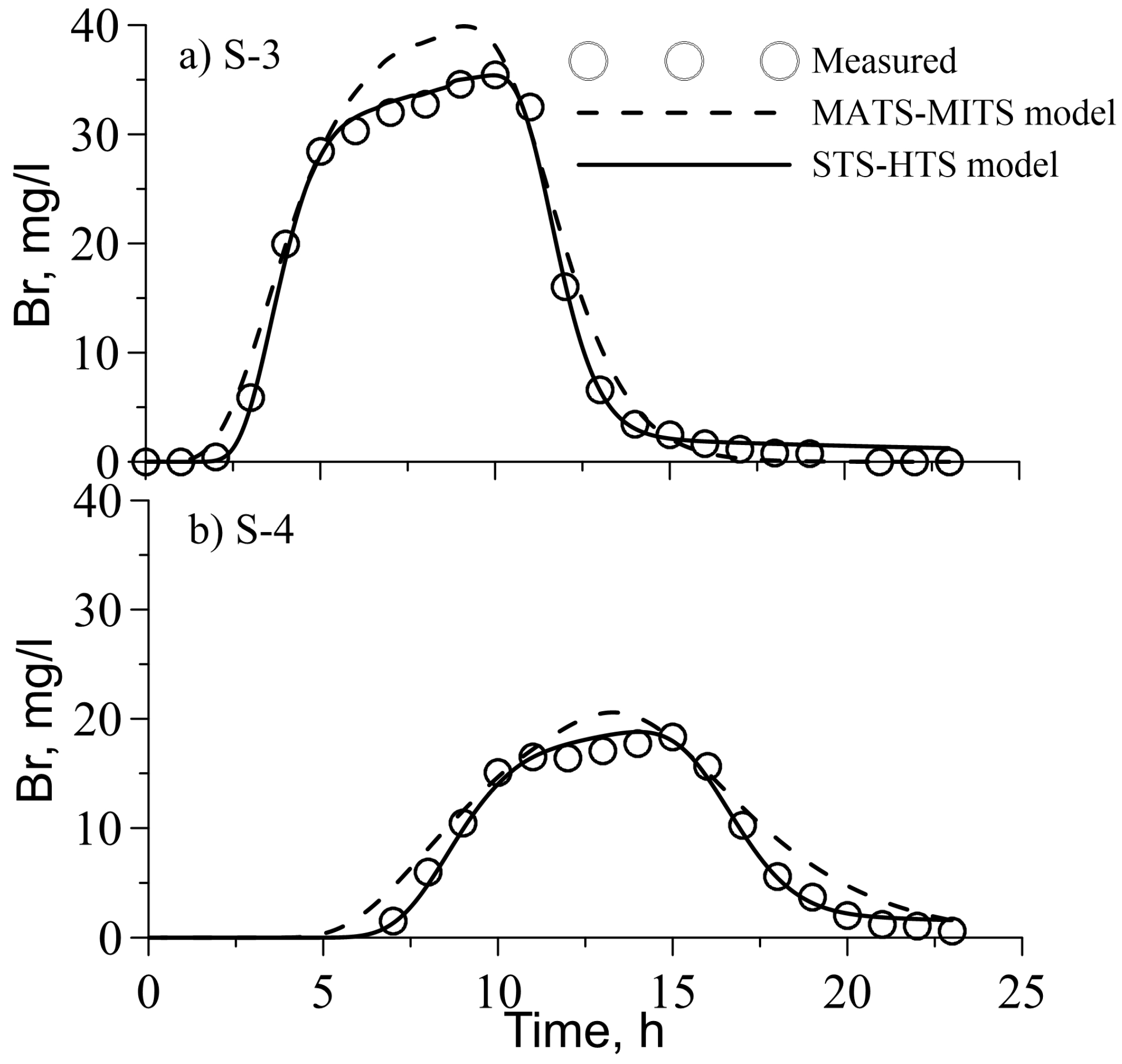
3.3. Conservative Tracer (Br) Transport

Figure 4 presents a comparison between the observed and simulated BTCs of the Br tracer for two models. The observed BTCs are skewed and exhibit long tails which means that the TS is an important mixing mechanism. The agreement between the observed and simulated BTCs of Br is better for the STS–HTS model compared to the MATS–MITS model, as has been indicated by the AICc criterion and standard errors (Table 1). The values of the estimated transport parameters are shown in Table 1. The dispersivity values (aL) for both the models are the same order of magnitude. For the MATS–MITS model, the dispersivity is similar in reach 23 and smaller in reach 34 compared to the STS–HTS model. These dispersivities provide dispersion coefficients in a range of 0.044–0.234 m2/s, which is consistent with the values provided by many reports [5,6,9,39].
The estimated values of the TS ratio (fs = As/A, Table 1) are larger for the MATS–MITS model compared to the STS–HTS model because the latter accounts for the tracer retention in HTS, in addition to STS. The fs magnitude is also around three times larger for reach 23 compared to reach 34 and is attributed to the fact that water flux in reach 23 was substantially smaller than the water flux in the downstream reach.
The TS exchange rate parameter, α s , estimated for the MATS–MITS model is about an order of magnitude smaller than α s representing the exchange with the STS for the STS–HTS model, while the exchange rate, α b , of the stream–HTS is two orders of magnitude smaller than α s for the STS–HTS model (Table 1). Thus, the range for the TS in the MATS–MITS model is somewhere between α s and α b for the STS and HTS, respectively. It should be noted that both exchange rates are smaller in the downstream reach compared to the upstream one.
Table 2 presents the measured Br mass recovery and the estimated recovery with the two models at station S-4. The STS–HTS model overestimates the measured mass recovery by around 7%, while the MATS–MITS model predicts almost full Br mass recovery. When the experiment ended, the simulations with the STS–HTS model indicated that 12% of the Br mass remained stored in the stream bed sediments, this is attributed to the small exchange rate between the main stream and the HTS. In contrast, when the experiment ended, the MATS–MITS model predicted almost complete Br flushing from the stream and TS. This difference helps explain why the fit of the observed bromide BTCs with the MATS–MITS model is less accurate than the BTCs estimated with the STS–HTS model. For reach 23, the calibration of the MATS–MITS model led to increased dispersivity values and extended tails in simulated BTC in an attempt to reduce the differences between maximum observed and simulated concentrations (Figure 4).

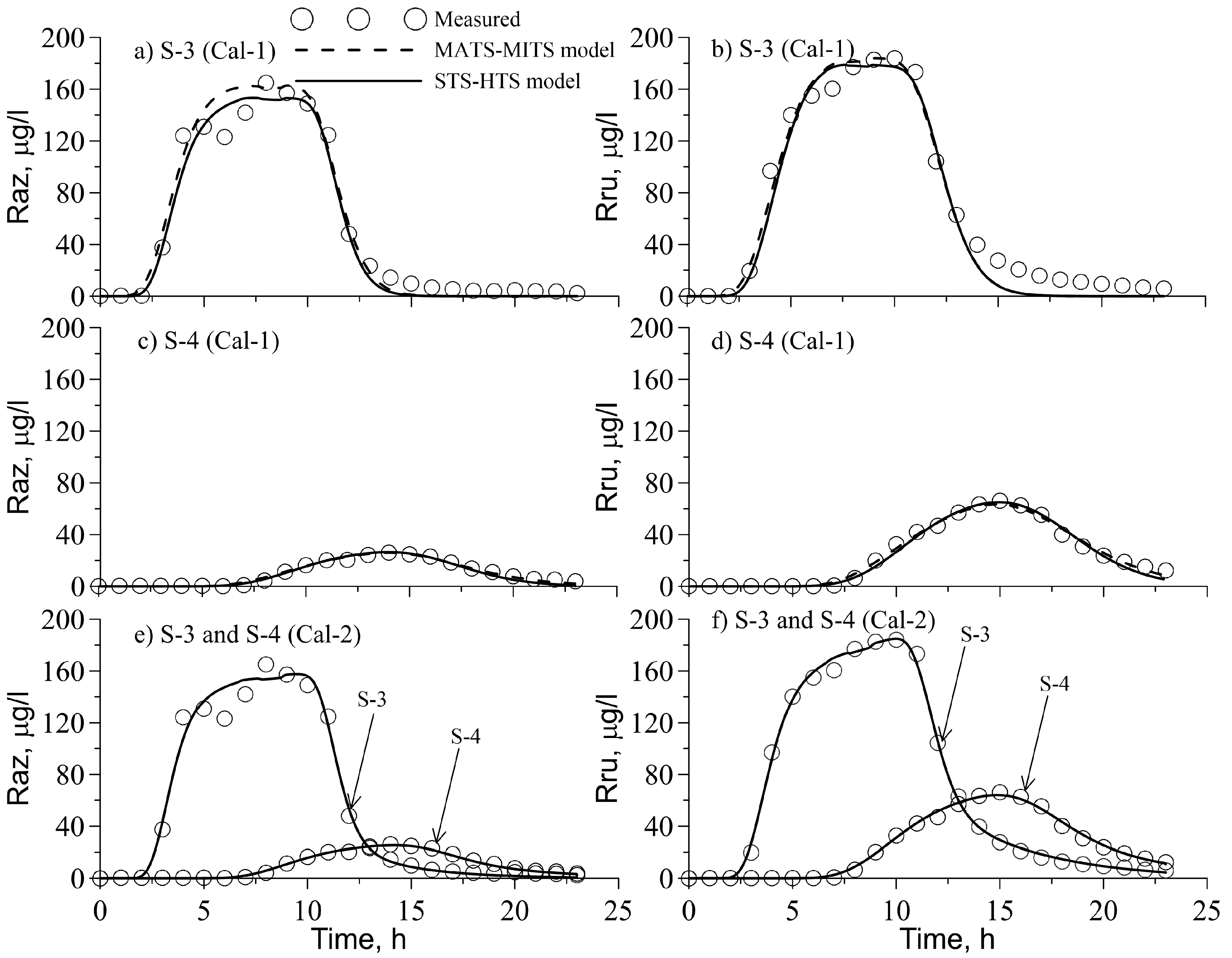
3.4. “Smart” Tracer Raz-Rru Transport

Figure 5 shows the observed and simulated Raz–Rru concentrations at the two creek stations. Simulation results with the MATS–MITS model and the STS–HTS model were quite similar (Figure 5a–d) when the decay and transformation rates in the stream and STS were set to values found in [12]. Both models performed well in fitting the observed BTC Raz and Rru tracers. An exception occurred in the tailing part of the BTC at S-3 approximately 13 h after the experiment started where the simulated concentrations were significantly lower than the observed concentrations. The magnitude of the AICc and standard error (Table 3) evaluation parameters indicated that the MATS–MITS model fit the experimental data slightly better compared to the STS–HTS model. An attempt to calibrate the MATS–MITS model with the parameters of TS ratio (fs) and stream–TS exchange rate ( α s ) obtained in the Br simulations was not successful and the agreement between the observed and simulated concentrations was much worse when compared to the BTCs presented in Figure 5.
A similar model behavioral pattern was observed for the STS–HTS model with respect to the stream–HTS exchange rate ( α b ). It was assumed that the reactive tracers undergo sorption on woody debris, plants and other organic surfaces located in the main stream and, therefore, the TS can delay breakthrough of these solutes when compared to Br. The exchange rate between the main stream and HTS can be faster for the smart tracers compared to Br because the latter is subject to negative sorption on sediments. Table 3 presents the model parameters found by calibration. The TS ratio, fs, for the Raz-Rru tracers was around 4% and 6% larger in Reach 23 compared with that found for Br, while for Reach 34 during the first simulation these differences were 89% and 55% for the MATS–MITS model and the STS–HTS model, respectively. For the MATS–MITS model, the exchange rates α s for Raz-Rru were approximately 6.3 and 2.2 times the exchange rates for Br in Reaches 23 and 34, respectively. For the STS–HTS model, the exchange rate of the stream–HTS, α b , was more that an order of magnitude larger for the reactive tracer compared to the conservative tracer. The estimated decay and transformation rate coefficients for MATS and HTS have generally small values (Table 3). Their magnitudes are similar to those parameters (k1 = 6.1 × 10⁻⁵, k12 = 22.5 × 10⁻⁵, and k2 = 44.4 × 10⁻⁵ s−1) obtained in [12] for MATS in a forested second-order stream in Riera de Santa Fe del Montseny (Catalonia, NE Spain). These values were also similar to a range of values (0.02–62.2) × 10−5 s−1 assessed by Lemke et al. [34] in laboratory column experiments on Raz and Rru transport, sorption, and transformation under neutral and alkaline conditions using two types of streambed sediments. The exceptions to these estimated values were large Raz decay rates in Reach 23 and Raz to Rru transformation rates in Reach 34 ( k w 1 a = 248 × 10−5 s−1, k w 12 a = 293 × 10−5 s−1) in the MATS for the MATS-MITS model.
The second calibration of the STS–HTS model when the decay and transformation parameters were freely optimized in all the compartments (i.e., main stream, STS, and HTS) provided better fits compared to the MATS–MITS model and the STS–HTS model during the first calibration. The BTC tails of both Raz and Rru were described fairly well by the model (Figure 5e,f). The AICc criterion and standard errors also indicated that in this case the STS–HTS model performed better compared to the MATS–MITS model and the STS–HTS model with fixed parameters during the first calibration, despite the large number of parameters (eight) that were simultaneously optimized for each reach. However, in this case there is likely to be a problem of parameter equifinality, and additional information is required to avoid it, such as, e.g., cross-sectional stream velocity distributions [9] or calculated temporal moments and uptake length [15]. The TS ratio (fs) determined in the second calibration was slightly smaller and larger in Reaches 23 and 34, respectively, compared to same parameters obtained during the first calibration. The stream–HTS exchange rate ( α b ) during the second calibration was 1.5% and 3.8% of the values of this parameter obtained during the first calibration for Reaches 23 and 34, respectively. The most striking feature of the simulations was that the values of Raz and Rru decay rates in the stream and STS were orders of magnitude higher when compared to the decay rates reported in [12]. These higher values for the decay rate were used during the first calibration and with the MATS–MITS model. It is speculated that these higher values could be due to Raz and Rru sorption on plant woods and other organic surfaces in the stream. The very high transformation rates of Raz to Rru conversion in the stream and STS indicated that a considerable proportion of the Raz transformations may occur in these compartments. This transformation may be attributed to a relatively high concentration of total heterotrophs in the stream water, varying in range from 2.3 × 10⁴ to 1.3 × 10⁶ CFU/mL. The Raz decay rates in the HTS were considerably smaller during the second calibration compared with the first calibration (Table 3), which indicated a large degree of uncertainty in determining those parameters.
Table 2 demonstrates the components of the mass balance for Raz and Rru. The simulated Raz and Rru mass recovery at S-4 were 3.8–3.9% and 9.5–9.9% of injected Raz mass, respectively, which was close to the measured 3.9% and 9.8% mass recovery for these tracers. Simulations indicated that approximately 95% of the Raz mass decayed and was transformed to Rru. The estimated mass of the Rru decay was similar in all simulations (13.1–13.7% of injected Raz), as well as the total Rru mass production (24.4–25.2% of injected Raz). The MATS–MITS model and the STS–HTS model during the first calibration predicted that more than 90% of Rru production occurred in the MATS or HTS. During the second calibration with the STS–HTS model, Rru production in the stream was 2.8 times greater than in the HTS. These discrepancies may be partially attributable to the transformation rate not being independently determined in the study, but rather being found by inverse solutions that possibly also account for irreversible sorption. Thus, “the effects of sorption might misleadingly be captured by parameters that address other processes in standard modeling approaches, resulting in an erroneous characterization of hyporheic exchange and microbial activity in the hyporheic zone” [34].

4. Conclusions

In this study, a numerical model of transient water flow and the transportation of Br and Raz-Rru tracers in streams was developed that accounts for the exchange with the STS and HTS (the STS–HTS model). The model was used to simulate a tracer experiment by injecting conservative (Br) and reactive (Raz) tracers into the perennial first-order Beaver Dam Creek Tributary in a riparian zone within Maryland, MD, USA. The modeling results were compared with simulations by conceptually different models that considered TS as being composed of MATS and MITS compartments (the MATS–MITS model). Both models reproduce the experimental data reasonably well. The STS–HTS model more accurately fits the observed Br concentrations because different rates of exchange were considered between the stream and STS, and the stream and HTS, unlike the MATS–MITS model that used a single exchange rate coefficient. Both models displayed similar results in simulating Raz and Rru tracer migration when the values of the decay and transformation rates of these tracers in the main stream, MITS and STS were adopted from literature. The BTCs simulated using these models were not well-fitted in the tail portion of the BTCs for either model. The values of the adopted coefficients were very small, thus most of the decay and transformation processes within the creek’s upstream reach zones occurred in the MATS compartment for the MATS–MITS model and in the HTS compartment for the STS–HTS model. Therefore, the effects of different exchange rates for the stream–STS and stream–HTS were diminished for the conservative tracer, when compared.
The simulations with the STS–HTS model when the reaction parameters were searched for all model compartments provided good fits for the entire observed BTCs, however, the results of the Raz to Rru transformation remained uncertain due to problems of parameter equifinality.

Acknowledgments

This research was partially supported by the ARS-USDA via Specific Cooperative Agreement with the University of Maryland, College Park on the project # 8042-12630-008-24 “Using Modeling to Develop Monitoring Strategy and Scheduling for Microbial Quality of Irrigation Water Sources”.

Author Contributions

Alexander Yakirevich developed the numerical model, carried out simulations and participated in writing the manuscript. Daniel Shelton provided microbiological support in the planning of the experiment and critically evaluated the manuscript. Robert Hill critically evaluated the manuscript and provided support to coauthors in the writing process. Lynda Kiefer, Matthew Stocker, and Ryan Blaustein performed the experiment, helped analyze the data, and aided in the writing process. Michael Kuznetsov aided in developing the numerical model. Greg McCarty provided equipment necessary for the study and helped perform the experiment. Yakov Pachepsky designed the experiment and participated in data analysis and manuscript writing.

Conflicts of Interest

The authors declare no conflict of interest.

References

  1. Vörösmarty, C.J.; McIntyre, P.B.; Gessner, M.O.; Dudgeon, D.; Prusevich, A.; Green, P.; Glidden, S.; Bunn, S.E.; Sullivan, C.A.; Liermann, C.R.; et al. Global threats to human water security and river biodiversity. Nature 2010, 467, 555–561. [Google Scholar]
  2. Boano, F.; Harvey, J.W.; Marion, A.; Packman, A.I.; Revelli, R.; Ridolfi, L.; Wörman, A. Hyporheic flow and transport processes: Mechanisms, models and biogeochemical implications. Rev. Geophys. 2014, 52, 603–679. [Google Scholar] [CrossRef]
  3. US EPA, National Summary of State Information. Assessed Waters of United States. 2017. Available online: https://ofmpub.epa.gov/waters10/attains_nation_cy.control (accessed on 24 June 2017).
  4. Zaramella, M.; Bottacin-Busolin, A.; Tregnaghi, M.; Marion, A. Exchange of pollutants between rivers and the surrounding environment: Physical processes, modelling approaches and experimental methods. In Rivers-Physical, Fluvial and Environmental Processes; Rowinski, P., Radecki-Pawlik, A., Eds.; Springer International Publishing: Basel, Switzerland, 2015; pp. 567–590. [Google Scholar]
  5. Bencala, K.E.; Walters, R.A. Simulation of solute transport in a mountain pool-and-riffle stream: A transient storage model. Water Resour. Res. 1983, 19, 718–724. [Google Scholar] [CrossRef]
  6. Harvey, J.W.; Wagner, B.J.; Bencala, K.E. Evaluating the reliability of the stream tracer approach to characterize stream-subsurface water exchange. Water Resour. Res. 1996, 32, 2441–2451. [Google Scholar] [CrossRef]
  7. Runkel, R.L. One-Dimensional Transport with Inflow and Storage (OTIS): A Solute Transport Model for Streams and Rivers: U.S. Geological Survey, Water-Resources Investigations Report 98-4018; U.S. Geological Survey: Denver, CO, USA, 1998; Volume 73.
  8. Gooseff, M.N.; Bencala, K.E.; Wondzell, S.M. Solute transport along stream and river networks. In River Confluences, Tributaries and the Fluvial Network; Rice, S.P., Roy, A.G., Rhoads, B.L., Eds.; John Wiley & Sons, Ltd.: Chichester, UK, 2008; pp. 395–417. [Google Scholar]
  9. Briggs, M.A.; Gooseff, M.N.; Arp, C.D.; Baker, M.A. A method for estimating surface transient storage parameters for streams with concurrent hyporheic storage. Water Resour. Res. 2009, 45. [Google Scholar] [CrossRef]
  10. Runkel, R.L. A new metric for determining the importance of transient storage. J. N. Am. Benthol. Soc. 2002, 21, 529–543. [Google Scholar] [CrossRef]
  11. Haggerty, R.; Argerich, A.; Martí, E. Development of a “smart” tracer for the assessment of microbiological activity and sediment-water interaction in natural waters: The resazurin-resorufin system. Water Resour. Res. 2008, 44, W00D01. [Google Scholar] [CrossRef]
  12. Haggerty, R.; Martí, E.; Argerich, A.; von Schiller, D.; Grimm, N. Resazurin as a “smart” tracer for quantifying metabolically active transient storage in stream ecosystems. J. Geophys. Res. 2009, 114, G03014. [Google Scholar] [CrossRef]
  13. González-Pinzón, R.; Haggerty, R.; Myrold, D.D. Measuring aerobic respiration in stream ecosystems using the resazurin-resorufin system. J. Geophys. Res. 2012, 117, G00N06. [Google Scholar] [CrossRef]
  14. González-Pinzón, R.; Haggerty, R.; Argerich, A. Quantifying spatial differences in metabolism in headwater streams. Freshwater Sci. 2014, 33, 798–811. [Google Scholar] [CrossRef]
  15. Argerich, A.; Haggerty, R.; Martí, E.; Sabater, F.; Zarnetske, J. Quantification of metabolically active transient storage (MATS) in two reaches with contrasting transient storage and ecosystem respiration. J. Geophys. Res. 2011, 116, G03034. [Google Scholar] [CrossRef]
  16. Kerr, P.C.; Gooseff, M.N.; Bolster, D. The significance of model structure in one-dimensional stream solute transport models with multiple transient storage zones-competing vs. nested arrangements. J. Hydrol. 2013, 497, 133–144. [Google Scholar] [CrossRef]
  17. Gooseff, M.N.; McKnight, D.M.; Runkel, R.L.; Duff, J.H. Denitrification and hydrologic transient storage in a glacial meltwater stream, McMurdo Dry Valley, Antarctica. Limnol. Oceanogr. 2004, 49, 1884–1895. [Google Scholar] [CrossRef]
  18. Harvey, J.W.; Saiers, J.E.; Newlin, J.T. Solute transport and storage mechanisms in wetlands of the Everglades, south Florida. Water Resour. Res. 2005, 41, W05009. [Google Scholar] [CrossRef]
  19. Choi, J.; Harvey, J.W.; Conklin, M.H. Characterizing multiple timescales of stream and storage zone interaction that affect solute fate and transport in streams. Water Resour. Res. 2000, 36, 1511–1518. [Google Scholar] [CrossRef]
  20. Cho, K.H.; Pachepsky, Y.A.; Kim, J.H.; Guber, A.K.; Shelton, D.R.; Rowland, R. Release of Escherichia coli from the bottom sediment in a first-order creek: Experiment and reach-specific modeling. J. Hydrol. 2010, 391, 322–332. [Google Scholar] [CrossRef]
  21. Hively, W.D.; McCarty, G.W.; Angier, J.T.; Geohring, L.D. Weir design and calibration for stream monitoring in a riparian wetland. Hydrol. Sci. Technol. 2006, 22, 71–82. [Google Scholar]
  22. Press, W.W.; Teukolsky, S.A.; Vetterling, W.T.; Flannery, B.P. Numerical Recipes in Fortran: The Art of Scientific Computing, 2nd ed.; Cambridge University Press: New York, NY, USA, 1992. [Google Scholar]
  23. Cunge, J.; Holly, F.; Verwey, A. Practical Aspects of Computational River Hydraulics; Pitman Publisher Ltd.: London, UK, 1980. [Google Scholar]
  24. Wallis, S.G.; Manson, J.R. Methods for predicting dispersion coefficients in rivers. Water Manag. 2004, 157, 131–141. [Google Scholar] [CrossRef]
  25. Foppen, J.W.; Seopa, J.; Bakobie, N.; Bogaard, T. Development of a methodology for the application of synthetic DNA in stream tracer injection experiments. Water Resour. Res. 2013, 49, 5369–5380. [Google Scholar] [CrossRef]
  26. Kurganov, A.; Petrova, G. A central-upwind scheme for nonlinear water waves generated by submarine landslides. In Hyperbolic Problems: Theory, Numerics, Applications; Benzoni-Gavage, S., Serre, D., Eds.; Springer: Heidelberg, Germany, 2008; pp. 635–642. [Google Scholar]
  27. England, R. Error estimates for Runge-Kutta type solutions to systems of ordinary differential equations. Comput. J. 1969, 12, 166–170. [Google Scholar] [CrossRef]
  28. Haefner, F.; Boy, S.; Wagner, S.; Behr, A.; Piskarev, V.; Palatnik, V. The ‘front limitation’ algorithm. A new and fast finite-difference method for groundwater pollution problems. J. Contam. Hydrol. 1997, 27, 43–61. [Google Scholar] [CrossRef]
  29. Stoker, J.J. Water Waves. The Mathematical Theory with Applications; Interscience Publishers Inc.: New York, NY, USA, 1957; Volume 609. [Google Scholar]
  30. van Genuchten, M.T.; Alves, W.J. Analytical Solutions of the One-Dimensional Convective-Dispersive Solute Transport Equation. USDA ARS Technical Bulletin N° 1661; U.S. Salinity Laboratory: Riverside, CA, USA, 1982.
  31. Doherty, J. PEST, Model-Independent Parameter Estimation, User’s Manual, 5th ed.; Watermark Numerical Computing: Brisbane, Australia, 2004. [Google Scholar]
  32. Yakirevich, A.; Pachepsky, Y.A.; Gish, T.J.; Guber, A.K.; Shelton, D.R.; Cho, K.H. Modeling transport of Escherichia coli in a creek during and after artificial high-flow events: Three year study and analysis. Water Res. 2013, 47, 2676–2688. [Google Scholar]
  33. Knapp, J.L.; Gonzalez-Pinzon, A.R.; Drummond, J.D.; Larsen, L.G.; Cirpka, O.A.; Harvey, W. Tracer-based characterization of hyporheic exchange and benthic biolayers in streams. Water Resour. Res. 2017, 53, 1575–1594. [Google Scholar] [CrossRef]
  34. Lemke, D.; González-Pinzón, R.; Liao, Z.; Wöhling, T.; Osenbrück, K.; Haggerty, R.; Cirpka, O.A. Sorption and transformation of the reactive tracers resazurin and resorufin in natural river sediments. Hydrol. Earth Syst. Sci. 2014, 18, 3151–3163. [Google Scholar] [CrossRef]
  35. Burnham, K.P.; Anderson, D.R.; Huyvaert, K.P. AIC model selection and multimodel inference in behavioral ecology: Some background, observations and comparisons. Behav. Ecol. Sociobiol. 2011, 65, 23–35. [Google Scholar] [CrossRef]
  36. Guber, A.K.; Pachepsky, Y.A.; Shelton, D.R.; Yu, O. Effect of manure on fecal coliform attachment to soil and soil particles of different sizes. Appl. Environ. Microbiol. 2007, 73, 3363–3370. [Google Scholar] [CrossRef] [PubMed]
  37. Pachepsky, Y.A.; Sadeghi, A.M.; Bradford, S.A.; Shelton, D.R.; Guber, A.K.; Dao, T.H. Transport and fate of manure-borne pathogens: Modeling perspective. Agric. Water Manag. 2006, 86, 81–92. [Google Scholar] [CrossRef]
  38. Garzio-Hadzick, A.; Shelton, D.R.; Hill, R.L.; Pachepsky, Y.A.; Guber, A.K.; Rowland, R. Survival of manure-borne E. coil in streambed sediment: Effects of temperature and sediment properties. Water Res. 2010, 44, 2753–2762. [Google Scholar] [CrossRef] [PubMed]
  39. Scott, D.T.; Gooseff, M.N.; Bencala, K.E.; Runkel, R.L. Automated calibration of a stream solute transport model: Implications for interpretation of biogeochemical parameters. J. N. Am. Benthol. Soc. 2003, 22, 492–510. [Google Scholar] [CrossRef]
Figure 1. Study area at the USDA agricultural research center (ARS) the Optimizing Production Inputs for Economic and Environmental Enhancement (OPE3) research site and the Beaver Dam Creek Tributary. Geographical coordinates: Latitude 39.03, Longitude 76.84.
Water 09 00485 g001
Figure 2. Conceptual representation of the solute transport models used for simulating the Br and Resazurin–Rezorufin (Raz–Rru) transport experiment in the Beaver Dam Creek Tributary.
Water 09 00485 g002
Figure 3. Concentration of E. coli (black circles) and total heterotrophs (hollow circles) in sediments.
Water 09 00485 g003
Figure 4. Measured and simulated with two models of BTCs of Br in stations (a) S-3 and (b) S4. Hollow circles represent measured Br concentration, dashed and solid lines represent simulated Br concentration with MATS–MITS and STS–HTS models, respectively.
Water 09 00485 g004
Figure 5. Measured (circles) and simulated with two models BTCs of Raz (left panel) and Rru (right panel) with MATS-MITS (dashed lines) and STS-HTS (solid lines) models: (a) and (b) for S-3, Cal-1, (c) and (d) for S-4, Cal-1, (e) and (f) for S-3 and S-4, Cal-2.
Water 09 00485 g005
Table 1. Estimated parameters of Br tracer transport and suitability of fit indexes.
ModelMATS–MITSSTS–HTS
Reach23342334
Dispersivity, aL, m4.801.634.913.55
Transient storage ratio, fs = As/A2.750.932.450.76
Exchange rate for TS, STS, α s 10−3, s−11.360.22385.31.03
Exchange rate for HTS, α b 10−5, s−1--1.470.780
Akaike information criterion, AICc56.040.122.713.1
Standard error, SE, mg/L2.92.11.31.1
Table 2. Estimated components of Br, Raz and Rru mass balance at S-4 (% of injected Br or Raz mass) for two models.
Observation/ModelMeasured *MATS-MITSSTS-HTS
(Cal-1) **
STS-HTS
(Cal-2)
Br mass recovery80.698.687.487.4
Raz mass recovery3.93.93.83.9
Raz decay and transformation-95.096.095.5
Rru mass recovery9.89.89.59.9
Rru decay-13.113.513.7
Rru production in stream, MITS, STS-1.91.218.6
Rru production in MATS, HTS-23.123.26.6
* based on partly interpolated/extrapolated values of water flux and concentrations ** Cal-1 and Cal-2 stand for calibration 1 and 2, respectively.
Table 3. Estimated parameters of Raz and Rru tracer transport and suitability of fit indexes.
ModelMATS-MITSSTS-HTS
(Cal-1)
STS-HTS
(Cal-2)
Reach233423342334
Dispersivity, aL, m4.80 *1.63 *4.91 *3.55 *4.91 *3.55 *
Transient storage ratio, fs = As/A2.851.762.591.182.431.26
Exchange rate stream-TS, α s 10−3, s−18.630.52285.3 *1.03 *85.3 *1.03 *
Exchange rate stream-HTS, α b 10−3, s−1--1.830.4870.02680.019
MATS portion in TS, fa0.120.24----
Raz decay rate, k w 1 i 10−5, s−1 (**)8.03 × 10−68.03 × 10−68.03 × 10−68.03 × 10−613338.8
Raz transformation rate, k w 12 i 10−5 s−1 (**)2.752.752.752.75317138
Rru decay rate, k w 2 i 10−5, s−1 (**)0.0490.0490.0490.0490.2541.98
Raz decay rate, k w 1 a , k b 1 10−5, s−12480.51740.70.0110.00010.003
Raz transformation rate, k w 12 a , k b 12 10−5, s−155.82939.2025.94.160.531
Rru decay rate, k w 2 a , k b 2 10−5, s−10.00333.60.1119.95.594.14
Akaike information criterion, AICc227.674.1228.779.1169.851.6
Standard error, SE, mg/L10.62.010.72.15.41.5
* estimated using Br BTCs ** from [12] for MATS-MITS and STS-HTS model (Cal-1).

