Root Development of Transplanted Cotton and Simulation of Soil Water Movement under Different Irrigation Methods
by
 ,
,
Hao Zhang
1,2, 
Hao Liu
1,
Chitao Sun
1,2,
Yang Gao
1,
Xuewen Gong
1,2,
Jingsheng Sun
1,* and
Wanning Wang
1,2 1
Key Laboratory of Crop Water Use and Regulation, Ministry of Agriculture, Farmland Irrigation Research Institute, Chinese Academy of Agricultural Sciences, Xinxiang 453000, Henan, China
2
Graduate School of the Chinese Academy of Agricultural Sciences, Beijing 100081, China
*
Author to whom correspondence should be addressed.
Water 2017, 9(7), 503; https://doi.org/10.3390/w9070503
Submission received: 29 April 2017
/
Revised: 6 June 2017
/
Accepted: 5 July 2017
/
Published: 11 July 2017
Abstract
:Winter wheat and cotton are the main crops grown on the North China Plain (NCP). Cotton is often transplanted after the winter wheat harvest to solve the competition for cultivated land between winter wheat and cotton, and to ensure that both crops can be harvested on the NCP. However, the root system of transplanted cotton is distorted due to the restrictions of the seedling aperture disk before transplanting. Therefore, the investigation of the deformed root distribution and water uptake in transplanted cotton is essential for simulating soil water movement under different irrigation methods. Thus, a field experiment and a simulation study were conducted during 2013–2015 to explore the deformed roots of transplanted cotton and soil water movement using border irrigation (BI) and surface drip irrigation (SDI). The results showed that SDI was conducive to root growth in the shallow root zone (0–30 cm), and that BI was conducive to root growth in the deeper root zone (below 30 cm). SDI is well suited for producing the optimal soil water distribution pattern for the deformed root system of transplanted cotton, and the root system was more developed under SDI than under BI. Comparisons between experimental data and model simulations showed that the HYDRUS-2D model described the soil water content (SWC) under different irrigation methods well, with root mean square errors (RMSEs) of 0.023 and 0.029 cm3 cm−3 and model efficiencies (EFs) of 0.68 and 0.59 for BI and SDI, respectively. Our findings will be very useful for designing an optimal irrigation plan for BI and SDI in transplanted cotton fields, and for promoting the wider use of this planting pattern for cotton transplantation.
1. Introduction
The North China Plain (NCP) is one of the most important cotton and grain production regions in China [1,2]. With economic development, the competition between cotton and grain crops for cultivated land has become increasingly serious. Therefore, the planting patterns used for cotton and grain must be changed to ensure adequate supplies of cotton and grain. Transplantation of cotton after the winter wheat harvest has gradually become a more common planting pattern on the NCP [2]. This pattern can improve cultivated land use efficiency and allow both cotton and grain crops to be harvested [2,3]. Compared to the traditional winter wheat–cotton intercropping system, transplantation of cotton after winter wheat harvest can increase the winter wheat planting area by 40% and is beneficial for mechanized cultivation [4,5,6]. In addition, water scarcity is the most critical factor restricting agricultural development on the NCP [7,8,9]. Therefore, exploring soil water movement and increasing water use efficiency (WUE) are important for promoting the wider use of this planting pattern for cotton transplantation.
Roots are closely related to soil water movement and root water uptake, and play an important role in exploring the available soil volume for water and nutrients. The root systems of transplanted and direct-seeded cotton are very different (Figure 1). Direct-seeded cotton exhibits a typical taproot system, whereas transplanted cotton roots spread outward in the shape of a claw with approximately 2–3 dominant lateral roots [10]. Several studies examining cotton roots under different irrigation methods have focused on direct-seeded cotton roots [11,12,13,14,15,16,17]. Hulugalle et al. [11] investigated the fine root (<2 mm diameter) production and mortality of cotton in furrow irrigation systems in Australia, and noted that cotton could not tolerate waterlogged conditions, so most of the fine roots were located in the top 0.5 m of the soil. The decrease in the cotton root weight was more significant in deeper soil layers, where there is an increase in soil moisture [12]. Ning et al. [13] studied the root length density (RLD) of cotton under film mulched drip irrigation, and noted that most cotton roots were located near the soil surface (above 0.5 m) where water and nutrients were relatively sufficient, but salinity was minimal due to leaching under the high-frequency drip regime. Hodgson et al. [14] compared the lengths of cotton roots under surface drip irrigation (SDI), buried drip irrigation and furrow irrigation systems in cracking grey clay in Australia and found significantly longer roots in the upper 30 cm of the soil when buried drip irrigation was used rather than SDI or furrow irrigation. In the subsoil, furrow irrigation resulted in longer roots than buried drip irrigation or SDI. In a study by Rao et al. [15], furrow irrigation resulted in higher rooting depths (30.1 cm) and lower root spread (42.3 cm) and root dry mass (16.1 g plant−1) compared with drip irrigation (root depth of 25.0 cm, root spread of 46.9 cm and root dry mass of 17.5 g plant−1) in an arid sub-tropical region in India.
Soil water movement associated with root water uptake is complex, and has been studied using empirical, analytical, and numerical models in the past decades. The use of computer simulations with validated mathematical models is a rapid and inexpensive approach, which has received a great deal of attention during the past few decades [18,19,20,21,22,23,24,25]. HYDRUS-2D is a hydrologic model that simulates water movements in two- and three-dimensional, variably-saturated porous media based on the numerical solution of the Richards equation [19,21,22,24,25,26] and has been successfully used to model soil water movement under different irrigation methods, such as SDI, subsurface drip irrigation and flood irrigation [22,24,27,28,29]. Previous simulation studies [19,21,22,24] have shown that the results for the soil water content (SWC) simulated by HYDRUS-2D are in reasonable agreement with measured values.
This field experiment explored the development of deformed roots of transplanted cotton under border irrigation (BI) and SDI. BI is the most widely used traditional irrigation method on the NCP [30]. SDI can be employed across a wide range of topographies for frequent and uniform water application and dramatically increases WUE compared with traditional irrigation systems [17,31]. The root parameters based on the measured data in the field experiment were applied into the HYDRUS-2D model. This model was then used to quantify the soil water distribution and movement.
The main objectives of this study were (1) to investigate the root distribution and growth of transplanted cotton under BI and SDI; and (2) to evaluate and compare soil water movement under BI and SDI in a transplanted cotton field.
2. Materials and Methods
2.1. Field Experiments
2.1.1. Experimental Site
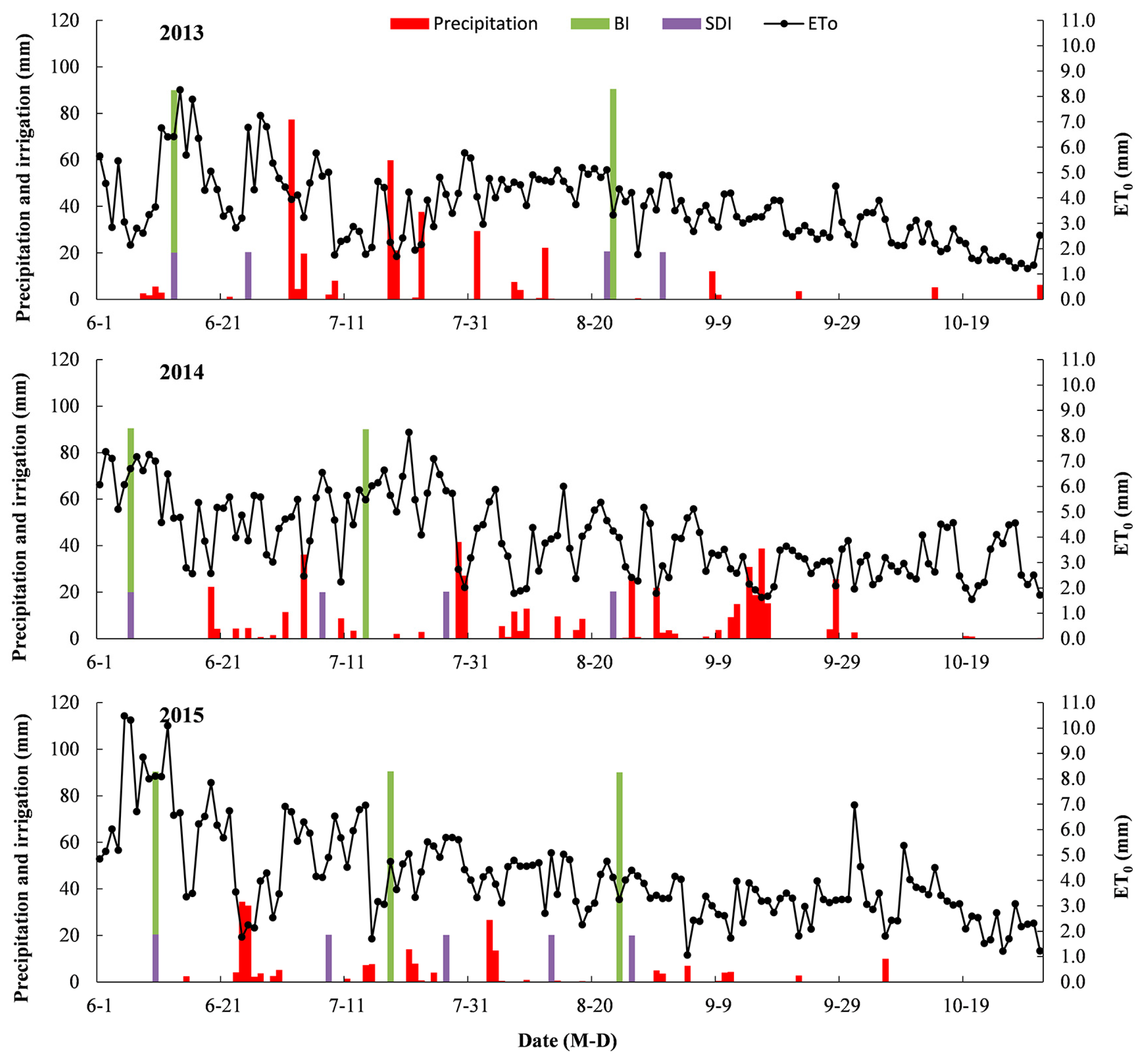
Field experiments were conducted at the Experimental Station of the Farmland Irrigation Research Institute located in Xinxiang (35°18′ N, 113°54′ E, 73.2 m above sea level), Henan Province, NCP, from May to October in 2013, 2014 and 2015. The site has a warm temperate climate with an annual mean air temperature of 14.2 °C, an annual sunshine duration of 2286 h, 220 frost-free days, a precipitation of 546 mm and a potential evaporation of 2000 mm based on the averages of 60-year data collected at the Xinxiang Weather Station near the experimental field. The groundwater table is more than 5 m deep at the experimental site. The physical properties of the soil at the experimental site are shown in Table 1. An automated wireless weather station (Vantage Pro2, Davis Instruments Co., Ltd., Hayward, CA, USA) was installed 50 m from the experimental field to monitor precipitation, air temperature, humidity, solar radiation and wind speed every 30 min. The precipitation and ET0 during the experimental seasons are shown in Figure 2.
2.1.2. Agronomic Practices
Cotton (Gossypium hirsutum L. cv. Zhongmiansuo 50) seedlings were raised in a greenhouse by sowing seeds in substrate (turf:vermiculite:perlite = 5:4:1). The seedlings were grown in separate soil blocks with a height of 35 mm and an inner diameter of 40 mm [3]. Several of the agronomic practices used are listed in Table 2. A rotary cultivator and a tray-seedling transplanter were used for ploughing the soil and for transplanting cotton seedlings after winter wheat harvest, respectively. Cotton was planted in rows extending south and north. The intervals between and within each row were 0.7 and 0.2 m, respectively. The plant population was 71,428 plants ha−1. A locally recommended fertilizer was used in the study for all treatments. The same rate and time of fertilizer application were used for the different irrigation methods. A compound fertilizer (N:P:K: 18, 18 and 18% composite) was applied at a rate of 70 kg ha−1 as the base fertilizer. The remaining N was applied at the squaring stage to achieve a rate of 60 kg ha−1 (urea, N 46%).
2.1.3. Experimental Design
The experiment was arranged in a completely randomized design with three replicates, and consisted of the BI and SDI treatments. The layout of the experimental plots is shown in Figure 3. The technical parameters of the irrigation methods are given in Table 3. The SDI systems were installed in the field after cotton was transplanted. The drip laterals were placed closer to each crop row, and each emitter was placed beside a plant.
Irrigation was conducted when the SWC in the root zone was depleted to 70% of field capacity (FC) during each of the three main plant growth periods (seedling stage, squaring stage, and bloom and boll-forming stage) [12,32,33]. SWC was calculated as the average value between the rows and inter-rows (0.35 m from the rows) of cotton plants. According to the characteristics of the different irrigation methods, 90 mm and 20 mm of irrigation water was applied in the BI and SDI treatments, respectively [34]. The amount of irrigation water applied in each treatment was measured using a water meter. Irrigation was first applied immediately after transplanting to ensure the survival of the cotton seedlings. The dates of irrigation are shown in Figure 2.
2.2. Measurement Methods
2.2.1. Root Spatial Distribution
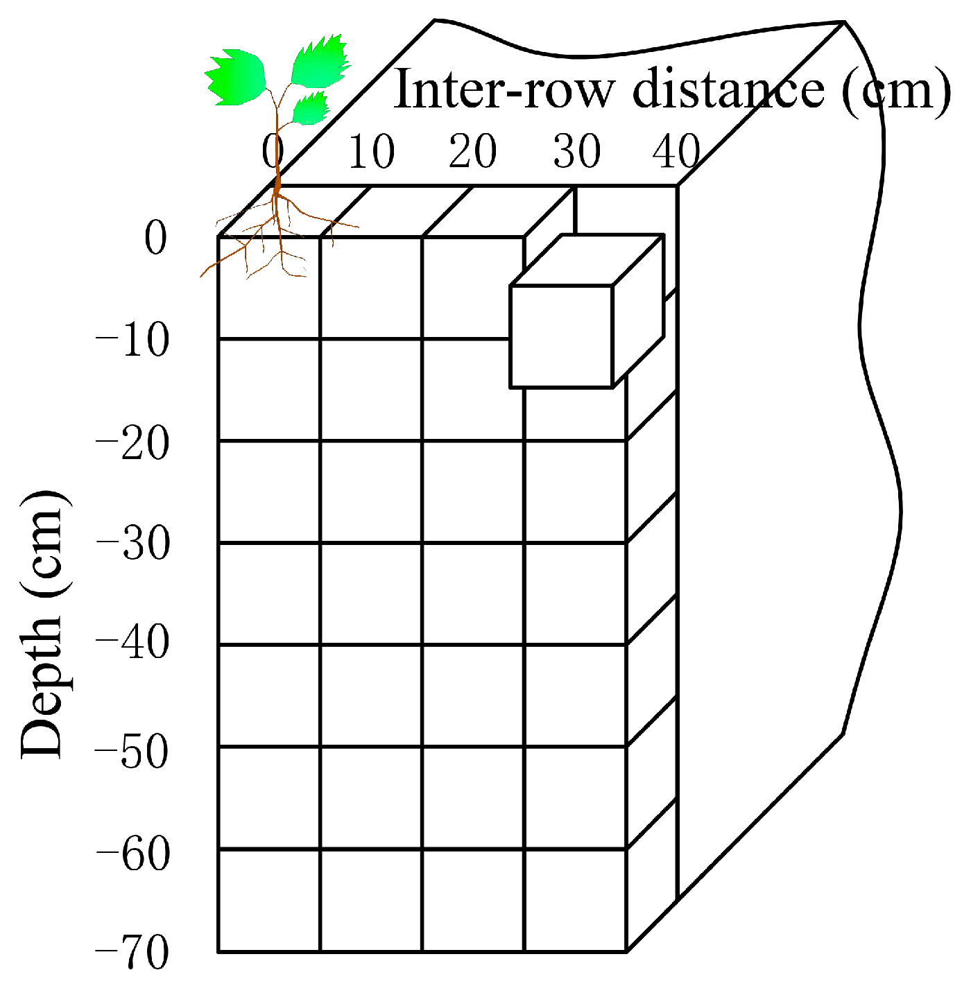
The two-dimensional root morphology and biomass distribution were determined using the soil core method [35]. According to the preliminary observations of the root systems of transplanted cotton reported by Mao et al. [10], the maximum root depth before blooming is less than 0.7 m. Therefore, we selected a location without weeds to dig 0.7 m-deep and 0.4 m-wide trenches, and pressed an iron box (10 × 10 × 10 cm) into the soil perpendicular to the soil profile to collect soil samples (Figure 4). Three sites (one in each treatment plot) were sampled per treatment during the course of one year. Because this method was destructive, we collected samples only during the critical periods of water use of the transplanted cotton (4 August 2013, 13 August 2014 and 16 August 2015). The collected soil samples were immediately soaked in freshwater for 6–8 h and washed in nylon mesh bags with 0.1 mm-diameter pores to select a root (diameter less than 2.5 mm) for subsequent analysis [36,37,38]. The selected root was scanned using a flatbed image scanner (Epson Perfection V700 PHOTO, Seiko Epson Co., Suwa, Nagano, Japan) to obtain root images and then dried in an oven at 80 °C until a constant weight was achieved to determine the root biomass. The root images were analysed using Win Rhizo Pro2007 software to determine the root length. The RLD and root biomass density (RBD) were determined by dividing the root length and root biomass by the soil sample volume (10 × 10 × 10 cm).
2.2.2. Dynamic Growth of the Root System
The dynamic growth of the root system was measured using the ET-100 root observation system (BTC. Bartz technology, Santa Barbara, CA, USA). We used WinRHIZO Tron software to obtain data by analysing the images of the root system. Minirhizotron tubes were installed at an angle of 45° from the ground using a matched soil auger in June 2013, and the angle of 45° was controlled by a matched protractor [39]. The minirhizotron tubes were 2 m long and installed in the rows and inter-rows (0.35 m from the rows) of the cotton plants. Six minirhizotron tubes (two in each treatment plot) were installed for each treatment. Observations were performed only when the surrounding soil environment became stable (approximately 12 months after installation) [40]. The RLD, root surface area density (RSAD), and root tip number density (RTND) were determined based on the root length, root surface area and number of root tips, which were each divided by the instrument observation area (1 × 1 cm) [36,37,41].
Because the period of July–August was a period of critical water demand for transplanted cotton, we observed root growth on the following dates: 16 July, 23 July, 28 July, 6 August, 14 August, 20 August and 25 August in 2014 and 17 July, 26 July, 6 August, 16 August, 23 August, 29 August, and 7 September in 2015.
2.2.3. Leaf Area and Plant Height
The leaf area and plant height were regularly measured using a leaf area metre (Li-3000, LI-COR, Lincoln, NE, USA) and a tape measure (accuracy of 0.1 cm), respectively [18]. The leaf area index (LAI) was then calculated using the Food and Agriculture Organization of the United Nations (FAO) method [42].
2.2.4. Soil Water Content (SWC)
The SWC (mm) was measured using time domain reflectometry with intelligent microelements (TRIME-PICO-IPH, IMKO Micromodultechnik GmbH, Ettlingen, Baden-Württemberg, Germany) from soil depths of 0 to 1 m at intervals of 0.2 m every 3–5 days. The SWC was calculated using gravimetric measurements [43]. The correction coefficients were uploaded to TRIME using TRIME WinCAL software. The TRIME tubes were installed in the rows and inter-rows (0.35 m from the rows) of the cotton plants using a soil auger. Six TRIME tubes (two in each treatment plot) were used in each treatment. The frequency of measurements was increased when the SWC in the root zone was nearly 70% of the Fc to ensure timely irrigation.
2.3. Numerical Modelling
2.3.1 Water Flow Equations
Soil water movement in the experiment field was simulated as the water flow in a 2D vertical plane. The governing equation for water flow was as follows [44]:
where θ is the volumetric water content (cm3·cm−3); t is the time (day); x and z are the distances from the origin in the x- and z-directions (cm), respectively; is the unsaturated hydraulic conductivity function (cm·day−1); is the unsaturated soil water diffusivity function (cm2·day−1); and is a sink term (day−1).
Soil hydraulic properties were estimated with the van Genuchten–Mualem function [45], as follows:
where is the saturated water content (cm3·cm−3); is the residual water content (cm3·cm−3); is the relative saturation; is the saturated hydraulic conductivity (cm·day−1); l is the pore connectivity parameter; , n and m are the shape parameters, and . The simulation domain was divided into five soil layers: 0–20, 20–40, 40–60, 60–80, and 80–100 cm. The soil input parameters are listed in Table 4.
2.3.2. Domain and Boundary Conditions
Figure 5 shows the domain geometry used in the HYDRUS-2D model to characterize BI and SDI in our experimental field. The domain geometry was defined as 35 cm in width and 100 cm in depth. In the BI treatment, the entire upper side of the domain was defined as the time-variable flux boundary to represent BI. In the SDI treatment, the left upper corner of the domain, which was 2.51 cm wide, was defined as the time-variable flux boundary to represent SDI. During irrigation, the fluxes of drip emitters were described in HYDRUS-2D as follows [18,21,23,25]:
where Q is the input irrigation flux (cm day−1); q is the discharge rate (2.0 L h−1); R is the radius of the drip emitter (0.8 cm); and L is the spacing between drip emitters (20 cm). The rest of the upper side of the domain in the SDI treatment was the atmospheric boundary condition representing the soil surface. The no-flux boundary was used on the right and left sides of the soil profile, because the relationship of the symmetry of the soil water pressure head inside and outside the geometry domain was assumed under both irrigation methods [19,20,25,26]. A free drainage boundary condition was imposed at the bottom of the soil profile.
2.3.3. Initial Conditions and Temporal and Spatial Discretization
The simulation experiment was conducted daily from transplanting to harvest. The SWCs measured before transplantation were used as the initial condition. The grid size in the top 30 cm was 1 cm; that between 30 and 60 cm was 3 cm; and that between 60 and 100 cm was 4 cm (Figure 5).
2.3.4. Estimating Evaporation and Transpiration
Evaporation from the exposed soil surface and potential transpiration were required as inputs in HYDRUS-2D. Both evaporation and transpiration were calculated daily using the dual crop coefficient approach of FAO-56 [46]. Under the dual crop coefficient approach, the evapotranspiration of the crop () was estimated using the following equation:
where Kcb is the basal crop coefficient; Ke is the soil water evaporation coefficient; and ET0 (cm) is the reference crop evapotranspiration computed via the FAO Penman–Monteith method [46]. Kcb is defined as the ratio of ETc/ET0 when the soil surface is dry but transpiration occurs at a potential rate. Ke represents the evaporation component from soil evaporation. Detailed information on the evaluation of these coefficients can be found in [46].
2.3.5. Root Water Uptake
In HYDRUS, the volume of water removed from the soil as a result of root water uptake is defined as follows [20]:
where α(h) is the soil water stress function (dimensionless) of Feddes et al. [47]; St is the length of the soil surface associated with transpiration (cm); is the potential transpiration rate (cm day−1); Xm and Zm are the maximum rooting lengths in the x- and z-directions (cm), respectively; and is the root distribution function developed by Vrugt et al. [48], which is as follows:
where px (-), pz (-), x* (cm), and z* (cm) are empirical parameters.
2.3.6. Model Calibration and Verification
In this study, the HYDRUS-2D model was calibrated using the measured SWCs in 2014. Saturated water content () and saturated hydraulic conductivity () were measured values, whereas , α and n were estimated via the ROSETTA pedotransfer functions [49] using a bulk density dataset and the particle size distribution. The parameters of the Feddes model were generated based on Forkutsa [50]: P0 = −10 cm, Popt = −25 cm, P2−1 = −200 cm, P2−2 = −600 cm, P3 = −14,000 cm. Root distribution was specified according to the RLD data measured using minirhizotrons. Then, the model was validated with the observed SWCs during the transplanted cotton-growing season in 2013–2015 without changing the calibrated parameters.
2.4. Statistical Analysis and Criteria of Model Evaluation
One-way analysis of variance (ANOVA) comparisons were made using the univariate general linear model (GLM) in SPSS Statistics 21.0, and the means were compared using least significant differences (LSD) after the ANOVA results were confirmed to be significant. The level of significance used for all statistical tests was p ≤ 0.05.
The following set of indicators was used to evaluate the agreement between the simulated results and the observed data for each treatment: root mean square error (RMSE) and model efficiency (EF). RMSE expresses the variance of the error; and EF is a normalized statistic that determines the relative magnitude of the residual variance compared with variance of the measured data [51,52].
where is a simulated value; is an observed value; n is the total number of observed values used in the calibration and validation processes; and are the mean values of the observed data points.
3. Results
3.1. Changes in Spatial Distribution of Root Length and Biomass
3.1.1. RLD Distribution
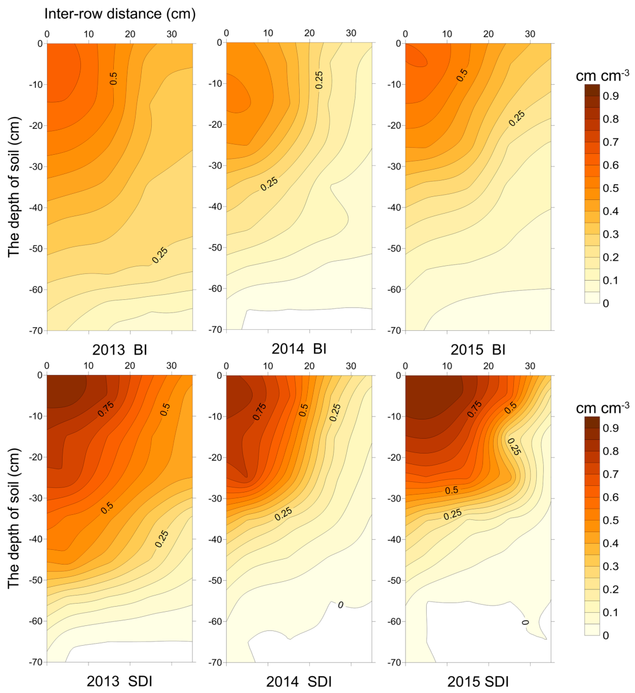
The spatial distribution of RLD at soil depths of 0–70 cm in the bloom and boll-forming stage of transplanted cotton is shown in Table 5 and Figure 6. In the BI treatment, the average RLD at depths of 0–70 cm ranged from 0.18 (in 2014) to 0.33 (in 2013) cm cm−3. The greatest RLDs were 0.47 cm cm−3 at soil depths of 0–10 cm in 2013; 0.31 cm cm−3 at soil depths of 10–20 cm in 2014; and 0.44 cm cm−3 at soil depths of 0–10 cm in 2015. A total of 57% (in 2013) to 71% (in 2015) of the total root length existed in the 0–30 cm soil layer. In the SDI treatment, the average RLD at depths of 0–70 cm ranged from 0.21 (in 2014) to 0.37 (in 2013) cm cm−3. The greatest RLDs, which were all observed at soil depths of 0–10 cm, were 0.67 (in 2013), 0.47 (in 2014) and 0.64 (in 2015) cm cm−3. A total of 69% (in 2013) to 89% (in 2015) of the total root length was observed in the 0–30 cm soil layer.
Compared with BI, SDI significantly increased the RLD in the –30 cm soil layer (p < 0.05). On average, for the three years of data, SDI increased the RLD in the 0–30 cm soil layer by 39% and decreased RLD in the 30–70 cm soil layer by 31% compared with BI.
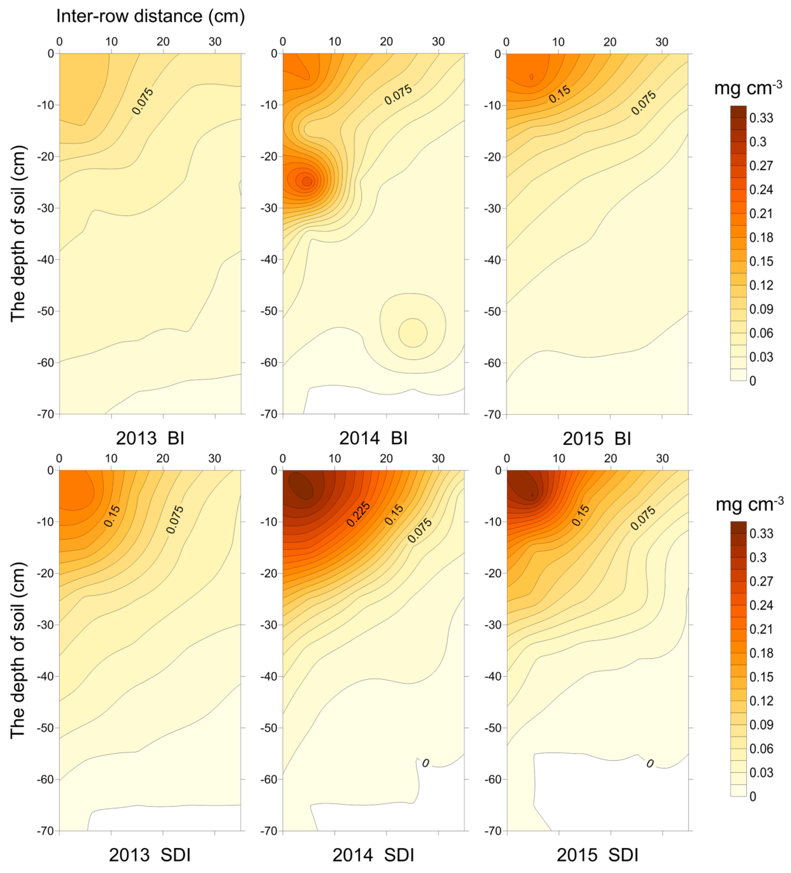
3.1.2. RBD Distribution
The spatial distribution of the RBD at soil depths of 0–70 cm in the bloom and boll-forming stage of transplanted cotton is shown in Table 6 and Figure 7. The distribution of RBD was similar to that of RLD. In the BI treatment, the average RBD at depths of 0–70 cm ranged from 0.043 (in 2013) to 0.46 (in 2014) mg cm−3. The highest RBDs, all of which were observed at soil depths of 0–10 cm, were 0.082 (in 2013), 0.108 (in 2014) and 0.129 (in 2015) mg cm−3. A total of 63% (in 2013) to 78% (in 2015) of the total root biomass was observed in the 0–30 cm soil layer. In the SDI treatment, the average RBD at depths of 0–70 cm ranged from 0.046 (in 2013) to 0.058 (in 2014) mg cm−3. The highest RBDs, all of which were observed at soil depths of 0–10 cm, were 0.111 (in 2013), 0.191 (in 2014) and 0.164 (in 2015) mg cm−3. A total of 78% (in 2013) to 90% (in 2015) of the total root biomass was observed in the 0–30 cm soil layer.
Compared with BI, SDI significantly increased the RBD in the 0–30 cm soil layer (p < 0.05). On average, for the three years of data, SDI increased RBD in the 0–30 cm soil layer by 37% and decreased RLD in the 30–70 cm soil layer by 42% compared with BI.
3.2. Growth of Root System
3.2.1. Variations in RLD, RSAD, RTND and Root Diameter (RD)
Figure 8 and Figure 9 show the changes in the mean values of RLD, RSAD, RTND and root diameter (RD) in transplanted cotton in 2014 and 2015. In the SDI treatment, the greatest RLD (0.38 cm cm−2), RSAD (0.035 cm2 cm−2) and RTND (0.60 tips cm−2) were all observed on 6 August (61 days after planting) in 2014, and the greatest RLD (0.40 cm cm−2), RSAD (0.034 cm2 cm−2) and RTND (0.80 tips cm−2) were observed on 16 August (67 days after planting) in 2015. RD increased monotonically with the growth of the root system. In the BI treatment, the greatest RLD, RSAD and RTND were 0.20 cm cm−2, 0.016 cm2 cm−2 and 0.42 tips cm−2 , respectively, in 2014, and 0.28 cm cm−2, 0.017 cm2 cm−2 and 0.52 tips cm−2, respectively, in 2015.
On average, for the two years of data, SDI increased the RD, RLD, RSAD and RTND by 19%, 69%, 118% and 69%, respectively, compared with BI. In the BI treatment, the RLD, RSAD and RTND fluctuated for up to 61 days after transplantation and showed slight reductions at some times, whereas in the SDI treatment, these parameters increased continuously.
3.2.2. Two-Dimensional Model of RLD Parameters
The RLD(x, z, t) root parameters under the normalized root water uptake distribution in HYDRUS-2D were defined using the observations of RLD obtained using minirhizotrons. Because HYDRUS-2D software assumed that the root distribution was constant throughout the entire growth period, the parameters of Equation (8) were input according to the different growth stages of transplanted cotton. The estimated RLD parameters for different growth stages of transplanted cotton are shown in Table 7.
3.3. Simulation of Soil Water Movement
3.3.1. Model Evaluation
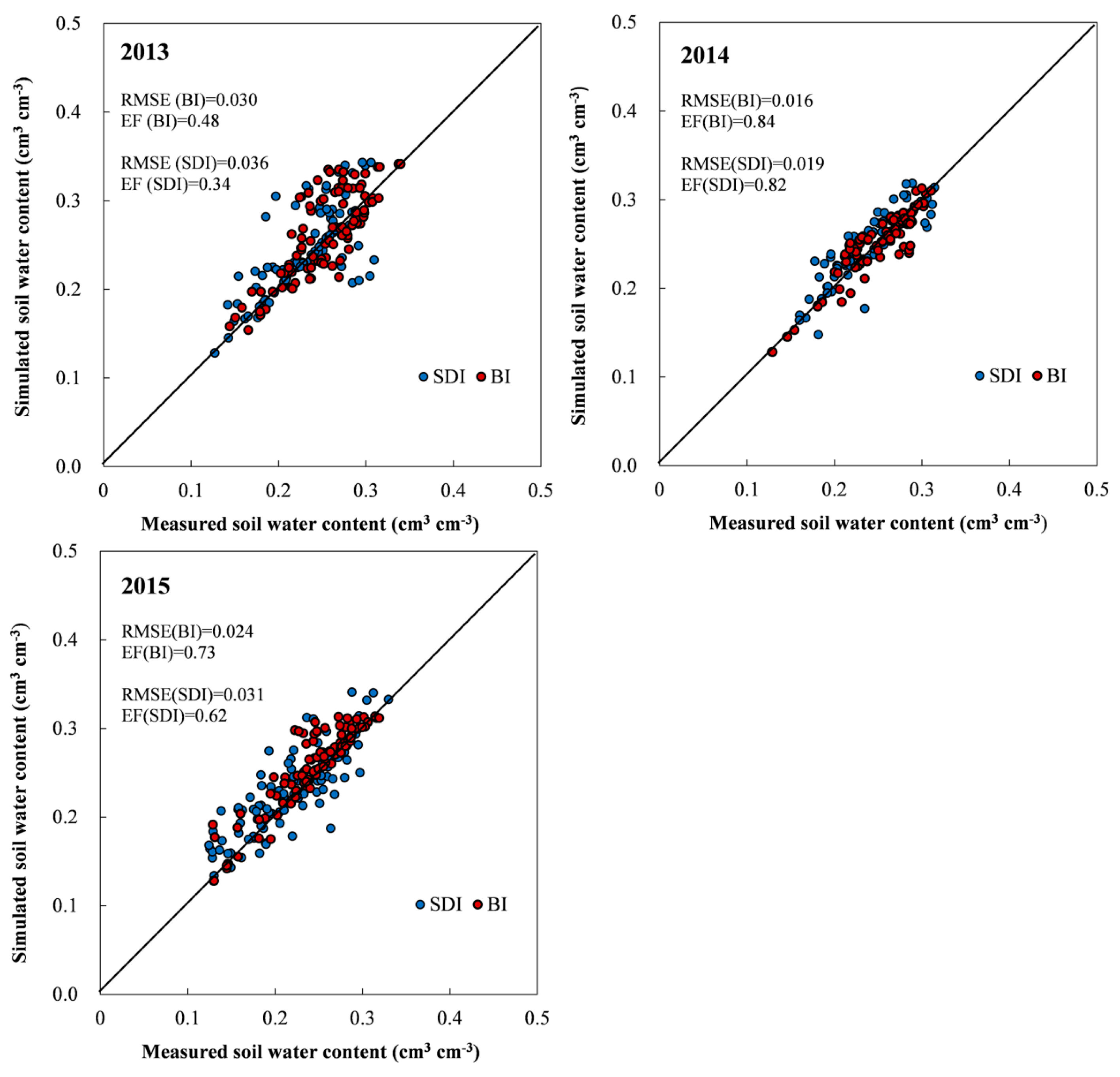
The “goodness-of-fit” indicators and scatter plots between the simulated results and the observations of the SWCs are shown in Figure 10. Good agreement was found between the simulated and measured SWCs. On average, for all three years of data, the RMSEs of the BI and SDI treatments were 0.023 and 0.029 cm3 cm−3, respectively, with corresponding EFs of 0.68 and 0.59. These RMSE values are in the range and smaller than those reported by Li et al. [53] (RMSE values ranging from 0.031 to 0.046 cm3 cm−3) and by Li et al. [18] (RMSE values ranging from 0.035 to 0.043 cm3 cm−3). High EF values were also obtained, indicating that the residual variance was smaller than the measured data variance. Based on these values, it can be concluded that the correspondence between simulations and observations was very good.
3.3.2. Simulation of Soil Water Movement
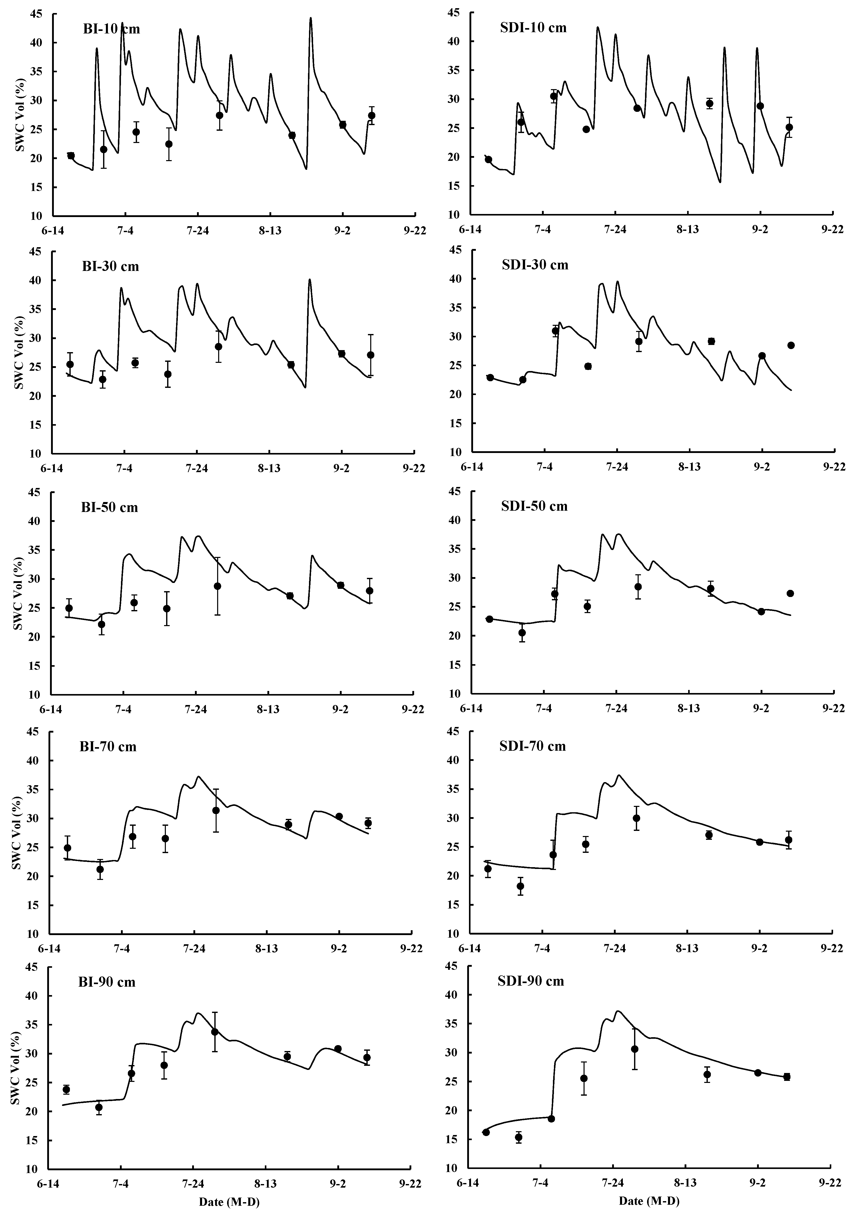
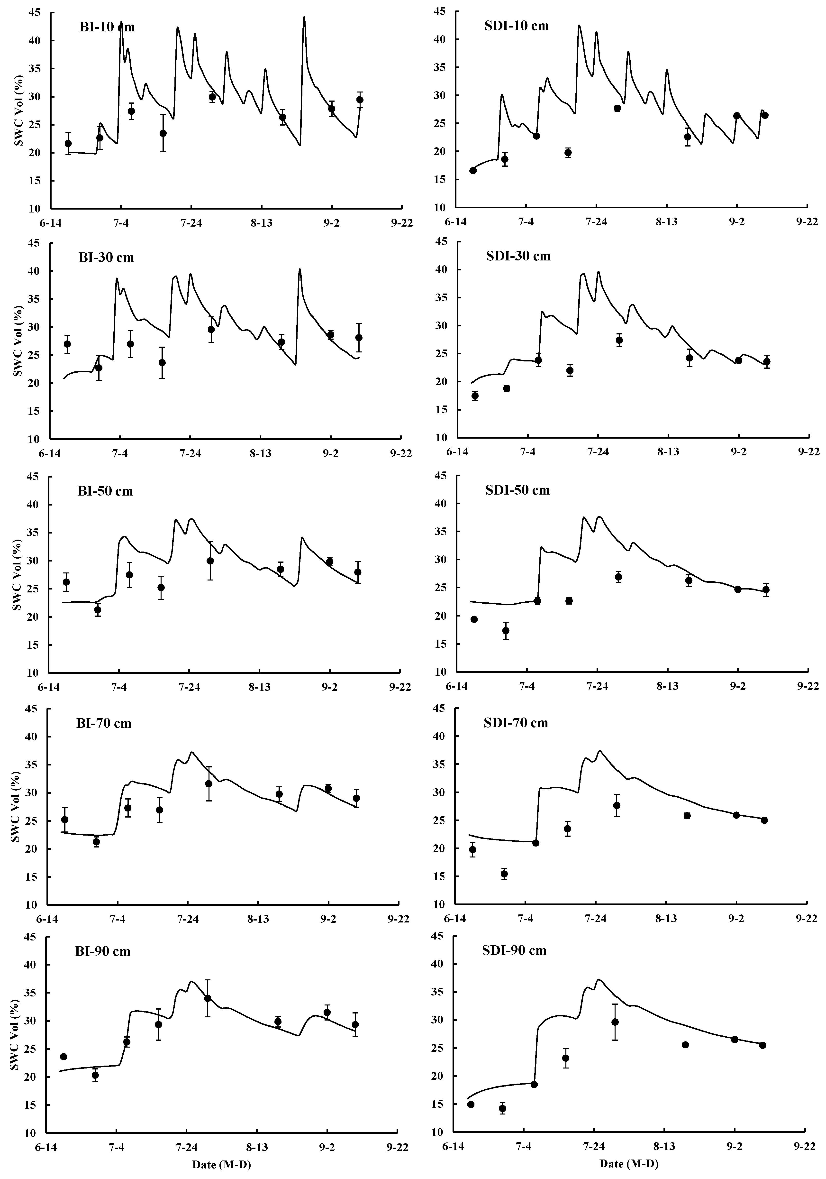
Since similar trends in the SWCs were observed during the three years, we could select only one-year data to present the simulation of soil water movement. To explore the reason for the relative poor fit of the simulation in 2013, the simulated and observed SWCs for 2013 are presented in Figure 11 and Figure 12. Figure 11 and Figure 12 represent different horizontal locations: Figure 11 corresponds to the point in the cotton planting rows, and Figure 12 to the point in the middle of the inter-rows (0.35 m from the rows). The two columns in the plots represent the two different irrigation methods (BI and SDI), and the five rows represent the following depths from the soil surface: 10, 30, 50, 70 and 90 cm.
Although the accuracy of the simulation was the lowest for 2013, both Figure 11 and Figure 12 show that the simulated SWC values were still in close agreement with the observed values. Furthermore, the fluctuation patterns of the SWC that resulted from the irrigation and precipitation events were consistent.
In the BI treatment, the average observed SWC in the cotton planting rows (0.26 cm3 cm−3) and that in the middle of the inter-rows (0.27 cm3 cm−3) were roughly the same. The simulated values showed that BI could saturate the soil in the 0–30 cm layer and dampen the soil in the 30–90 cm layer. The SWC changes in the upper layer were clearly more drastic than those in the deeper layer. The SWCs at 0–30 cm fluctuated, ranging from 0.18 to 0.44 cm3 cm−3, whereas the SWCs at 30–90 cm ranged from 0.21 to 0.37 cm3 cm−3. In the SDI treatment, the average observed SWC in the cotton planting rows was 0.25 cm3 cm−3, which was 12% higher than that in the middle of the inter-rows. The simulated values showed that SDI could only saturate soil in the 0–10 cm layer and dampen soil in the 10–30 cm layer, suggesting that the applied SDI does not result in significant periodical changes for the SWCs below 30 cm. The average SWC observed at 30–90 cm in the SDI treatment was 0.28 cm3 cm−3, which was 5% lower than that in the BI treatment.
4. Discussion
4.1. Root Characteristics of Transplanted Cotton
Roots are closely related to soil water movement; therefore, investigating the deformed root distribution of transplanted cotton is essential for simulating soil water movement under different irrigation methods. Three main differences were observed in the root systems of transplanted and direct-seeded cotton. (1) The root systems of transplanted cotton are significantly damaged, with many fine roots being lost when the cotton is transplanted into the field. This root damage decreases the ability of transplanted cotton to absorb moisture and nutrients; (2) After transplantation, the growth environment of the roots changes from a substrate containing high levels of nutrients and moisture in the seedling greenhouse to relatively poor soil in the field [3,4]. Therefore, the speed and quality of root recovery after transplantation are important factors that affect the root water uptake and yield of transplanted cotton; (3) The root systems of direct-seeded cotton are arranged in the shape of an inverted cone, whereas the roots of transplanted cotton are arranged in the shape of a claw [10]. Although cotton is a woody plant, the taproot of transplanted cotton has degenerated because the roots of transplanted cotton are malformed from binding to the seedling aperture disk before transplantation. Lateral roots occupy the position of the taproot in the root system of transplanted cotton. According to studies examining the roots of direct-seeded cotton and the results of this study, the RLD of transplanted cotton is higher at soil depths of 0–0.3 m and lower at depths below 0.3 m than that of direct-seeded cotton [10,13].
These differences indicate that the root development of transplanted cotton must be investigated under different irrigation methods, which is an important step for simulating soil water movement in transplanted cotton fields.
4.2. Effects of Soil Water Movement on Root Development of Transplanted Cotton under Different Irrigation Methods
This study showed that the soil water movement occurring under different irrigation methods has a significant influence on the deformed roots of transplanted cotton. Compared with BI, SDI increased the RLD and RBD in the 0–0.3 m soil layer (Figure 6 and Figure 7) by improving the soil environment at these soil depths, which is advantageous for the root growth of transplanted cotton [54]. Primarily, the SWC in the SDI treatment was particularly suitable for the root growth of transplanted cotton. Hu et al. [12] indicated that cotton roots grow quickly when the SWC is near 75% of FC, but slowly when the SWC is near 90% or 60% of FC. SDI concentrated the root system of transplanted cotton in the soil maintained at a relatively stable water content. Therefore, the root system in the SDI treatment suffered from less stress than the root systems in the BI treatment, in which the SWC fluctuated between water deficit conditions before irrigation and waterlogged conditions after irrigation, especially in the 0–0.3 m soil layer [14,55]. Secondly, the amount of irrigation in the SDI treatment was sufficiently low to prevent deep infiltration, reducing the loss of nutrients [13]. BI resulted in more rapid leaching of chemicals than SDI, which led to different nutrient distribution patterns and variations in the growth and profile distribution of roots [56,57]. Finally, in the SDI treatment, the drip emitters were near the soil surface, which resulted in minimal damage to the topsoil structure and therefore was advantageous for gas exchange between the soil and the atmosphere [14,55]. However, in the BI treatment, the number of unsaturated soil pores was reduced after irrigation, which inhibited the exchange of gas between the soil and atmosphere, and consequently obstructed the respiration of cotton roots [58]. Concurrently, the large amount of water applied by BI decreased the activity of cotton roots, because the cotton cannot tolerate waterlogged conditions [11,14].
4.3. Modeling Soil Water Movement under Different Irrigation Methods
The simulation of SWCs at different soil depths and horizontal locations in transplanted cotton fields irrigated by BI and SDI has been accomplished with the modeling study. This modeling study can help optimize irrigation strategies and improve irrigation water use efficiency in the transplanted cotton field irrigated by BI and SDI. The estimation of the vertical wetting front advance allows the calculation of the optimum irrigation time to minimize deep percolation of water below the root zone and prevent the loss of soluble nutrients into groundwater [59].
The results of the simulation model suggested that the observed SWCs and the simulated results obtained with HYDRUS-2D were in good agreement (Figure 10). Overall, the changes in the simulated SWCs at 0–30 cm were more drastic than those at 30–90 cm in both irrigation treatments (Figure 11 and Figure 12), since the 0–30 cm layer is more directly affected by irrigation, precipitation, evaporation, and transpiration [21,24]. The simulation results in Figure 11 and Figure 12 showed that the HYDRUS-2D model overestimated the SWCs in July 2013. This was maybe due to the bias of the model output caused by the heavy, frequent and continuous rainfall in July 2013. In July 2013, the maximum rainfall intensity was 77.3 mm/d (2 July 2013), and the total precipitation was 231.1 mm, while the precipitation during the same period in 2014 and 2015 was only 134.5 and 43.5 mm, respectively (Figure 2). The HYDRUS-2D model and the dual crop coefficient approach of FAO-56 were calibrated using the measured data in 2014, and produced a cumulative bias under the extreme rainfall conditions in 2013. Nevertheless, the simulated and measured results in 2013 still exhibited highly consistent trends, with several consecutive irrigation and precipitation events in the transplanted cotton growing seasons, particularly considering the complexity of the conditions to which the model was applied (i.e., heterogeneous soil properties, a more than 120-day simulation period, high evaporative demand, and assumed constant root distribution in one growth stage) [21,24].
5. Conclusions
This study showed that SDI was well suited for producing the optimal soil water distribution pattern for the deformed root system of transplanted cotton, and the root system of transplanted cotton was more developed under SDI than under BI. The HYDRUS-2D model can be applied to a transplanted cotton field irrigated by BI or SDI for modeling the SWC, and the simulated values of the SWC were in close agreement with the observed values.
Acknowledgments
We acknowledge financial support from the China Agriculture Research System (CARS-18-19), the Special Fund for Agro-Scientific Research in the Public Interest (201203077) and the Special Fund for the Public Interest of the Ministry of Water Resources (201501017).
Author Contributions
The research presented here was conducted in collaboration among all authors. Hao Zhang, Hao Liu and Jingsheng Sun conceived and designed the study; Hao Zhang conducted the data analysis and prepared the first draft of the manuscript; Chitao Sun, Yang Gao, Xuewen Gong, Jingsheng Sun and Wanning Wang provided important advice on the concept of the methodology and the writing of the manuscript.
Conflicts of Interest
The authors declare no conflict of interest.
References
- Dong, H.Z.; Li, W.J.; Tang, W.; Li, Z.H.; Zhang, D.W.; Niu, Y.H. Yield, quality and leaf senescence of cotton grown at varying planting dates and plant densities in the Yellow River Valley of China. Field Crops Res. 2006, 98, 106–115. [Google Scholar] [CrossRef]
- CRI (Cotton Research Institute Chinese Academy of Agricultural Sciences). Cultivation of Cotton in China; Shanghai Science and Technology Press: Shanghai, China, 2013. [Google Scholar]
- Dong, H.Z.; Li, W.J.; Tang, W.; Li, Z.H.; Zhang, D.M. Enhanced plant growth, development and fiber yield of Bt transgenic cotton by an integration of plastic mulching and seedling transplanting. Ind. Crops Prod. 2007, 26, 298–306. [Google Scholar] [CrossRef]
- Dong, H.Z.; Li, W.J.; Tang, W.; Li, Z.H.; Zhang, D.M. Increased yield and revenue with a seedling transplanting system for hybrid seed production in Bt cotton. J. Agron. Crop Sci. 2005, 191, 116–124. [Google Scholar] [CrossRef]
- Zhang, L.; van der Werf, W.; Zhang, S.; Li, B.; Spiertz, J.H.J. Growth, yield and quality of wheat and cotton in relay strip intercropping systems. Field Crops Res. 2007, 103, 178–188. [Google Scholar] [CrossRef]
- Zhang, L.; van der Werf, W.; Bastiaans, L.; Zhang, S.; Li, B.; Spiertz, J.H.J. Light interception and utilization in relay intercrops of wheat and cotton. Field Crops Res. 2008, 107, 29–42. [Google Scholar] [CrossRef]
- Dai, J.L.; Dong, H.Z. Intensive cotton farming technologies in China: Achievements, challenges and countermeasures. Field Crops Res. 2014, 155, 99–110. [Google Scholar] [CrossRef]
- Luo, H.H.; Tao, X.P.; Hu, Y.Y.; Zhang, Y.L.; Zhang, W.F. Response of cotton root growth and yield to root restriction under various water and nitrogen regimes. J. Plant Nutr. Soil Sci. 2015, 178, 384–392. [Google Scholar] [CrossRef]
- Xu, X.; Huang, G.H.; Qu, Z.Y.; Pereira, L.S. Assessing the groundwater dynamics and impacts of water saving in the Hetao Irrigation District, Yellow River basin. Agric. Water Manag. 2010, 98, 301–313. [Google Scholar] [CrossRef]
- Mao, S.C.; Li, P.C.; Han, Y.C.; Wang, G.P.; Li, Y.B.; Wang, X.H. Preliminary Observation on Morphological Parameters of Root System of the Root-naked Transplanting Cotton (Gossypium hirsutum L.). Cotton Sci. 2008, 20, 76–78. [Google Scholar]
- Hulugalle, N.R.; Broughton, K.J.; Tan, D.K.Y. Fine root production and mortality in irrigated cotton, maize and sorghum sown in vertisols of northern New South Wales, Australia. Soil Tillage Res. 2015, 146, 313–322. [Google Scholar] [CrossRef]
- Hu, X.T.; Chen, H.; Wang, J.; Meng, X.B.; Chen, F.H. Effects of Soil Water Content on Cotton Root Growth and Distribution Under Mulched Drip Irrigation. Agric. Sci. China 2009, 8, 709–716. [Google Scholar] [CrossRef]
- Ning, S.R.; Shi, J.C.; Zuo, Q.; Wang, S.; Ben-Gal, A. Generalization of the root length density distribution of cotton under film mulched drip irrigation. Field Crops Res. 2015, 177, 125–136. [Google Scholar] [CrossRef]
- Hodgson, A.S.; Constable, G.A.; Duddy, G.R.; Daniells, I.G. A comparison of drip and furrow irrigated cotton on a cracking clay soil. 2. Water use efficiency, waterlogging, root distribution and soil structure. Irrig. Sci. 1990, 11, 143–148. [Google Scholar] [CrossRef]
- Rao, S.S.; Tanwar, S.P.S.; Regar, P.L. Effect of deficit irrigation, phosphorous inoculation and cycocel spray on root growth, seed cotton yield and water productivity of drip irrigated cotton in arid environment. Agric. Water Manag. 2016, 169, 14–25. [Google Scholar] [CrossRef]
- Sampathkumar, T.; Pandian, B.J.; Mahimairaja, S. Soil moisture distribution and root characters as influenced by deficit irrigation through drip system in cotton–maize cropping sequence. Agric. Water Manag. 2012, 103, 43–53. [Google Scholar] [CrossRef]
- Min, W.; Guo, H.J.; Zhou, G.W.; Zhang, W.; Ma, L.J.; Ye, J.; Hou, Z.N. Root distribution and growth of cotton as affected by drip irrigation with saline water. Field Crops Res. 2014, 169, 1–10. [Google Scholar] [CrossRef]
- Li, X.Y.; Shi, H.B.; Šimůnek, J.; Gong, X.W.; Peng, Z.Y. Modeling soil water dynamics in a drip-irrigated intercropping field under plastic mulch. Irrig. Sci. 2015, 33, 289–302. [Google Scholar] [CrossRef]
- Provenzano, G. Using HYDRUS-2D simulation model to evaluate wetted soil volume in subsurface drip irrigation systems. J. Irrig. Drain. Eng. 2007, 133, 342–349. [Google Scholar] [CrossRef]
- Šimůnek, J.; Sejna, M.; Genuchten, M.T.V. The HYDRUS Software Package for Simulating Two-and Three-Dimensional Movement of Water, Heat, and Multiple Solutes in Variable-Saturated Media; User Manual, Version 1.0; PC Progress: Prague, Czech Republic, 2006. [Google Scholar]
- Bufon, V.B.; Lascano, R.J.; Bednarz, C.; Booker, J.D.; Gitz, D.C. Soil water content on drip irrigated cotton: Comparison of measured and simulated values obtained with the Hydrus 2-D model. Irrig. Sci. 2012, 30, 259–273. [Google Scholar] [CrossRef]
- Kandelous, M.M.; ŠImůNek, J. Numerical simulations of water movement in a subsurface drip irrigation system under field and laboratory conditions using HYDRUS-2D. Agric. Water Manag. 2010, 97, 1070–1076. [Google Scholar] [CrossRef]
- Phogat, V.; Mahadevan, M.; Skewes, M.; Cox, J.W. Modelling soil water and salt dynamics under pulsed and continuous surface drip irrigation of almond and implications of system design. Irrig. Sci. 2012, 30, 315–333. [Google Scholar] [CrossRef]
- Han, M.; Zhao, C.Y.; Feng, G.; Yan, Y.Y.; Sheng, Y. Evaluating the Effects of Mulch and Irrigation Amount on Soil Water Distribution and Root Zone Water Balance Using HYDRUS-2D. Water 2015, 7, 2622–2640. [Google Scholar] [CrossRef]
- Trout, T.J.; ŠImůNek, J.; Shouse, P.J.; Skaggs, T.H. Comparison of HYDRUS-2D Simulations of Drip Irrigation with Experimental Observations. J. Irrig. Drain. Eng. 2004, 130, 304–310. [Google Scholar]
- Mguidiche, A.; Provenzano, G.; Douh, B.; Khila, S.; Rallo, G.; Boujelben, A. Assessing Hydrus-2D to Simulate Soil Water Content (SWC) and Salt Accumulation Under an SDI System: Application to a Potato Crop in a Semi-Arid Area of Central Tunisia. Irrig. Drain. 2015, 64, 263–274. [Google Scholar] [CrossRef]
- Zhang, Y.Y.; Wu, P.T.; Zhao, X.N.; Wang, Z.K. Simulation of soil water dynamics for uncropped ridges and furrows under irrigation conditions. Can. J. Soil Sci. 2017, 93, 85–98. [Google Scholar] [CrossRef]
- Chen, L.J.; Feng, Q.; Li, F.R.; Li, C.S. Simulation of soil water and salt transfer under mulched furrow irrigation with saline water. Geoderma 2014, 241–242, 87–96. [Google Scholar] [CrossRef]
- Crevoisier, D.; Popova, Z.; Mailhol, J.C.; Ruelle, P. Assessment and simulation of water and nitrogen transfer under furrow irrigation. Agric. Water Manag. 2008, 95, 354–366. [Google Scholar] [CrossRef]
- Kang, Y.H.; Wang, R.S.; Wan, S.Q.; Hu, W.; Jiang, S.F.; Liu, S.P. Effects of different water levels on cotton growth and water use through drip irrigation in an arid region with saline ground water of Northwest China. Agric. Water Manag. 2012, 109, 117–126. [Google Scholar] [CrossRef]
- Cetin, O.; Bilgel, L. Effects of different irrigation methods on shedding and yield of cotton. Agric. Water Manag. 2002, 54, 1–15. [Google Scholar] [CrossRef]
- Ibragimov, N.; Evett, S.R.; Esanbekov, Y.; Kamilov, B.S.; Mirzaev, L.; Lamers, J.P.A. Water use efficiency of irrigated cotton in Uzbekistan under drip and furrow irrigation. Agric. Water Manag. 2007, 90, 112–120. [Google Scholar] [CrossRef]
- Guan, H.J.; Li, J.S.; Li, Y.F. Effects of drip system uniformity and irrigation amount on cotton yield and quality under arid conditions. Agric. Water Manag. 2013, 124, 37–51. [Google Scholar] [CrossRef]
- Lv, G.H.; Kang, Y.H.; Li, L.; Wan, S.Q. Effect of irrigation methods on root development and profile soil water uptake in winter wheat. Irrig. Sci. 2010, 28, 387–398. [Google Scholar] [CrossRef]
- Salgado, E.; Cautín, R. Avocado root distribution in fine and coarse-textured soils under drip and microsprinkler irrigation. Agric. Water Manag. 2008, 95, 817–824. [Google Scholar] [CrossRef]
- Kage, H.; Kochler, M.; Stutzel, H. Root growth of cauliflower (Brassica oleracea L. botrytis) under unstressed conditions: Measurement and modelling. Plant Soil 2000, 223, 131–145. [Google Scholar]
- Jose, S.; Gillespie, A.R.; Seifert, J.R.; Pope, P.E. Comparison of minirhizotron and soil core methods for quantifying root biomass in a temperate alley cropping system. Agrofor. Syst. 2001, 52, 161–168. [Google Scholar] [CrossRef]
- Li, C.X.; Zhou, X.G.; Sun, J.S.; Wang, H.Z.; Gao, Y. Dynamics of root water uptake and water use efficiency under alternate partial root-zone irrigation. Desalin. Water Treat. 2014, 52, 2805–2810. [Google Scholar] [CrossRef]
- Bragg, P.L.; Govi, G.; Cannell, R.Q. A comparison of methods, including angled and vertical minirhizotrons, for studying root growth and distribution in a spring oat crop. Plant Soil 1983, 73, 435–440. [Google Scholar] [CrossRef]
- Johnson, M.G.; Tingey, D.T.; Phillips, D.L.; Storm, M.J. Advancing fine root research with minirhizotrons. Environ. Exp. Bot. 2001, 45, 263–289. [Google Scholar] [CrossRef]
- Li, C.X.; Sun, J.S.; Li, F.S.; Zhou, X.G.; Li, Z.Y.; Qiang, X.M.; Guo, D.D. Response of root morphology and distribution in maize to alternate furrow irrigation. Agric. Water Manag. 2011, 98, 1789–1798. [Google Scholar] [CrossRef]
- Allen, R.G.; Pereira, L.S.; Raes, D.; Smith, M. Crop Evapotranspiration–Guidelines for Computing Crop Water Requirements–FAO Irrigation and Drainage Paper 56; Food and Agriculture Organization of the United Nations: Rome, Italy, 1998. [Google Scholar]
- Weitz, A.M.; Grauel, W.T.; Keller, M.; Veldkamp, E. Calibration of time domain reflectometry technique using undisturbed soil samples from humid tropical soils of volcanic origin. Water Resour. Res. 1997, 33, 1241–1249. [Google Scholar] [CrossRef]
- Richards, L.A. Capillary conduction of liguids through porous mediums. Physics 1931, 1, 318–333. [Google Scholar] [CrossRef]
- Van Genuchten, M.T. A closed-form equation for predicting the hydraulic conductivity of unsaturated soils. Soil Sci. Soc. Am. J. 1980, 44, 892–898. [Google Scholar] [CrossRef]
- Allen, R.G.; Smith, M.; Wright, J.L.; Raes, D.; Pereira, L.S. FAO-56 Dual Crop Coefficient Method for Estimating Evaporation from Soil and Application Extensions. J. Irrig. Drain. Eng. 2005, 131, 2–13. [Google Scholar] [CrossRef]
- Feddes, R.A.; Kowalik, P.J.; Zaradny, H. Simulation of field water use and crop yield. Soil Sci. 1982, 129, 193. [Google Scholar]
- Vrugt, J.A.; Hopmans, J.W.; Šimunek, J. Calibration of a Two-Dimensional Root Water Uptake Model. Fluid Phase Equilib. 2001, 65, 1027–1037. [Google Scholar] [CrossRef]
- Schaap, M.G.; Leij, F.J.; Genuchten, M.T.V. A computer program for estimating soil hydraulic parameters with hierarchical pedotransfer functions. J. Hydrol. 2001, 251, 163–176. [Google Scholar] [CrossRef]
- Forkutsa, I.; Sommer, R.; Shirokova, Y.I.; Lamers, J.P.A.; Kienzler, K.; Tischbein, B.; Martius, C.; Vlek, P.L.G. Modeling irrigated cotton with shallow groundwater in the Aral Sea Basin of Uzbekistan: II. Soil salinity dynamics. Irrig. Sci. 2009, 27, 319–330. [Google Scholar] [CrossRef]
- Paredes, P.; de Melo-Abreu, J.P.; Alves, I.; Pereira, L.S. Assessing the performance of the FAO AquaCrop model to estimate maize yields and water use under full and deficit irrigation with focus on model parameterization. Agric. Water Manag. 2014, 144, 81–97. [Google Scholar] [CrossRef]
- Moriasi, D.N.; Arnold, J.G.; Van Liew, M.W.; Bingner, R.L.; Harmel, R.D.; Veith, T.L. Model evaluation guidelines for systematic quantification of accuracy in watershed simulations. Trans. Asabe 2007, 50, 885–900. [Google Scholar] [CrossRef]
- Li, H.J.; Yi, J.; Zhang, J.G.; Zhao, Y.; Si, B.C.; Hill, R.L.; Cui, L.; Liu, X.Y. Modeling of Soil Water and Salt Dynamics and Its Effects on Root Water Uptake in Heihe Arid Wetland, Gansu, China. Water 2015, 7, 2382–2401. [Google Scholar] [CrossRef]
- Qu, L.Y.; Quoreshi, A.M.; Koike, T. Root growth characteristics, biomass and nutrient dynamics of seedlings of two larch species raised under different fertilization regimes. Plant Soil 2003, 255, 293–302. [Google Scholar] [CrossRef]
- Lv, G.H.; Song, J.Q.; Bai, W.B.; Wu, Y.F.; Liu, Y.; Kang, Y.H. Effects of different irrigation methods on micro-environments and root distribution in winter wheat fields. J. Integr. Agric. 2015, 14, 1658–1672. [Google Scholar]
- Zaman, W.Z.; Arshad, M.; Saleem, A. Distribution of nitrate-nitrogen in the soil profile under different irrigation methods. Int. J. Agric. Biol. 2001, 3, 208–209. [Google Scholar]
- Home, P.G.; Panda, R.K.; Kar, S. Effect of method and scheduling of irrigation on water and nitrogen use efficiencies of Okra (Abelmoschus esculentus). Agric. Water Manag. 2002, 55, 159–170. [Google Scholar] [CrossRef]
- Yu, Y.X.; Zhao, C.Y.; Zhao, Z.M.; Yu, B.; Zhou, T.H. Soil respiration and the contribution of root respiration of cotton (Gossypium hirsutum L.) in arid region. Acta Ecol. Sin. 2015, 35, 17–21. [Google Scholar] [CrossRef]
- Elmaloglou, S.; Diamantopoulos, E. Simulation of soil water dynamics under subsurface drip irrigation from line sources. Water Resour. Manag. 2013, 27, 4131–4148. [Google Scholar] [CrossRef]
Figure 1.
Root morphologies resulting from different planting patterns (transplanted cotton on the left, direct-seeded cotton on the right).
Figure 1.
Root morphologies resulting from different planting patterns (transplanted cotton on the left, direct-seeded cotton on the right).
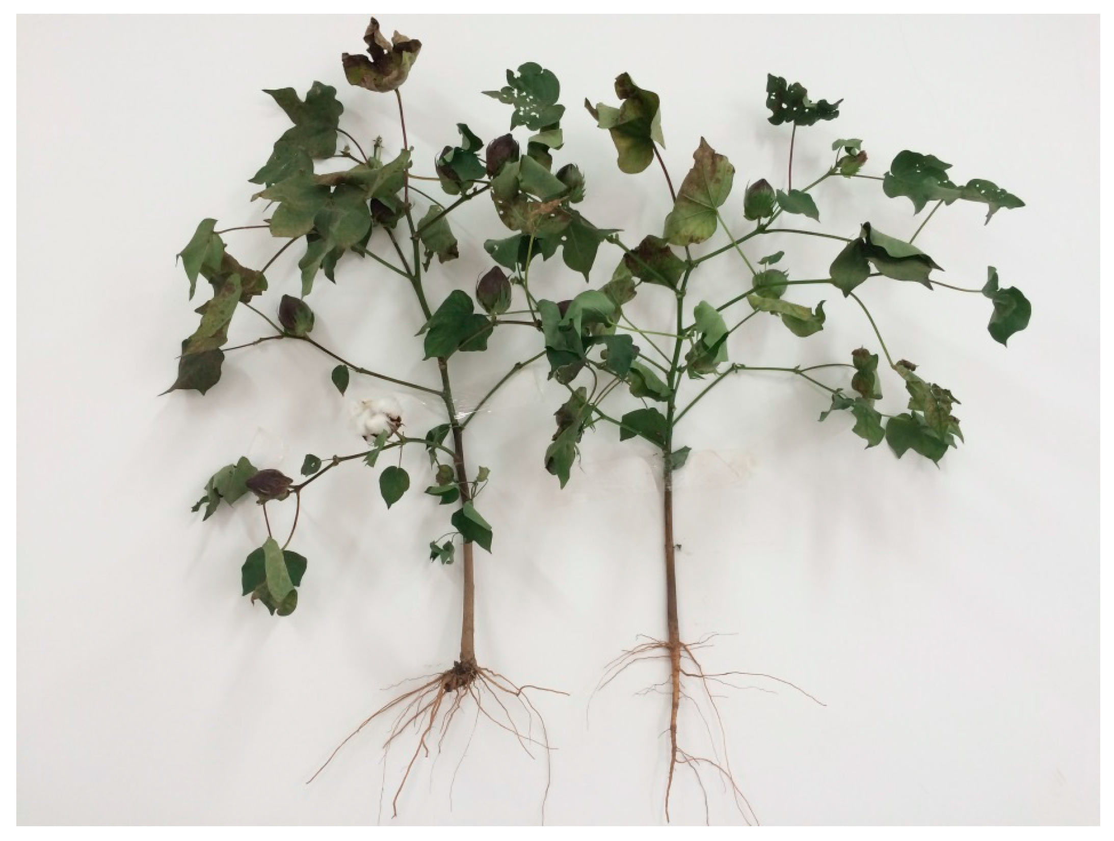
Figure 2.
Irrigation, precipitation and ET0 during the experimental seasons from 2013 to 2015. Abbreviations: BI, border irrigation; and SDI, surface drip irrigation.
Figure 2.
Irrigation, precipitation and ET0 during the experimental seasons from 2013 to 2015. Abbreviations: BI, border irrigation; and SDI, surface drip irrigation.

Figure 3.
Layout of experimental plots (Unit: m).
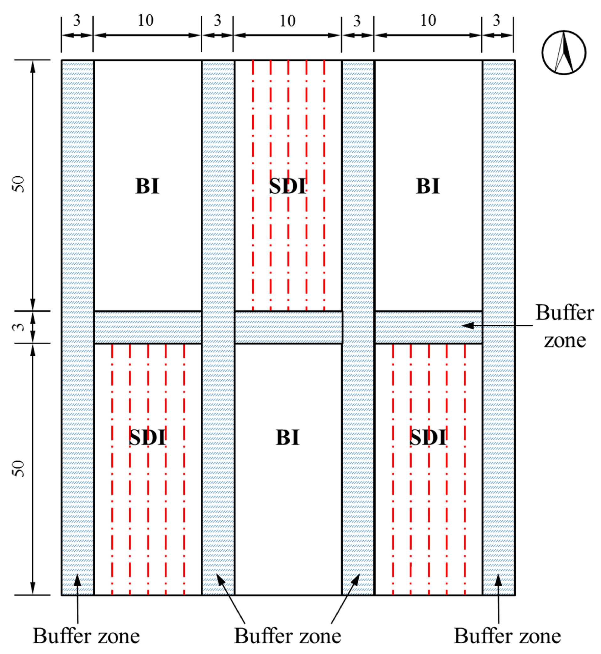
Figure 4.
Schematic representation of the soil core method.

Figure 5.
Domain geometry, grid size and boundary conditions used in the HYDRUS-2D model under different irrigation methods. Abbreviations: BI, border irrigation; and SDI, surface drip irrigation.
Figure 5.
Domain geometry, grid size and boundary conditions used in the HYDRUS-2D model under different irrigation methods. Abbreviations: BI, border irrigation; and SDI, surface drip irrigation.
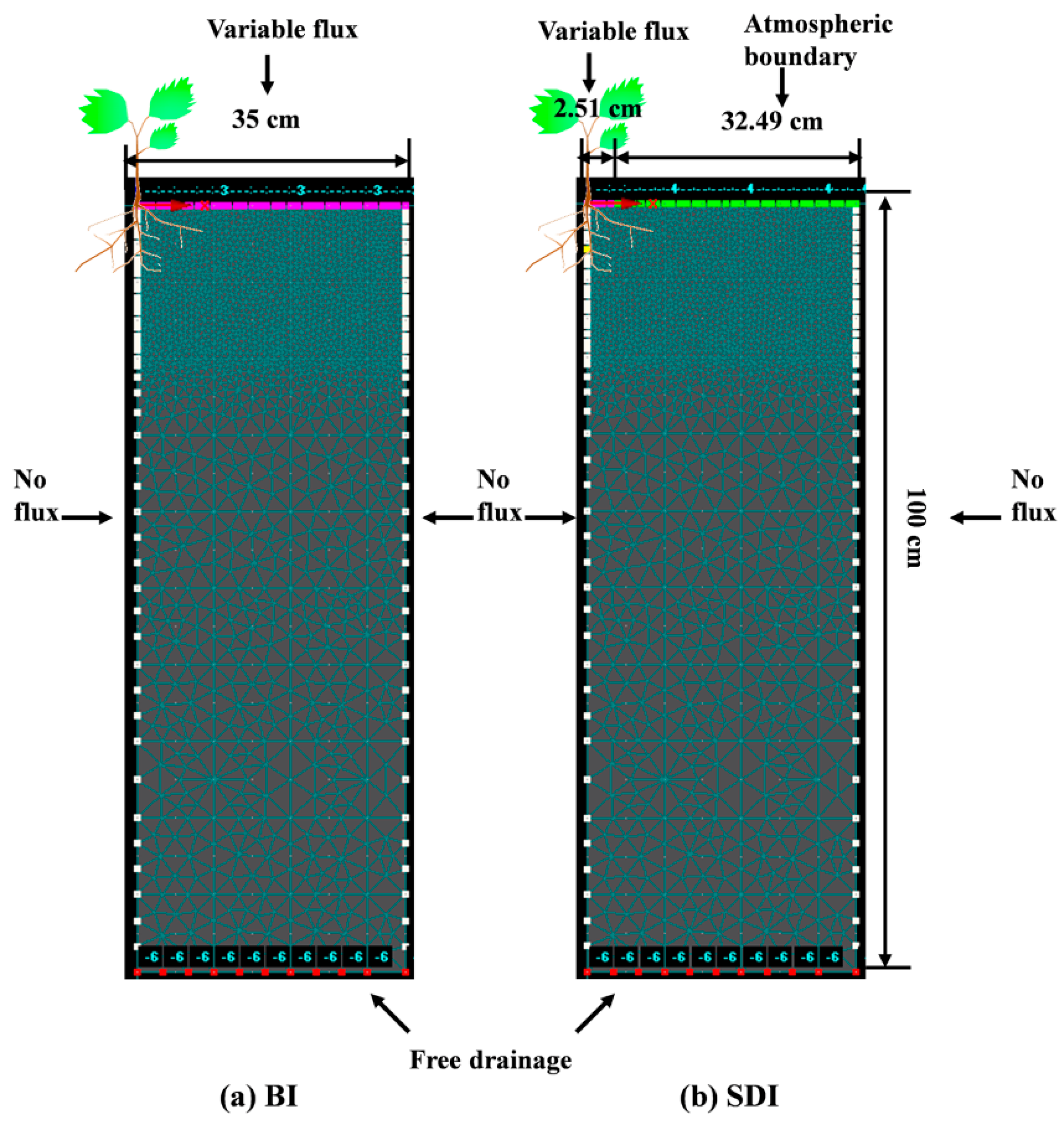
Figure 6.
Two-dimensional RLD of transplanted cotton. Abbreviations: BI, border irrigation; SDI, surface drip irrigation; and RLD, root length density.
Figure 6.
Two-dimensional RLD of transplanted cotton. Abbreviations: BI, border irrigation; SDI, surface drip irrigation; and RLD, root length density.

Figure 7.
Two-dimensional RBD of transplanted cotton. Abbreviations: BI, border irrigation; SDI, surface drip irrigation; and RBD, root biomass density.
Figure 7.
Two-dimensional RBD of transplanted cotton. Abbreviations: BI, border irrigation; SDI, surface drip irrigation; and RBD, root biomass density.

Figure 8.
Variations in the RLD, RSAD, RTND and RD of transplanted cotton in 2014. Abbreviations: BI, border irrigation; SDI, surface drip irrigation; RLD, root length density; RSAD, root surface area density; RTND, root tip number density; and RD, root diameter. The vertical bars represent the standard errors of the means. Different lowercase letters indicate significant differences (p < 5%) between the two treatments.
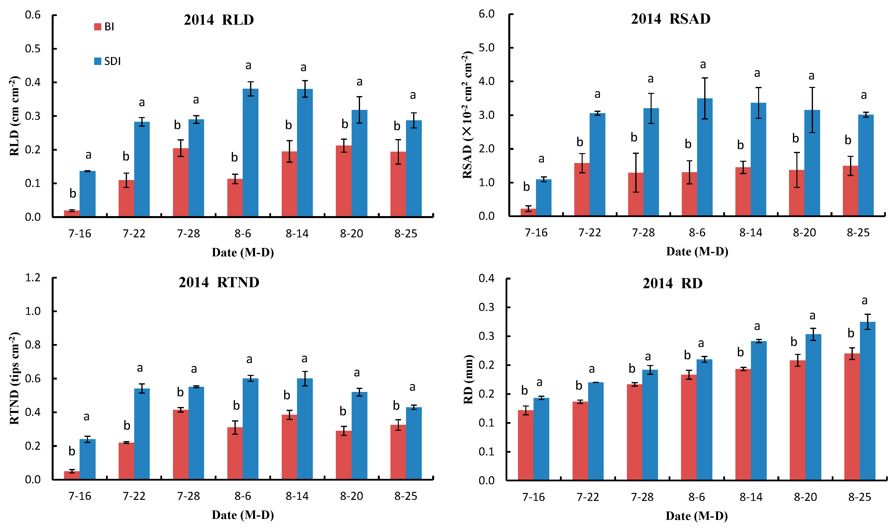
Figure 9.
Variations in the RLD, RSAD, RTND and RD of transplanted cotton in 2015. Abbreviations: BI, border irrigation; SDI, surface drip irrigation; RLD, root length density; RSAD, root surface area density; RTND, root tip number density; and RD, root diameter. The vertical bars represent the standard errors of the means. Different lowercase letters indicate significant differences (p < 5%) between the two treatments.
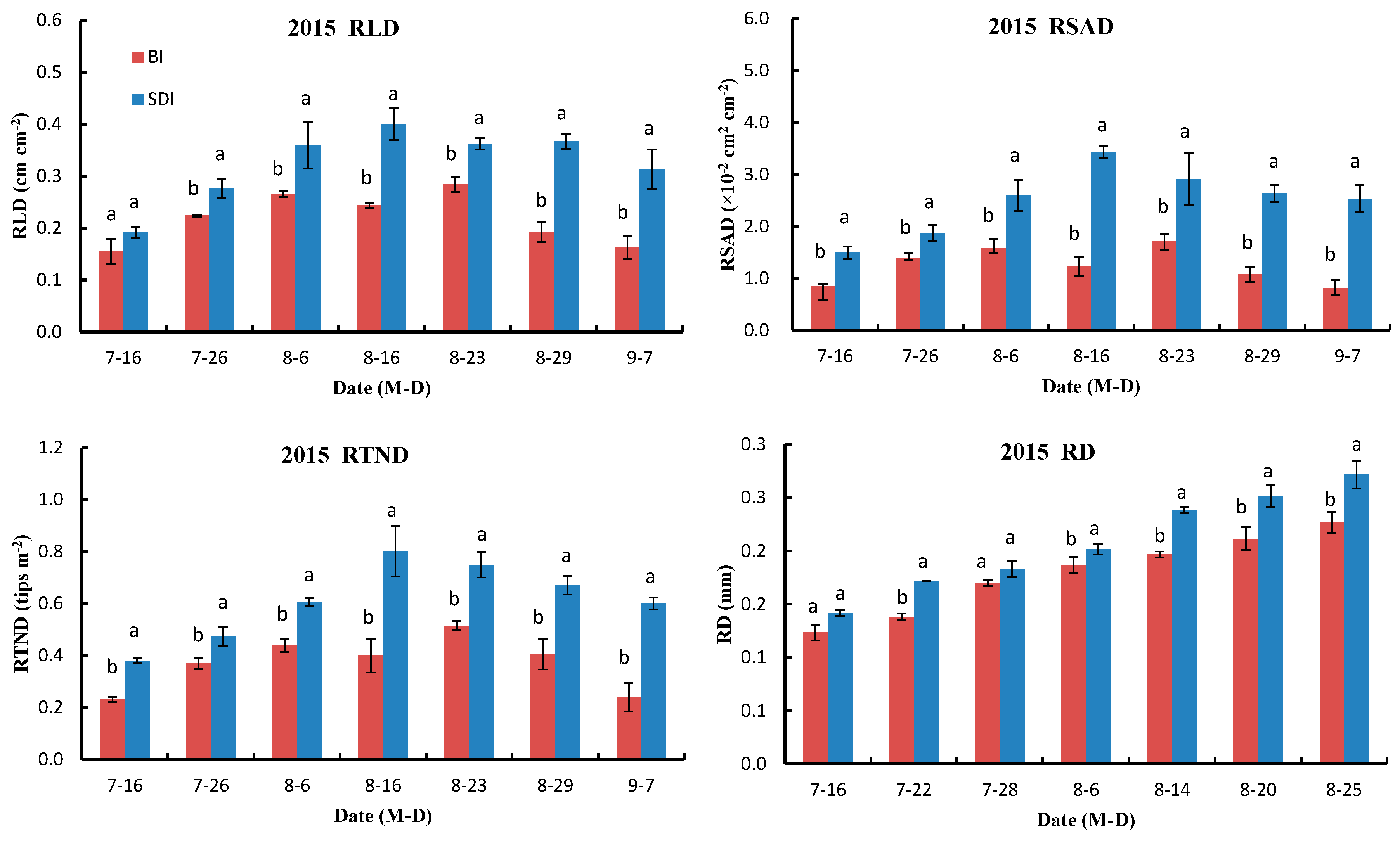
Figure 10.
Comparison of the simulated and observed soil water contents (SWCs) under the two irrigation methods.
Figure 10.
Comparison of the simulated and observed soil water contents (SWCs) under the two irrigation methods.

Figure 11.
Simulated SWCs (lines) and measured SWCs (dots) at various depths in the row of cotton plants in 2013. Abbreviations: BI, border irrigation; SDI, surface drip irrigation; and SWC, soil water content. The vertical bars represent the standard errors of the means.
Figure 11.
Simulated SWCs (lines) and measured SWCs (dots) at various depths in the row of cotton plants in 2013. Abbreviations: BI, border irrigation; SDI, surface drip irrigation; and SWC, soil water content. The vertical bars represent the standard errors of the means.

Figure 12.
Simulated SWCs (lines) and measured SWCs (dots) at various depths in the middle of the inter-rows (0.35 m from the row) of cotton plants in 2013. Abbreviations: BI, border irrigation; SDI, surface drip irrigation; and SWC, soil water content. The vertical bars represent the standard errors of the means.


Table 1.
Soil physical properties in the experimental field.
| Depth (cm) | Soil Texture a | Particle Size Distribution (g 100 g−1) | Bulk Density (Mg m−3) | Field Capacity (cm3 cm−3) | ||
|---|---|---|---|---|---|---|
| <0.002 mm | 0.02–0.002 mm | 2.0–0.02 mm | ||||
| 0–20 | loam | 4 | 43 | 53 | 1.56 | 0.34 |
| 20–40 | silt loam | 7 | 45 | 48 | 1.58 | 0.31 |
| 40–60 | silt loam | 6 | 48 | 46 | 1.54 | 0.33 |
| 60–80 | silt loam | 5 | 47 | 48 | 1.42 | 0.28 |
| 80–100 | sandy loam | 2 | 17 | 81 | 1.45 | 0.29 |
Note: a Soil texture was determined according to the international soil texture classification system.
Table 2.
Agronomic practices during the experiments.
| Practices | 2013 | 2014 | 2015 |
|---|---|---|---|
| Sowing | 11 May | 6 May | 6 May |
| Transplantation | 13 June | 6 June | 10 June |
| Fertilizer application | 13 June 25 June | 6 June 7 July | 10 June 8 July |
| Spraying of pesticides | 15 July 2 August | 30 June 25 July 5 August | 1 July 30 July |
| Hand cutting of plant growth | 30 July | 25 July | 25 July |
| Spraying of mepiquat chloride | 25 July 6 August | 27 July 5 August | 27 July 6 August |
| Pruning | 30 July 13 August | 23 July 6 August | 24 July 7 August |
| Harvest | 4 October 20 October | 26 September 13 October | 27 September 15 October |
Table 3.
Technical parameters of the different irrigation methods. Abbreviations: BI, border irrigation; and SDI, surface drip irrigation.
Table 3.
Technical parameters of the different irrigation methods. Abbreviations: BI, border irrigation; and SDI, surface drip irrigation.
| Irrigation Method | Design Specifications | Field Surface Slope | Irrigation Flow | Equipment Specifications |
|---|---|---|---|---|
| BI | Border width, 2.1 m; border length, 50 m; 3 rows of cotton per plot | 0.002 | Flow per unit width into the furrow, 4 L s−1 m−1 | - |
| SDI | Laying length, 25 m; tube spacing, 0.7 m | - | Emitter flow, 2.0 L h−1 | Inter-tube dripper with 16 mm diameter; emitters 0.2 m apart; working pressure of 0.1 MPa |
Table 4.
Soil hydraulic parameters of the van Genuchten–Mualem model at the experimental site. Saturated water content () and saturated hydraulic conductivity () were measured values, whereas , α and n were estimated through inverse simulation.
Table 4.
Soil hydraulic parameters of the van Genuchten–Mualem model at the experimental site. Saturated water content () and saturated hydraulic conductivity () were measured values, whereas , α and n were estimated through inverse simulation.
| Depth (cm) | (cm3 cm−3) | (cm3 cm−3) | (cm3 Day−1) | n | l | |
|---|---|---|---|---|---|---|
| 0~20 | 0.127 | 0.467 | 27.6 | 0.012 | 1.54 | 0.5 |
| 20~40 | 0.096 | 0.417 | 9.7 | 0.017 | 1.31 | 0.5 |
| 40~60 | 0.095 | 0.424 | 4.7 | 0.022 | 1.21 | 0.5 |
| 60~80 | 0.107 | 0.487 | 12.6 | 0.009 | 1.46 | 0.5 |
| 80~100 | 0.066 | 0.501 | 84.7 | 0.012 | 1.88 | 0.5 |
Table 5.
The RLD (cm cm−3) measured at different soil depths in 2013, 2014 and 2015. Abbreviations: BI, border irrigation; SDI, surface drip irrigation; and RLD, root length density. Letters indicate statistical significance at p = 0.05 level within the same row, and the values are the means of three replicates.
| Soil Depth (cm) | BI | SDI | ||||
|---|---|---|---|---|---|---|
| 2013 | 2014 | 2015 | 2013 | 2014 | 2015 | |
| 0–10 | 0.47 b | 0.30 c | 0.44 bc | 0.67 a | 0.47 b | 0.64 a |
| 10–20 | 0.44 b | 0.31 c | 0.37 bc | 0.58 a | 0.40 b | 0.45 a |
| 20–30 | 0.40 bc | 0.26 d | 0.29 cd | 0.55 a | 0.37 bcd | 0.43 ab |
| 30–40 | 0.34 a | 0.16 b | 0.20 b | 0.38 a | 0.17 b | 0.13 b |
| 40–50 | 0.29 a | 0.14 b | 0.13 b | 0.31 a | 0.07 b | 0.06 b |
| 50–60 | 0.25 a | 0.06 bc | 0.09 b | 0.11 b | 0.01 c | - |
| 60–70 | 0.12 a | - | 0.03 b | - | - | - |
Table 6.
The RBD (mg cm−3) measured at different soil depths in 2013, 2014 and 2015. Abbreviations: BI, border irrigation; SDI, surface drip irrigation; and RBD, root biomass density. Letters indicate statistical significance at p = 0.05 level within the same row and the values are the means of three replicates.
| Soil Depth (cm) | BI | SDI | ||||
|---|---|---|---|---|---|---|
| 2013 | 2014 | 2015 | 2013 | 2014 | 2015 | |
| 0–10 | 0.082 d | 0.108 c | 0.129 c | 0.111 c | 0.191 a | 0.164 b |
| 10–20 | 0.064 cd | 0.056 d | 0.066 bcd | 0.087 b | 0.123 a | 0.079 bc |
| 20–30 | 0.044 a | 0.087 a | 0.038 a | 0.054 a | 0.050 a | 0.065 a |
| 30–40 | 0.037 a | 0.023 ab | 0.028ab | 0.036 a | 0.024 ab | 0.021 b |
| 40–50 | 0.032 a | 0.024 ab | 0.021 bc | 0.024 b | 0.014 c | 0.015 c |
| 50–60 | 0.030 a | 0.026 ab | 0.017 abc | 0.012 bcd | 0.005 cd | - |
| 60–70 | 0.015 a | - | 0.008 b | - | - | - |
Table 7.
Parameters of the two-dimensional model of the root length density (RLD) of transplanted cotton.
Table 7.
Parameters of the two-dimensional model of the root length density (RLD) of transplanted cotton.
| Growth Period | Irrigation Method | px | pz | x* | z* |
|---|---|---|---|---|---|
| Seedling stage | BI | 1.03 | 1.39 | 10 | 12.73 |
| SDI | 0.02 | 0.03 | 5 | 2.12 | |
| Squaring stage | BI | 1.019 | 1.39 | 10 | 17.68 |
| SDI | 0.04 | 0.09 | 5 | 4.95 | |
| Bloom and boll-forming stage | BI | 0.719 | 1.39 | 15 | 21.21 |
| SDI | 0.11 | 0.21 | 5 | 5.66 | |
| Boll opening stage | BI | 1.019 | 1.59 | 15 | 24.04 |
| SDI | 0.22 | 0.35 | 5 | 6.36 |
© 2017 by the authors. Licensee MDPI, Basel, Switzerland. This article is an open access article distributed under the terms and conditions of the Creative Commons Attribution (CC BY) license (http://creativecommons.org/licenses/by/4.0/).
Share and Cite
MDPI and ACS Style
Zhang, H.; Liu, H.; Sun, C.; Gao, Y.; Gong, X.; Sun, J.; Wang, W. Root Development of Transplanted Cotton and Simulation of Soil Water Movement under Different Irrigation Methods. Water 2017, 9, 503. https://doi.org/10.3390/w9070503
AMA Style
Zhang H, Liu H, Sun C, Gao Y, Gong X, Sun J, Wang W. Root Development of Transplanted Cotton and Simulation of Soil Water Movement under Different Irrigation Methods. Water. 2017; 9(7):503. https://doi.org/10.3390/w9070503
Chicago/Turabian StyleZhang, Hao, Hao Liu, Chitao Sun, Yang Gao, Xuewen Gong, Jingsheng Sun, and Wanning Wang. 2017. "Root Development of Transplanted Cotton and Simulation of Soil Water Movement under Different Irrigation Methods" Water 9, no. 7: 503. https://doi.org/10.3390/w9070503
Note that from the first issue of 2016, this journal uses article numbers instead of page numbers. See further details here.