A Hybrid Model for Forecasting Groundwater Levels Based on Fuzzy C-Mean Clustering and Singular Spectrum Analysis


1
University of Belgrade-Faculty of Mining and Geology, Đušina 7, 11000 Belgrade, Serbia
2
Čedomir Cvijović, Department of Geodesy, Belgrade University College of Applied Studies in Civil Engineering and Geodesy, Hajduk Stanka 2, 11000 Belgrade, Serbia
*
Author to whom correspondence should be addressed.
Water 2017, 9(7), 541; https://doi.org/10.3390/w9070541
Submission received: 27 April 2017
/
Revised: 11 July 2017
/
Accepted: 15 July 2017
/
Published: 19 July 2017
(This article belongs to the Special Issue Modeling of Water Systems)
Abstract
:Having the ability to forecast groundwater levels is very significant because of their vital role in basic functions related to efficiency and the sustainability of water supplies. The uncertainty which dominates our understanding of the functioning of water supply systems is of great significance and arises as a consequence of the time-unbalanced water consumption rate and the deterioration of the recharge conditions of captured aquifers. The aim of this paper is to present a hybrid model based on fuzzy C-mean clustering and singular spectrum analysis to forecast the weekly values of the groundwater level of a groundwater source. This hybrid model demonstrates how the fuzzy C-mean can be used to transform the sequence of the observed data into a sequence of fuzzy states, serving as a basis for the forecasting of future states by singular spectrum analysis. In this way, the forecasting efficiency is improved, because we predict the interval rather than the crisp value where the level will be. It gives much more flexibility to the engineers when managing and planning sustainable water supplies. A model is tested by using the observed weekly time series of the groundwater source, located near the town of Čačak in south-western Serbia.
1. Introduction
Maintaining the stability of groundwater exploitation represents a key issue in attaining efficient and sustainable water supplies. It involves stable recharge conditions for the captured aquifer during the exploitation, absence or the slight degradation of the initial seepage characteristics of the aquifer, as well as the selection of an appropriate exploitation regime. An optimal-yield exploitation over a period of many years produces effects related to the spread of general drawdown. It occurs as a consequence of the exploitation regime of all of the intake objects. The fluctuation of the drawdown values is influenced by seasonal wavering in the values of balance elements participating in the recharge of the captured aquifer and the exploitation regime caused by changes of consumption rate.
The deterioration of the recharge conditions of the captured aquifer and its overexploitation lead to an increase in the values of the drawdown and the effective groundwater source radius [1]. For the purpose of the effective management of the exploitation, it is necessary to know the data regarding the drawdown of the groundwater source, independent of the conditions influencing the wavering of drawdown values. In this way, we can define the range of possible total flow of the groundwater source, primarily in dry season periods.
Many models and techniques have been proposed to forecast time series in hydrogeology: the nonlinear optimization technique, the multiple linear regression method, the hybrid soft-computing technique, the hybrid wavelet packet-support vector regression method, artificial neural-network techniques, the adaptive neuro-fuzzy inference system method, and hydrodynamic modeling [2,3,4,5,6,7]. The singular spectrum analysis was used in this paper but is also implemented by various other authors [8,9,10,11,12,13,14,15,16,17].
City water consumption represents a highly dynamic temporal appearance, which causes great difficulties in the water supply management system. Reliable groundwater level forecasting is broadly recognized for its key role in the efficient management of water resources and consumption. In this paper, we proposed a hybrid model that could effectively forecast groundwater levels and improve the efficiency of the process of their management. The hybrid model combined the fuzzy C-mean clustering algorithm (FCM) and singular spectrum analysis (SSA). The FCM is able to effectively classify the monitored data into temporal states of the groundwater level. In this way, the behavior of the observed system can be defined much more flexibly. The SSA is able to effectively forecast the state of the groundwater level and provide opportunities to make different combinations within the obtained components of the data series. The proposed methodology represents an easier way of modelling groundwater levels and offers an opportunity to describe the behavior of a groundwater source without including the physical characteristics of the location. Furthermore, it can be easily updated with new information. There is an opportunity to transform this one single time series model into a multi-dimensional model by adding another observed parameter; in which case, we can use a multivariate singular spectrum analysis.
The development of the model is related to the forecasting of the future states of the groundwater level (the general drawdown) using data obtained during the period of exploitation. The model is composed of two stages: in the first stage, we make fuzzy states of the monitored data, while in the second, we forecast the future states. By using a fuzzy C-mean clustering algorithm, the original time series is divided into an adequate number of fuzzy states. Accordingly, we can create the adequate fuzzy time series. In many cases, the creation of fuzzy relations among fuzzy time series is a very difficult task. In order to avoid this, we represent fuzzy time series by cluster time series, where each cluster is defined by its center, minimum and maximum value. This approach enables us to apply a deterministic forecasting model based on the singular spectrum analysis. This analysis reveals the structure of the time series, i.e., components such as trend, oscillations and noise. Planners can create different scenarios using different combinations of components. This model is very beneficial to city authorities due to its effective water resource management.
2. Forecasting Model
In this paper, we study the forecasting time of the invariant fuzzy time series of groundwater levels. The fuzzy C-mean algorithm is used for the fuzzification of the observed data, while the SSA is applied to make a forecasting model.
By applying linear recurrent formulae, we predict the future values of cluster centers. After that, the sequence of the forecasted cluster centers is transformed into a sequence of the actual centers obtained by fuzzy C-mean clustering. The transformation uses the equation of the fuzzy C-mean clustering algorithm, which calculates the membership degree. Finally, the developed model produces the interval time series, characterized by the minimum and maximum value of the groundwater level for every point in the future.
The developed model was tested by using the real data obtained by monitoring the groundwater source Perminac. It is located in the upstream area of Čačak city. The groundwater source contains 14 wells with a maximum total capacity of 131 l/s and an average of 90 l/s. In recent years, overexploitation caused a significant decrease in the groundwater level in the wider area of the groundwater source. Accordingly, some wells were excluded from the exploitation, and supply restrictions were introduced as a way of stabilizing consumption during the summer months.
2.1. Fuzzy Time Series
“Let be the universe of observed data on which fuzzy sets are defined and let be a collection of . Then, is called a fuzzy time series on .”
Song and Chissom [18] defined fuzzy relations among fuzzy time series, which are based on the assumption that the values of fuzzy time series are fuzzy sets, and the observation of time t is caused by the observations of the previous times [19].
If for any , there exist and a fuzzy relation such that , where ”” is the relation, then is said to be caused by only. It is expressed as follows:
Suppose that is caused by only, or by or or . This relation can be expressed as follows:
Equation (2) represents the first-order model of . If is caused by
simultaneously, then their relations are represented as:
Equation (3) represents the k-th order model of , and is a relation matrix describing the fuzzy relationship between and .
To fuzzify the observed data, we apply the fuzzy C-mean algorithm.
2.2. A Brief Description of the Fuzzy C-mean Algorithm
In order to divide the observed data into an adequate number of fuzzy states, we apply the fuzzy C-mean clustering algorithm [20,21,22,23] over the set . The reason that we clustered the time series is primarily related to the need to develop models that use the results of monitoring in a form that represents the states of the observed appearance. Decision-making models based on the interval inputs are much more flexible than deterministic models. Management models have a much higher confidence because they incorporate uncertainties expressed by intervals into management systems.
The fuzzy C-mean algorithm is a method based on the minimization of a generalized least-squared errors-function. Given a set , where N is the number of the observed data and q is the dimension of the sample . Every cluster is a fuzzy set defined by the relative closeness of space S. Suppose that there is a groundwater level vector composed of M cluster centers; . For the i-th relative closeness and m-th cluster center, there is a membership degree indicating with what degree the relative closeness SN belongs to the cluster center vector Cm, which results in a fuzzy partition matrix .
Let uim be the membership, cm the center of the cluster, N the number of observed data and M the number of clusters. This algorithm aims to determine cluster centers and the fuzzy partition matrix by minimizing the following function:
subject to
where dim is Euclidean distance between the observation and the center of the cluster, defined as:
Finally, the objective function is:
The objective function J represents the intra-cluster variance. If we want to have those elements that are most similar to the cluster center in a given cluster, we can do this by minimizing the variance inside the cluster. The exponent ω is used to adjust the weighting effect of membership values. A large ω will increase the fuzziness of the function J. Pal and Bezdek [24] suggested that ω in the interval [1.5, 2.5] was generally recommended for use in FCM.
In this paper, the value of ω is set to 2 as a midpoint of the suggested interval. The objective function is iteratively minimized. In j-th iteration, the values of and are updated as follows:
The iteration process stops at , where represents the minimum amount of improvement. Sorting the sequence of obtained centers in an ascending order gives us .
The fuzzification of the data is done according to the results of the final fuzzy partition matrix.
The number of fuzzy sets corresponds to the number of clusters. Each row of the matrix U represents the fuzzy state of that observation. Accordingly, we obtain the fuzzy state matrix of the observed data:
The state of the observed data is defined as:
Finally, the sequence Aim represents a fuzzy time series on . In this way, we obtain the transitions from one state to another over the time of observation; .
The creation of a set of certain transition rules for fuzzy relationships between states can be very difficult. To overcome this situation, we transform the fuzzy time series into an adequate time series of the center of the clusters. This approach enables us to apply a deterministic forecasting model based on the singular spectrum analysis.
2.3. Forecasting Model Based on the Singular Spectrum Analysis
The process of the transformation of the fuzzy time series into a crisp time series is based on the fact that each fuzzy state can be represented by a corresponding center of the cluster. Accordingly, the following time series, , are obtained.
The forecasting algorithm is based on SSA methodology [25,26,27]. In SSA terminology, it is often assumed that the series is noisy with an arbitrary series length N. The SSA technique consists of two main complementary stages: decomposition and reconstruction. The noisy series is decomposed in the first stage, and the noisy reduced series is reconstructed at the second stage. The reconstructed series will be used for forecasting the future values.
Consider the stochastic process and suppose that a realization of size N from this process is available: . Since we are faced with time-invariant series, and for simplicity, we can rewrite the realization as follows: .
The first stage of the algorithm, called decomposition, includes the following two steps: embedding and singular value decomposition (SVD).
Embedding is a mapping that transfers a one-dimensional time series of centers into a multidimensional matrix with vectors , where is the window length and . The window length represents a vector of L observations of the original series. If we remember Equation (3), we can see the window length model is similar to the k-th order model of the fuzzy time series, but taking into account original values from t = 1 to t = L. The usual value of L is (N + 1)/2 if N is odd and N/2 or (N/2) + 1 if N is even (for more details see [27]). The result of this step is the trajectory matrix:
The trajectory matrix Y is the Hankel matrix where all elements along the diagonal i + j = const are equal.
The SVD of matrix Y is based on the spectral decomposition of the lag-covariance matrix . Denote as the eigenvalues of , arranged in decreasing order , and the corresponding eigenvectors. The SVD of the trajectory matrix Y can be represented as
where d is the rank of Y.
The second stage of the algorithm, called reconstruction, includes the following two steps: grouping and diagonal averaging or Hankelization.
The grouping step corresponds to the splitting of the set of matrices into several disjointed subsets and the summing of the matrices within each subset. The procedure of choosing the subsets is called grouping. As a simple case, where we have only signal and noise components (k = 2), we use two subsets, and , and associate the subset with the signal component and the subset with noise. Selecting the appropriate number of eigenvalues (r) to be included into the reconstruction is very important. If we take an r smaller than it should really be, some parts of the signal will be lost and the accuracy of the reconstructed series will be lower. On the other hand, if the value of r is too large, then a lot of noise will be included into the reconstructed series. After performing a singular value decomposition of the trajectory matrix, singular values ordered in a decreasing manner are obtained. The plot of the logarithms of the obtained singular values gives very useful information regarding breaks in the eigenvalue spectra. The component where a significant drop in values occurs can be interpreted as the start of the noise floor [28].
Diagonal averaging or Hankelization represents the last step in SSA, where each reconstructed trajectory matrix (see Equation (16)) is transformed into a new one-dimensional time series of length N. This corresponds to the averaging of the matrix elements over the anti-diagonals i + j=k + 1; the selection k = 1 gives , for k = 2, , and so on. For example, the reconstructed trajectory matrix is transformed into a new one-dimensional time series . Finally, the original time series CN is decomposed into a sum of r vectors or principal components:
The reconstructed (extracted) series will be used to forecast new data points.
The third stage of the algorithm concerns the future states of the groundwater level and is based on the linear recurrent formulae. Let denote the vector of the first L-1 coordinates of the eigenvectors and indicate the last coordinate of the eigenvectors . Define the verticality coefficient as
If , then the h-step ahead SSA forecasting exists. Obviously, the value of r must be carefully selected to satisfy the previous inequality, as well as to separate the signal from the noise components. The main concept behind the definition of the value of r is related to the dependence between the different reconstructed (principal) components [28]. The weighted correlation represents the level of dependence between the two series and :
where
- —absolute value of the weighted Frobenius inner product,
- —the weighted norm
- —vector of weights.
If the two reconstructed components have zero w-correlation, it means that these two components are well separated. Large values of w-correlations between the reconstructed components indicate that the components should possibly be gathered into one group and correspond to the same component in SSA decomposition [28]. The obtained correlations can be effectively represented by the grey-scaled correlation matrix.
The linear vector of coefficients is calculated as follows:
The h-step ahead SSA forecasting is achieved by the following equation:
where
The accuracy of the proposed model is estimated by the mean absolute percentage error (MAPE) and the coefficient of determination (R2):
where s(t) is the actual value, is the forecasted value of the cluster center and is the average of the observed set. R2 is a positive number which demonstrates how well the model fits the data. It can take values between zero and one, where zero indicates that there is a poor correlation between the model output and the actual data. Note, there is a difference between the actual and the forecasted value of the cluster center. The sequence of the forecasted cluster centers is now transformed into a sequence of the actual centers by Equation (11); .
According to the concept of the C-mean clustering algorithm, each fuzzy state can be defined as a triplet; , where is equal to the element of the cluster with the minimum value, is equal to the element with the maximum value and has already been explained. Finally, the developed model produces the interval time series .
3. Numerical Example
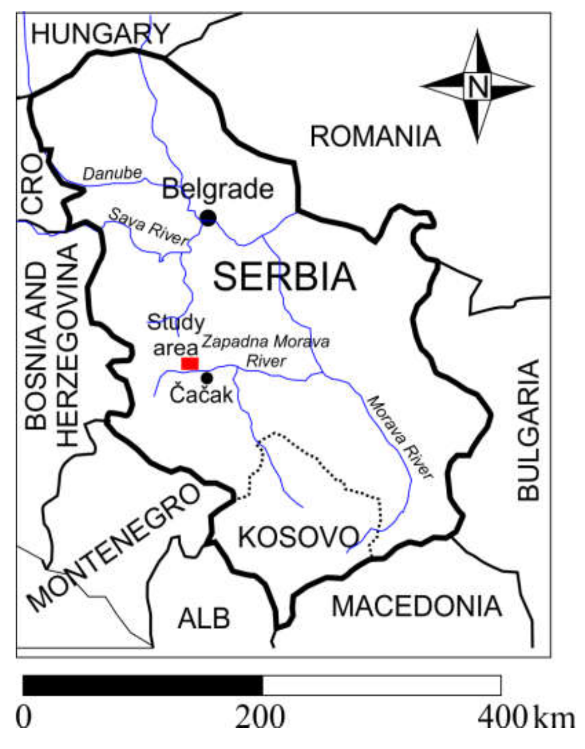
The groundwater source of Perminac was formed in the alluvion of the Zapadna Morava river, in the Zapadna Morava valley in the south-western region of the Republic of Serbia. Alluvial sediments are composed of sand and gravel varying from 4 to 6 m in thickness. The presence of a hydraulic connection to the Zapadna Morava river enables the intensive recharge of the aquifer. The groundwater source was formed along the left bank of the river, upstream from the town of Čačak. The location of the study area is represented by Figure 1.
The data used in this paper includes weekly groundwater level time series. We divided the set of data into the training subset, where the model is applied, and the validation subset, where the comparison between the forecasted and actual values is made. About 85% of the data was used to check the confidence of the model, while about 15% was used to check its validity. The main reason for such data division was primarily influenced by a lack of funds for a longer period of exploration; the monitoring lasted only one year. By using this method of data division, we wanted to be sure about the confidence of the model. Usually, 2/3 of data is used for training and 1/3 for validation.
The observed data is represented in Table 1.
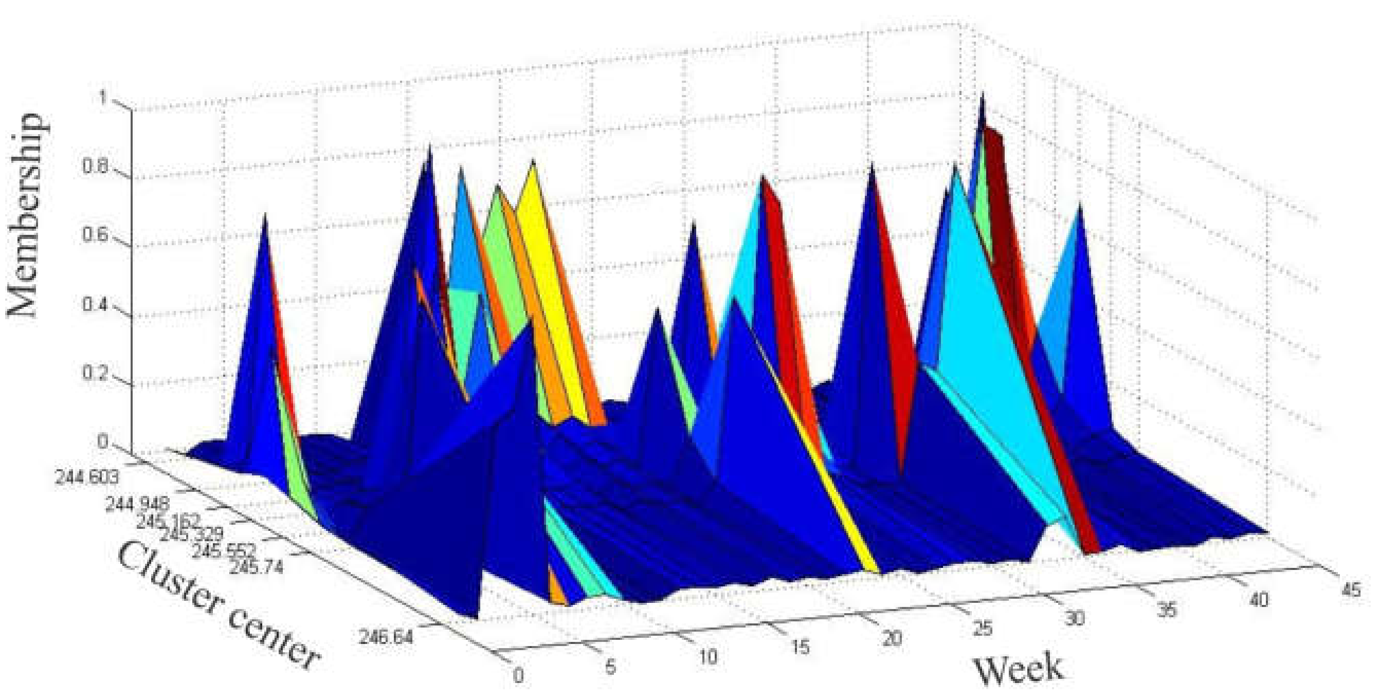
We used the exponent ω = 2 and seven clusters to partition the original time series (from week 1 to 45) and the resulting cluster centroids were as follows: C={c1,c2,c3,c4,c5,c6,c7}={244.603;244.994;245.162;245.329;245.552;245.740;246.641}. Next, the historical data was fuzzified with respect to where the maximum membership degree occurred. For example, the fuzzy state for week 7 was A5 because c5 had the greatest membership degree. Table 2 and Figure 2 and Figure 3 give the results of the fuzzification of the data based on the application of the fuzzy C-mean clustering algorithm.
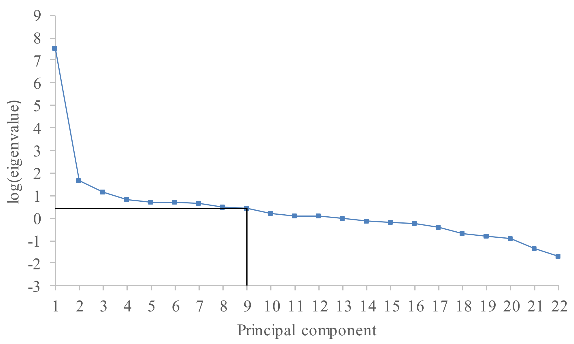
Having obtained the sequence of fuzzy state transitions, we can continue searching for the relation which describes it. For that purpose, we have performed an SSA decomposition of the cluster center time series. The window length L in the SSA decomposition has taken a value of 23, while the value of K was also 23. The initial cluster of the center time series was decomposed into 22 principal components, and they were ordered with respect to the decreasing value of their eigenvalues. Figure 4 depicts the plot of the logarithms of the 22 singular values. Here, a significant drop in the logarithm values occurs around component 9, and we adopted this as the start point of the noise floor.
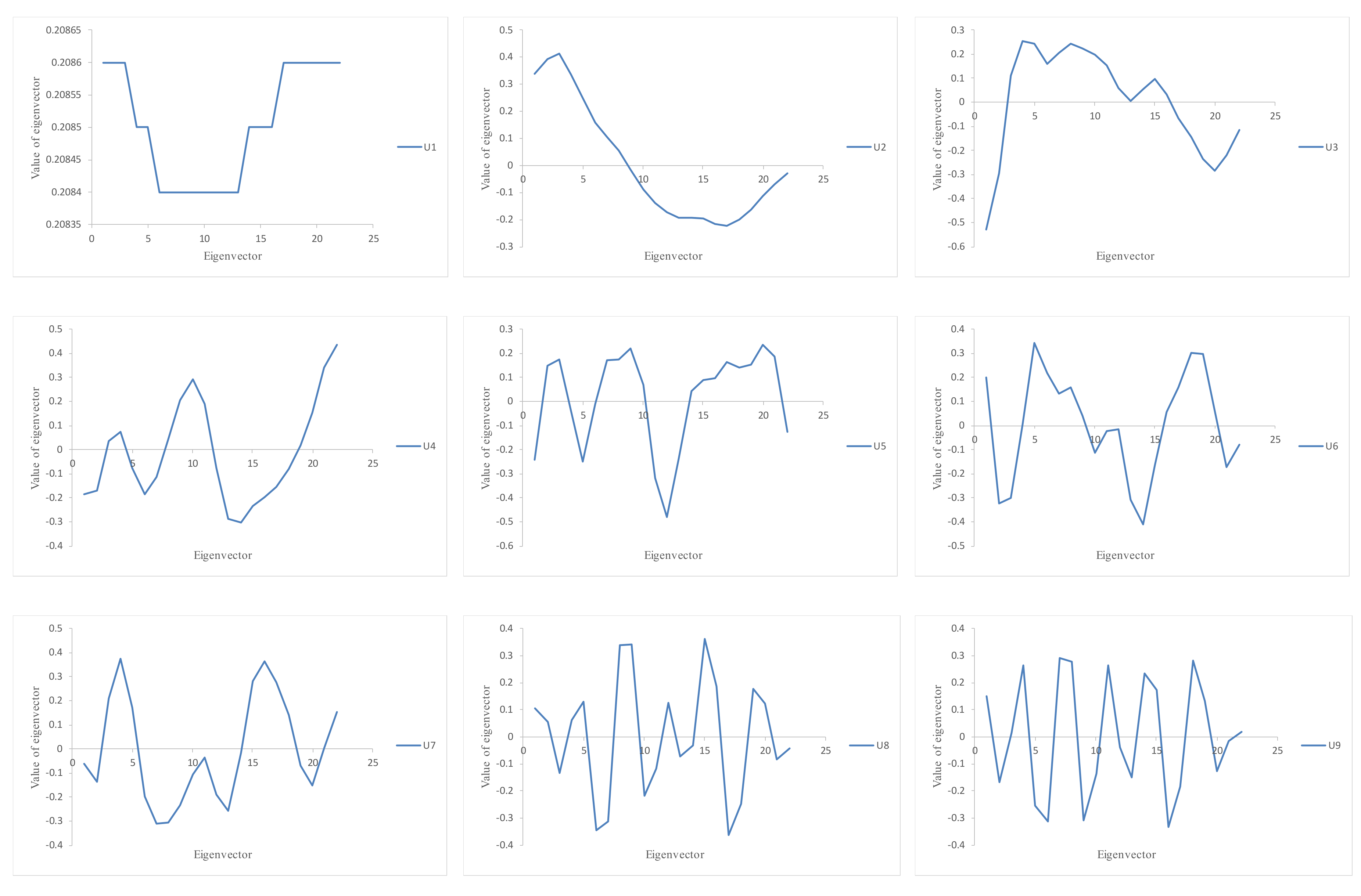
Figure 5 represents the eigenvectors related to the first nine eigenvalues.
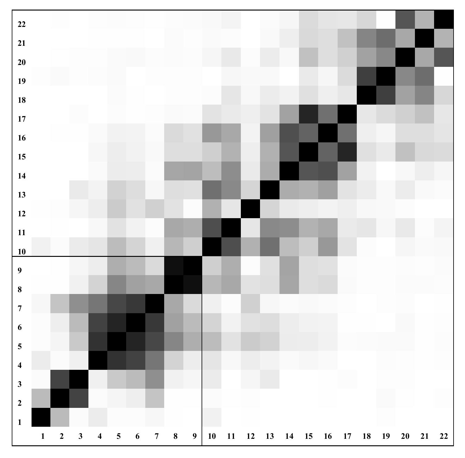
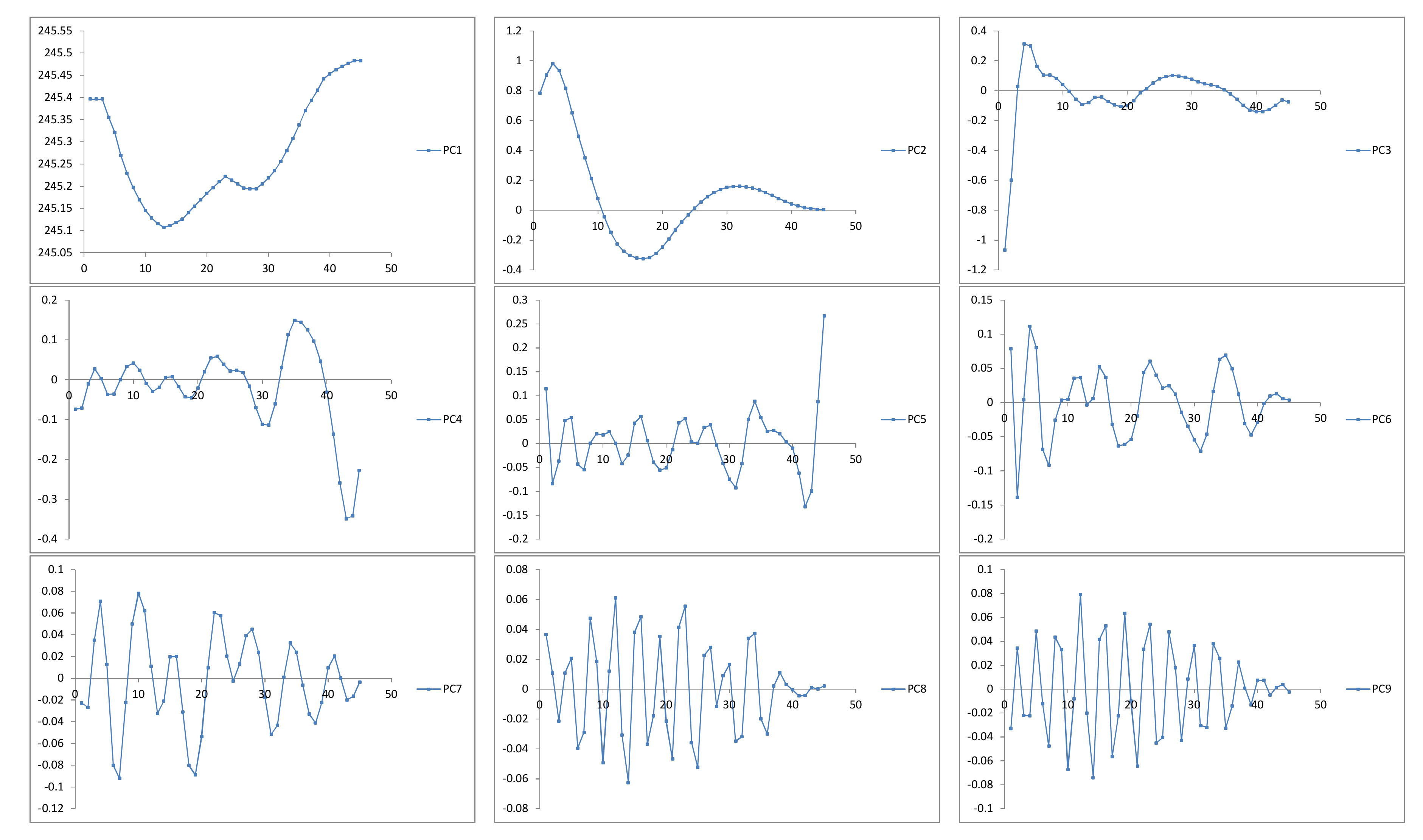
A matrix of weighted grey-scaled correlations between the 22 principal components is represented by Figure 6. The first nine principal components were selected for the reconstruction stage (see Figure 7).
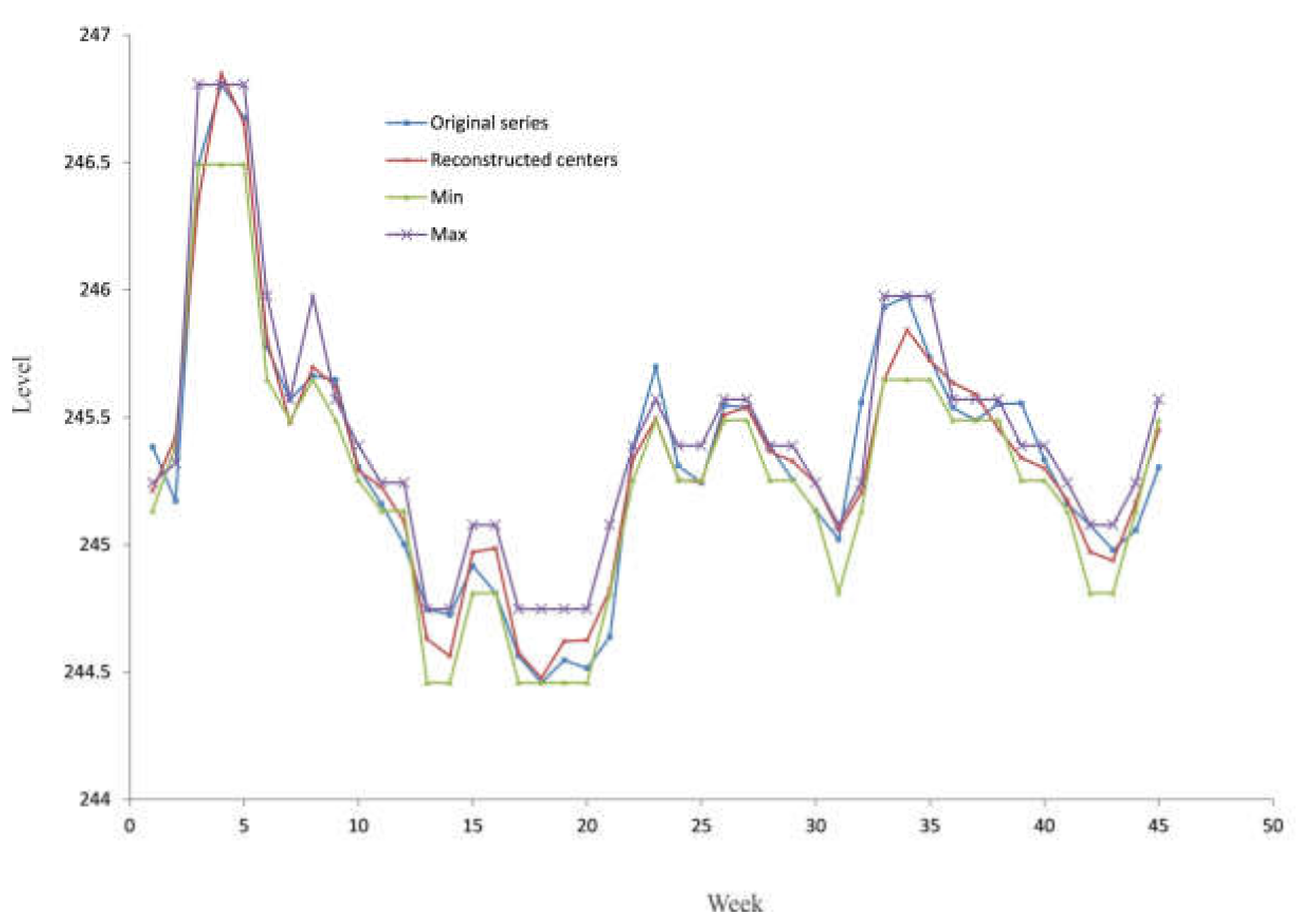
The reconstruction of the original time series CN = 45 using the first nine principal components (r = 9) is represented by Table 3 and Figure 8.
Bold letters indicate the difference between the original and reconstructed fuzzy state for the training subset of data (weeks 1–45). In ten cases, the model missed the original fuzzy state within a range of ±1 state, while the difference was ±2 states in only one case.
The accuracy of the proposed model is estimated by Equations (23) and (24) and represented by Table 4.
The results represented in Table 4 indicate that the model has a very high accuracy and can be used for the forecasting of future states. We used Equation (21) over the period t = 46, 47,…, 52 for the purpose of measuring the validity of the developed model; the results are represented in Table 5.
Bold letters indicate the difference between the original and forecasted fuzzy state for the validation subset of data (weeks 46–52). Only in two cases did the model miss the original fuzzy state within a range of ±1 state. The accuracy of the model for the period of validation is represented by Table 6.
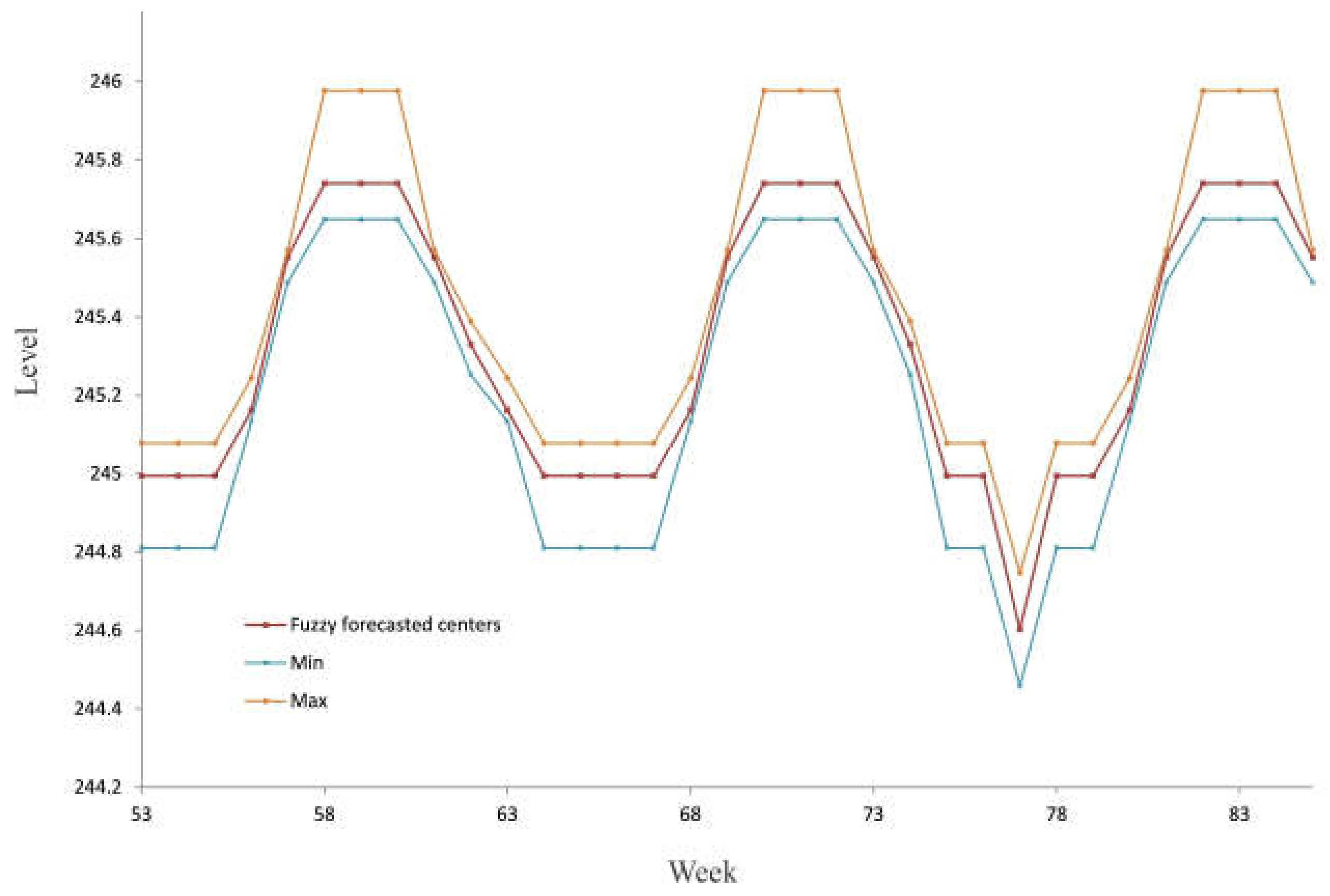
When applying Equation (21), we forecasted the future values of the groundwater level for t = 53, 54,…, 85 (see Figure 9).
4. Conclusions
Having the ability to forecast the future states of any system plays a key role in the planning process. The main aim of this paper was to develop a forecasting model for future states of the groundwater level (the general drawdown) using data obtained during the period of exploitation.
The model is composed of two stages. In the first stage, we make fuzzy states of the monitored data, while in the second, we forecast future states. Using a fuzzy C-mean clustering algorithm, the original time series is divided into an adequate number of fuzzy states. After that, an adequate number of fuzzy time series are created. In many cases, creating the fuzzy relations among the fuzzy time series is a very difficult task. In order to avoid this, the fuzzy time series is represented by an adequate cluster of time series, where each cluster is defined by its center, minimum and maximum value. This approach enables us to apply a deterministic forecasting model based on a singular spectrum analysis.
The validation of the developed hybrid model has been performed using real data obtained by monitoring the groundwater level. The values of the mean absolute percentage error and the coefficient of determination show the high accuracy of the developed model. There are no limits on the application of the model for representing only numerical examples. We can use it to forecast the future states of any time series in hydrogeology. For example, to forecast precipitation, the yield of a groundwater source, and the inflow or outflow of a defined area using different time spans (day, week, month, year).
The forecasted states of the flow or groundwater level that can be obtained by the application of this model enable us to set up state boundary conditions for water supply planners more efficiently. Further research will be focused on the creation of the multivariable forecasting model.
Acknowledgments
Our gratitude goes to the Ministry of Education, Science and Technological Development of the Republic of Serbia for financing projects “OI176022”, “TR33039” and “III43004”.
Author Contributions
All authors contributed to the finalization of paper by joint efforts: D.P. designed the methodology and wrote the final manuscript with Z.G. and D.B. Research plan, fieldwork and initial data analysis was conducted by Č.C.
Conflicts of Interest
The authors declare no conflict of interest.
References
- Bear, J. Hydraulics of Groundwater; McGraw-Hill: New York, NY, USA, 1979. [Google Scholar]
- He, B.; Takase, K.; Wang, Y. Regional groundwater prediction model using automatic parameter calibration SCE method for a coastal plain of Seto Inland Sea. Water Resour. Manag. 2007, 21, 947–959. [Google Scholar] [CrossRef]
- Chang, F.; Chang, L.; Huang, C.; Kao, I. Prediction of monthly regional groundwater levels through hybrid soft-computing techniques. J. Hydrol. 2016, 541, 965–976. [Google Scholar] [CrossRef]
- Raghavendra, S.; Deka, P.C. Forecasting monthly groundwater level fluctuations in coastal aquifers using hybrid Wavelet packet-Support vector regression. Cogent Eng. 2005. [Google Scholar] [CrossRef]
- Emamgholizadeh, S.; Moslemi, K.; Karami, G. Prediction the Groundwater Level of Bastam Plain (Iran) by Artificial Neural Network (ANN) and Adaptive Neuro-Fuzzy Inference System (ANFIS). Water Resour. Manag. 2014, 28, 5433–5446. [Google Scholar] [CrossRef]
- Sahoo, S.; Madan, K.J. Groundwater-level prediction using multiple linear regression and artificial neural network techniques: A comparative assessment. Hydrogeol. J. 2013, 21, 1865–1887. [Google Scholar] [CrossRef]
- Polomčić, D.; Bajić, D. Application of Groundwater modeling for designing a dewatering system: Case study of the Buvač Open Cast Mine, Bosnia and Herzegovina. Geol. Croat. 2015, 68, 123–137. [Google Scholar] [CrossRef]
- Barco, J.; Hogue, T.S.; Girotto, M.; Kendall, D.R.; Putti, M. Climate signal propagation in southern California aquifers. Water Resour. Res. 2010. [Google Scholar] [CrossRef]
- Cao, G.; Zheng, C. Signals of short-term climatic periodicities detected in the groundwater of North China Plain. Hydrol. Process. 2015, 30, 515–533. [Google Scholar] [CrossRef]
- Dickinson, J.E.; Hanson, R.T.; Ferré, T.P.A.; Leake, S.A. Inferring time-varying recharge from inverse analysis of long-term water levels. Water Resour. Res. 2004. [Google Scholar] [CrossRef]
- James, S.C.; Doherty, J.E.; Eddebbarh, A. Practical Postcalibration Uncertainty Analysis: Yucca Mountain, Nevada. Groundwater 2009, 47, 851–869. [Google Scholar] [CrossRef] [PubMed]
- Markovic, D.; Koch, M. Stream response to precipitation variability: A spectral view based on analysis and modelling of hydrological cycle components. Hydrol. Process. 2014, 29, 1806–1816. [Google Scholar] [CrossRef]
- Masbruch, M.D.; Rumsey, C.A.; Gangopadhyay, S.; Susong, D.D.; Pruitt, T. Analyses of infrequent (quasi-decadal) large groundwater recharge events in the northern Great Basin: Their importance for groundwater availability, use, and management. Water Resour. Res. 2016, 52, 7819–7836. [Google Scholar] [CrossRef]
- Shun, T.; Duffy, C.J. Low-frequency oscillations in precipitation, temperature, and runoff on a west facing mountain front: A hydrogeologic interpretation. Water Resour. Res. 1999, 35, 191–201. [Google Scholar] [CrossRef]
- Tiwari, R.K.; Rajesh, R. Imprint of long-term solar signal in groundwater recharge fluctuation rates from Northwest China. Geophys. Res. Lett. 2014, 41, 3103–3109. [Google Scholar] [CrossRef]
- Yiou, P.; Baert, E.; Loutre, M.F. Spectral analysis of climate data. Surv. Geophys. 1996, 17, 619–663. [Google Scholar] [CrossRef]
- Zhang, Q.; Wang, B.; He, B.; Peng, Y.; Ren, M. Singular Spectrum Analysis and ARIMA Hybrid Model for Annual Runoff Forecasting. Water Resour. Manag. 2011, 25, 2683–2703. [Google Scholar] [CrossRef]
- Song, Q.; Chissom, B.S. Fuzzy time series and its models. Fuzzy Sets Syst. 1993, 54, 269–277. [Google Scholar] [CrossRef]
- Li, S.-T.; Cheng, Y.-C.; Lin, S.-Y. A FCM-based deterministic forecasting model for fuzzy time series. Comput. Math. Appl. 2008, 56, 3052–3063. [Google Scholar] [CrossRef]
- Bezdek, J.C.; Enrlich, R.; Full, W. FCM: The fuzzy c-means clustering algorithm. Comput. Geosci. 1984, 10, 191–203. [Google Scholar] [CrossRef]
- Lu, Y.H.; Ma, T.H.; Yin, C.H.; Xie, X.Y.; Tian, W.; Zhong, S.M. Implementation of the Fuzzy C-Means Clustering Algorithm in Meteorogical Data. Int. J. Database Theory Appl. 2013, 6, 1–18. [Google Scholar] [CrossRef]
- Wang, X.; Wang, Y.; Wang, L. Improving fuzzy c-means clustering based on feature-weight learning. Pattern Recognit. Lett. 2004, 25, 1123–1132. [Google Scholar] [CrossRef]
- Chang, C.T.; Lai, J.Z.C.; Jeng, M.D. A fuzzy K-means clustering algorithm using cluster center displacement. J. Inf. Sci. Eng. 2011, 27, 995–1009. [Google Scholar]
- Pal, N.R.; Bezdek, J.C. On cluster validity for fuzzy c-means model. IEEE Trans. Fuzzy Syst. 1995, 1, 370–379. [Google Scholar] [CrossRef]
- Hassani, H.; Zhigljavsky, A. Singular Spectrum Analysis: Methodology and Application to Economics Data. J. Syst. Sci. Complex. 2009, 22, 372–394. [Google Scholar] [CrossRef]
- Harris, T.J.; Yuan, H. Filtering and frequency interpretations of Singular Spectrum Analysis. Physica D 2010, 239, 1958–1967. [Google Scholar] [CrossRef]
- Hassani, H.; Mahmoudvand, R. Multivariate Singular Spectrum Analysis: A general view and new vector forecasting approach. Int. J. Energy Stat. 2013, 1, 55–83. [Google Scholar] [CrossRef]
- Hassani, H. Singular Spectrum Analysis: Methodology and Comparison. J. Data Sci. 2007, 5, 239–257. [Google Scholar]
Figure 1.
Location of the groundwater source.

Figure 2.
Surface plot of membership functions by a fuzzy C-mean algorithm for the observed data (training subset).
Figure 2.
Surface plot of membership functions by a fuzzy C-mean algorithm for the observed data (training subset).

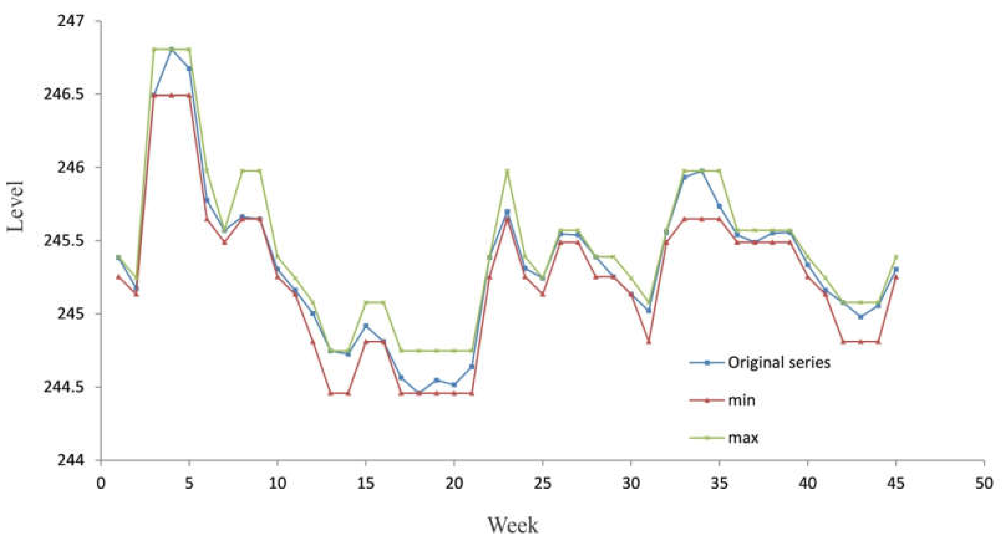
Figure 3.
Interval plot by a fuzzy C-mean algorithm for the observed data (training subset).

Figure 4.
Logarithms of the 22 eigenvalues.

Figure 5.
One-dimensional plots of the first nine eigenvectors.

Figure 6.
The weighted grey-scaled correlation matrix; the white color corresponds to zero values; the black color corresponds to absolute values equal to 1.
Figure 6.
The weighted grey-scaled correlation matrix; the white color corresponds to zero values; the black color corresponds to absolute values equal to 1.

Figure 7.
Principal components obtained by singular spectrum analysis (SSA) decomposition (horizontal axis: week; vertical axis: level).
Figure 7.
Principal components obtained by singular spectrum analysis (SSA) decomposition (horizontal axis: week; vertical axis: level).

Figure 8.
Interval plot by the SSA algorithm for the observed data (training subset).

Figure 9.
Interval plot by the SSA forecasting algorithm.


Table 1.
Historical data of the groundwater level.
| Week | Level | Week | Level | Week | Level | Week | Level |
|---|---|---|---|---|---|---|---|
| 1 | 245.384 | 14 | 244.725 | 27 | 245.539 | 40 | 245.335 |
| 2 | 245.173 | 15 | 244.918 | 28 | 245.389 | 41 | 245.161 |
| 3 | 246.492 | 16 | 244.810 | 29 | 245.253 | 42 | 245.078 |
| 4 | 246.806 | 17 | 244.564 | 30 | 245.134 | 43 | 244.980 |
| 5 | 246.676 | 18 | 244.458 | 31 | 245.021 | 44 | 245.057 |
| 6 | 245.776 | 19 | 244.547 | 32 | 245.559 | 45 | 245.303 |
| 7 | 245.571 | 20 | 244.515 | 33 | 245.932 | 46 | 245.584 |
| 8 | 245.663 | 21 | 244.639 | 34 | 245.977 | 47 | 245.694 |
| 9 | 245.648 | 22 | 245.386 | 35 | 245.735 | 48 | 245.785 |
| 10 | 245.304 | 23 | 245.698 | 36 | 245.539 | 49 | 245.794 |
| 11 | 245.162 | 24 | 245.311 | 37 | 245.489 | 50 | 245.551 |
| 12 | 245.002 | 25 | 245.244 | 38 | 245.552 | 51 | 245.400 |
| 13 | 244.747 | 26 | 245.547 | 39 | 245.556 | 52 | 245.159 |
Note: Bold numbers indicate the validation subset.
Table 2.
Fuzzification of the observed data (training subset).
| Week | Membership Values | Cluster Center | Interval | Fuzzy State | ||||||
|---|---|---|---|---|---|---|---|---|---|---|
| No. | c1 | c2 | c3 | c4 | c5 | c6 | c7 | m | [min;max] | Am |
| 1 | 0.0353 | 0.0708 | 0.1244 | 0.5061 | 0.1638 | 0.0776 | 0.0220 | 245.329 | [245.253;245.389] | A4 |
| 2 | 0.0150 | 0.0480 | 0.8394 | 0.0543 | 0.0225 | 0.0150 | 0.0058 | 245.162 | [245.133;245.244] | A3 |
| 3 | 0.0443 | 0.0559 | 0.0630 | 0.0720 | 0.0891 | 0.1113 | 0.5643 | 246.641 | [246.492;246.806] | A7 |
| 4 | 0.0450 | 0.0548 | 0.0603 | 0.0672 | 0.0791 | 0.0930 | 0.6005 | 246.641 | [246.492;246.806] | A7 |
| 5 | 0.0146 | 0.0179 | 0.0199 | 0.0224 | 0.0269 | 0.0322 | 0.8661 | 246.641 | [246.492;246.806] | A7 |
| 6 | 0.0216 | 0.0324 | 0.0413 | 0.0568 | 0.1135 | 0.7052 | 0.0293 | 245.740 | [245.648;245.976] | A6 |
| 7 | 0.0144 | 0.0242 | 0.0341 | 0.0577 | 0.7744 | 0.0822 | 0.0130 | 245.552 | [245.488;245.570] | A5 |
| 8 | 0.0309 | 0.0490 | 0.0654 | 0.0981 | 0.2959 | 0.4272 | 0.0335 | 245.740 | [245.648;245.976] | A6 |
| 9 | 0.0318 | 0.0509 | 0.0685 | 0.1044 | 0.3480 | 0.3628 | 0.0335 | 245.740 | [245.648;245.976] | A6 |
| 10 | 0.0250 | 0.0567 | 0.1240 | 0.6708 | 0.0703 | 0.0401 | 0.0131 | 245.329 | [245.253;245.389] | A4 |
| 11 | 0.0010 | 0.0034 | 0.9893 | 0.0034 | 0.0015 | 0.0010 | 0.0004 | 245.162 | [245.133;245.244] | A3 |
| 12 | 0.0169 | 0.8950 | 0.0420 | 0.0206 | 0.0122 | 0.0091 | 0.0041 | 244.994 | [244.810;245.078] | A2 |
| 13 | 0.3888 | 0.2257 | 0.1345 | 0.0959 | 0.0693 | 0.0563 | 0.0295 | 244.603 | [244.458;244.747] | A1 |
| 14 | 0.4420 | 0.1997 | 0.1231 | 0.0890 | 0.0650 | 0.0530 | 0.0281 | 244.603 | [244.458;244.747] | A1 |
| 15 | 0.1219 | 0.4989 | 0.1568 | 0.0931 | 0.0604 | 0.0466 | 0.0223 | 244.994 | [244.810;245.078] | A2 |
| 16 | 0.2692 | 0.3011 | 0.1578 | 0.1070 | 0.0749 | 0.0598 | 0.0304 | 244.994 | [244.810;245.078] | A2 |
| 17 | 0.7671 | 0.0707 | 0.0509 | 0.0398 | 0.0308 | 0.0259 | 0.0147 | 244.603 | [244.458;244.747] | A1 |
| 18 | 0.5110 | 0.1384 | 0.1055 | 0.0852 | 0.0679 | 0.0579 | 0.0340 | 244.603 | [244.458;244.747] | A1 |
| 19 | 0.7030 | 0.0891 | 0.0648 | 0.0510 | 0.0397 | 0.0334 | 0.0191 | 244.603 | [244.458;244.747] | A1 |
| 20 | 0.6147 | 0.1130 | 0.0837 | 0.0665 | 0.0522 | 0.0442 | 0.0255 | 244.603 | [244.458;244.747] | A1 |
| 21 | 0.7641 | 0.0765 | 0.0520 | 0.0394 | 0.0298 | 0.0247 | 0.0136 | 244.603 | [244.458;244.747] | A1 |
| 22 | 0.0359 | 0.0717 | 0.1254 | 0.4969 | 0.1685 | 0.0793 | 0.0224 | 245.329 | [245.253;245.389] | A4 |
| 23 | 0.0235 | 0.0365 | 0.0479 | 0.0697 | 0.1763 | 0.6189 | 0.0273 | 245.740 | [245.648;245.976] | A6 |
| 24 | 0.0200 | 0.0448 | 0.0955 | 0.7378 | 0.0584 | 0.0329 | 0.0106 | 245.329 | [245.253;245.389] | A4 |
| 25 | 0.0440 | 0.1130 | 0.3447 | 0.3298 | 0.0914 | 0.0569 | 0.0202 | 245.162 | [245.133;245.244] | A3 |
| 26 | 0.0059 | 0.0101 | 0.0145 | 0.0257 | 0.9100 | 0.0288 | 0.0051 | 245.552 | [245.488;245.570] | A5 |
| 27 | 0.0118 | 0.0203 | 0.0293 | 0.0527 | 0.8210 | 0.0550 | 0.0100 | 245.552 | [245.488;245.570] | A5 |
| 28 | 0.0366 | 0.0729 | 0.1268 | 0.4829 | 0.1759 | 0.0820 | 0.0230 | 245.329 | [245.253;245.389] | A4 |
| 29 | 0.0432 | 0.1087 | 0.3098 | 0.3665 | 0.0937 | 0.0577 | 0.0202 | 245.329 | [245.253;245.389] | A4 |
| 30 | 0.0351 | 0.1337 | 0.6489 | 0.0949 | 0.0444 | 0.0307 | 0.0123 | 245.162 | [245.133;245.244] | A3 |
| 31 | 0.0441 | 0.6939 | 0.1305 | 0.0597 | 0.0347 | 0.0256 | 0.0114 | 244.994 | [244.810;245.078] | A2 |
| 32 | 0.0056 | 0.0095 | 0.0136 | 0.0235 | 0.9131 | 0.0297 | 0.0050 | 245.552 | [245.488;245.570] | A5 |
| 33 | 0.0537 | 0.0760 | 0.0926 | 0.1183 | 0.1879 | 0.3709 | 0.1006 | 245.740 | [245.648;245.976] | A6 |
| 34 | 0.0577 | 0.0808 | 0.0974 | 0.1226 | 0.1871 | 0.3351 | 0.1194 | 245.740 | [245.648;245.976] | A6 |
| 35 | 0.0044 | 0.0068 | 0.0088 | 0.0124 | 0.0276 | 0.9345 | 0.0055 | 245.740 | [245.648;245.976] | A6 |
| 36 | 0.0121 | 0.0208 | 0.0301 | 0.0541 | 0.8164 | 0.0563 | 0.0103 | 245.552 | [245.488;245.570] | A5 |
| 37 | 0.0342 | 0.0613 | 0.0928 | 0.1903 | 0.4745 | 0.1206 | 0.0263 | 245.552 | [245.488;245.570] | A5 |
| 38 | 0.0004 | 0.0007 | 0.0010 | 0.0017 | 0.9939 | 0.0020 | 0.0003 | 245.552 | [245.488;245.570] | A5 |
| 39 | 0.0032 | 0.0055 | 0.0078 | 0.0135 | 0.9506 | 0.0166 | 0.0028 | 245.552 | [245.488;245.570] | A5 |
| 40 | 0.0063 | 0.0136 | 0.0268 | 0.9171 | 0.0212 | 0.0114 | 0.0035 | 245.329 | [245.253;245.389] | A4 |
| 41 | 0.0021 | 0.0071 | 0.9780 | 0.0070 | 0.0030 | 0.0020 | 0.0008 | 245.162 | [245.133;245.244] | A3 |
| 42 | 0.0616 | 0.3513 | 0.3464 | 0.1162 | 0.0616 | 0.0442 | 0.0187 | 244.994 | [244.810;245.078] | A2 |
| 43 | 0.0325 | 0.8208 | 0.0670 | 0.0349 | 0.0213 | 0.0161 | 0.0074 | 244.994 | [244.810;245.078] | A2 |
| 44 | 0.0621 | 0.4504 | 0.2681 | 0.1035 | 0.0569 | 0.0413 | 0.0178 | 244.994 | [244.810;245.078] | A2 |
| 45 | 0.0251 | 0.0569 | 0.1246 | 0.6696 | 0.0705 | 0.0402 | 0.0131 | 245.329 | [245.253;245.389] | A4 |
Table 3.
Reconstructed original time series.
| Week | s(t) | Am | cm | |||
|---|---|---|---|---|---|---|
| 1 | 245.384 | A4 | 245.329 | 245.212 | 245.162 | A3 |
| 2 | 245.173 | A3 | 245.162 | 245.425 | 245.329 | A4 |
| 3 | 246.492 | A7 | 246.641 | 246.355 | 246.641 | A7 |
| 4 | 246.806 | A7 | 246.641 | 246.848 | 246.641 | A7 |
| 5 | 246.676 | A7 | 246.641 | 246.656 | 246.641 | A7 |
| 6 | 245.776 | A6 | 245.740 | 245.805 | 245.740 | A6 |
| 7 | 245.571 | A5 | 245.552 | 245.478 | 245.552 | A5 |
| 8 | 245.663 | A6 | 245.740 | 245.697 | 245.740 | A6 |
| 9 | 245.648 | A6 | 245.740 | 245.624 | 245.552 | A5 |
| 10 | 245.304 | A4 | 245.329 | 245.291 | 245.329 | A4 |
| 11 | 245.162 | A3 | 245.162 | 245.229 | 245.162 | A3 |
| 12 | 245.002 | A2 | 244.994 | 245.090 | 245.162 | A3 |
| 13 | 244.747 | A1 | 244.603 | 244.631 | 244.603 | A1 |
| 14 | 244.725 | A1 | 244.603 | 244.563 | 244.603 | A1 |
| 15 | 244.918 | A2 | 244.994 | 244.971 | 244.994 | A2 |
| 16 | 244.810 | A2 | 244.994 | 244.987 | 244.994 | A2 |
| 17 | 244.564 | A1 | 244.603 | 244.576 | 244.603 | A1 |
| 18 | 244.458 | A1 | 244.603 | 244.478 | 244.603 | A1 |
| 19 | 244.547 | A1 | 244.603 | 244.621 | 244.603 | A1 |
| 20 | 244.515 | A1 | 244.603 | 244.626 | 244.603 | A1 |
| 21 | 244.639 | A1 | 244.603 | 244.825 | 244.994 | A2 |
| 22 | 245.386 | A4 | 245.329 | 245.339 | 245.329 | A4 |
| 23 | 245.698 | A6 | 245.740 | 245.496 | 245.552 | A5 |
| 24 | 245.311 | A4 | 245.329 | 245.255 | 245.329 | A4 |
| 25 | 245.244 | A3 | 245.162 | 245.246 | 245.329 | A4 |
| 26 | 245.547 | A5 | 245.552 | 245.510 | 245.552 | A5 |
| 27 | 245.539 | A5 | 245.552 | 245.540 | 245.552 | A5 |
| 28 | 245.389 | A4 | 245.329 | 245.367 | 245.329 | A4 |
| 29 | 245.253 | A4 | 245.329 | 245.329 | 245.329 | A4 |
| 30 | 245.134 | A3 | 245.162 | 245.242 | 245.162 | A3 |
| 31 | 245.021 | A2 | 244.994 | 245.059 | 244.994 | A2 |
| 32 | 245.559 | A5 | 245.552 | 245.206 | 245.162 | A3 |
| 33 | 245.932 | A6 | 245.740 | 245.647 | 245.740 | A6 |
| 34 | 245.977 | A6 | 245.740 | 245.843 | 245.740 | A6 |
| 35 | 245.735 | A6 | 245.740 | 245.724 | 245.740 | A6 |
| 36 | 245.539 | A5 | 245.552 | 245.636 | 245.552 | A5 |
| 37 | 245.489 | A5 | 245.552 | 245.592 | 245.552 | A5 |
| 38 | 245.552 | A5 | 245.552 | 245.453 | 245.552 | A5 |
| 39 | 245.556 | A5 | 245.552 | 245.341 | 245.329 | A4 |
| 40 | 245.335 | A4 | 245.329 | 245.301 | 245.329 | A4 |
| 41 | 245.161 | A3 | 245.162 | 245.174 | 245.162 | A3 |
| 42 | 245.078 | A2 | 244.994 | 244.972 | 244.994 | A2 |
| 43 | 244.980 | A2 | 244.994 | 244.938 | 244.994 | A2 |
| 44 | 245.057 | A2 | 244.994 | 245.165 | 245.162 | A3 |
| 45 | 245.303 | A4 | 245.329 | 245.452 | 245.552 | A5 |
Table 4.
Accuracy of the model.
| Error | MAPE (%) | R2 |
|---|---|---|
| 0.000382 | 0.943 | |
| 0.000404 | 0.931 |
Table 5.
Validation of the original series.
| Week | s(t) | Am | cm | |||
|---|---|---|---|---|---|---|
| 46 | 245.584 | A5 | 245.552 | 245.646 | 245.552 | A5 |
| 47 | 245.694 | A6 | 245.740 | 245.736 | 245.740 | A6 |
| 48 | 245.785 | A6 | 245.740 | 245.697 | 245.740 | A6 |
| 49 | 245.794 | A6 | 245.740 | 245.519 | 245.552 | A5 |
| 50 | 245.551 | A5 | 245.552 | 245.345 | 245.329 | A4 |
| 51 | 245.400 | A4 | 245.329 | 245.280 | 245.329 | A4 |
| 52 | 245.159 | A3 | 245.162 | 245.208 | 245.162 | A3 |
Table 6.
Error of the validation.
| Error | MAPE (%) | R2 |
|---|---|---|
| 0.000490 | 0.522 | |
| 0.000384 | 0.649 |
© 2017 by the authors. Licensee MDPI, Basel, Switzerland. This article is an open access article distributed under the terms and conditions of the Creative Commons Attribution (CC BY) license (http://creativecommons.org/licenses/by/4.0/).
Share and Cite
MDPI and ACS Style
Polomčić, D.; Gligorić, Z.; Bajić, D.; Cvijović, Č. A Hybrid Model for Forecasting Groundwater Levels Based on Fuzzy C-Mean Clustering and Singular Spectrum Analysis. Water 2017, 9, 541. https://doi.org/10.3390/w9070541
AMA Style
Polomčić D, Gligorić Z, Bajić D, Cvijović Č. A Hybrid Model for Forecasting Groundwater Levels Based on Fuzzy C-Mean Clustering and Singular Spectrum Analysis. Water. 2017; 9(7):541. https://doi.org/10.3390/w9070541
Chicago/Turabian StylePolomčić, Dušan, Zoran Gligorić, Dragoljub Bajić, and Čedomir Cvijović. 2017. "A Hybrid Model for Forecasting Groundwater Levels Based on Fuzzy C-Mean Clustering and Singular Spectrum Analysis" Water 9, no. 7: 541. https://doi.org/10.3390/w9070541
Note that from the first issue of 2016, this journal uses article numbers instead of page numbers. See further details here.