Approximate Explicit Solution to the Green-Ampt Infiltration Model for Estimating Wetting Front Depth

Abstract
:1. Introduction
2. Model Description
2.1. GA Model
2.2. Stone Model
2.3. Ali Model
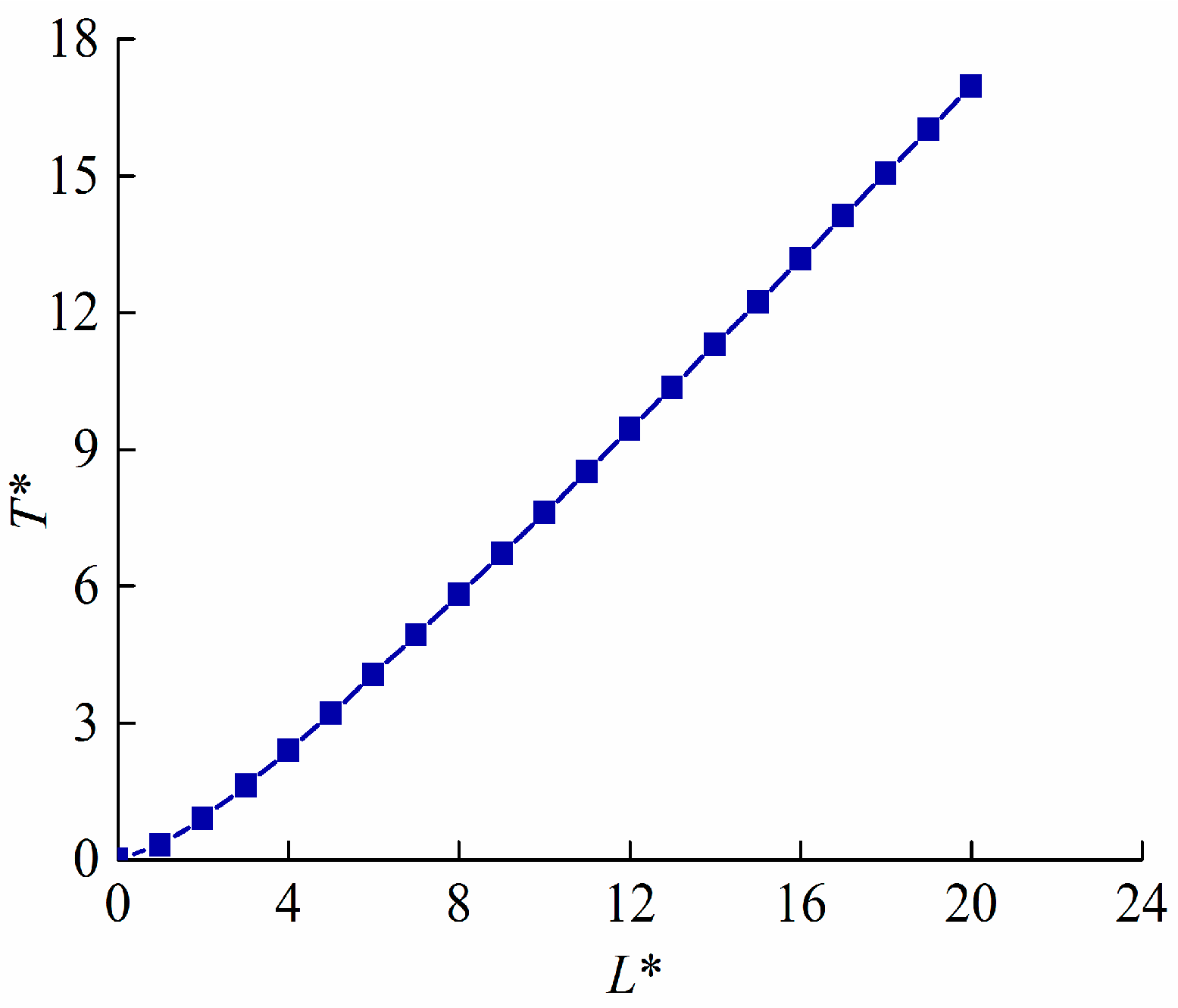
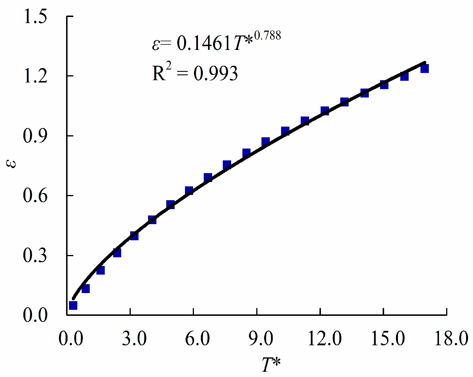
2.4. Proposed Model
3. Materials and Methods
3.1. Laboratory Experiment
3.2. Numerical Simulation
3.3. Criteria for Model Evaluation
4. Results and Discussion
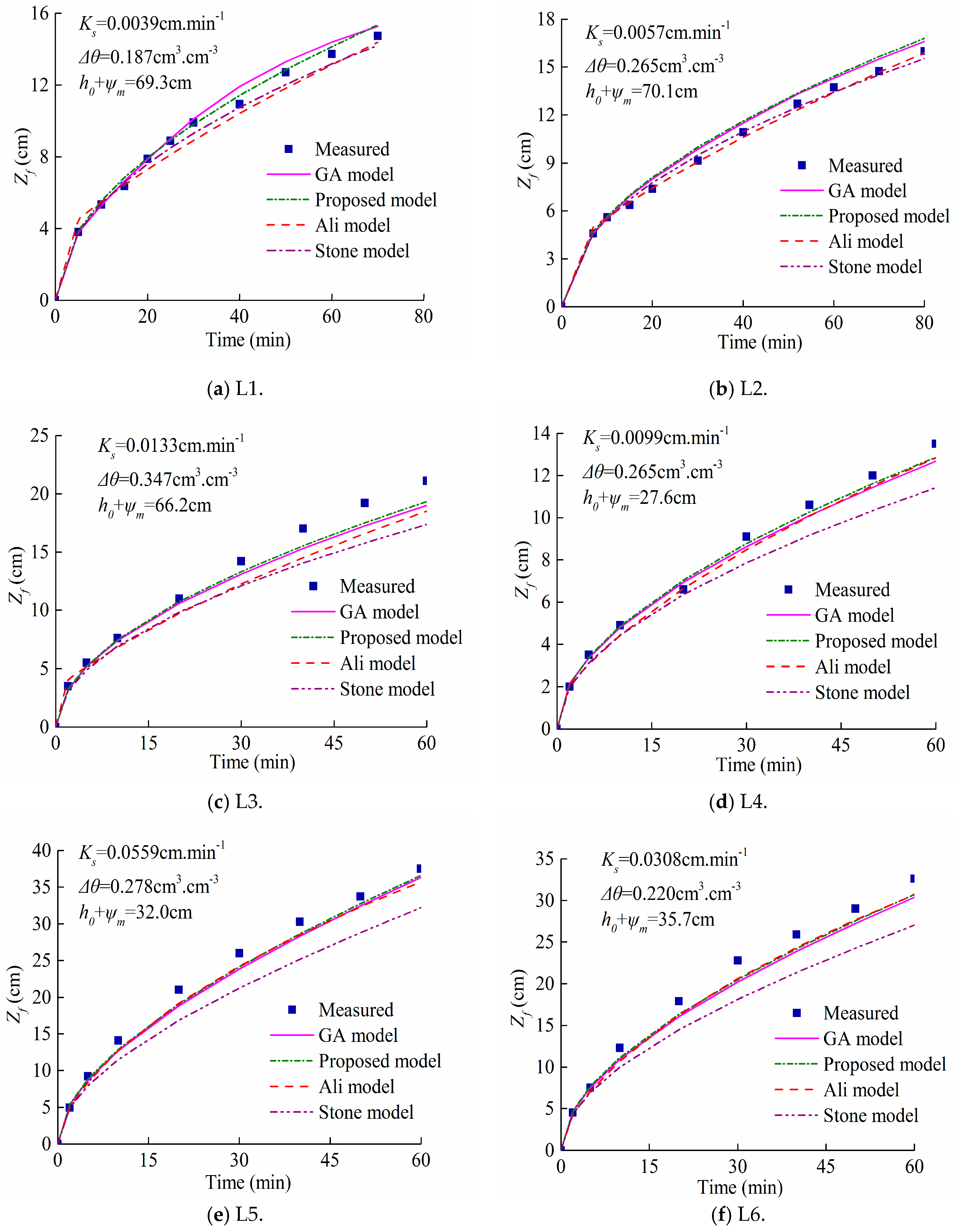
4.1. Comparison of the Four Models Using Measured Values of Zf
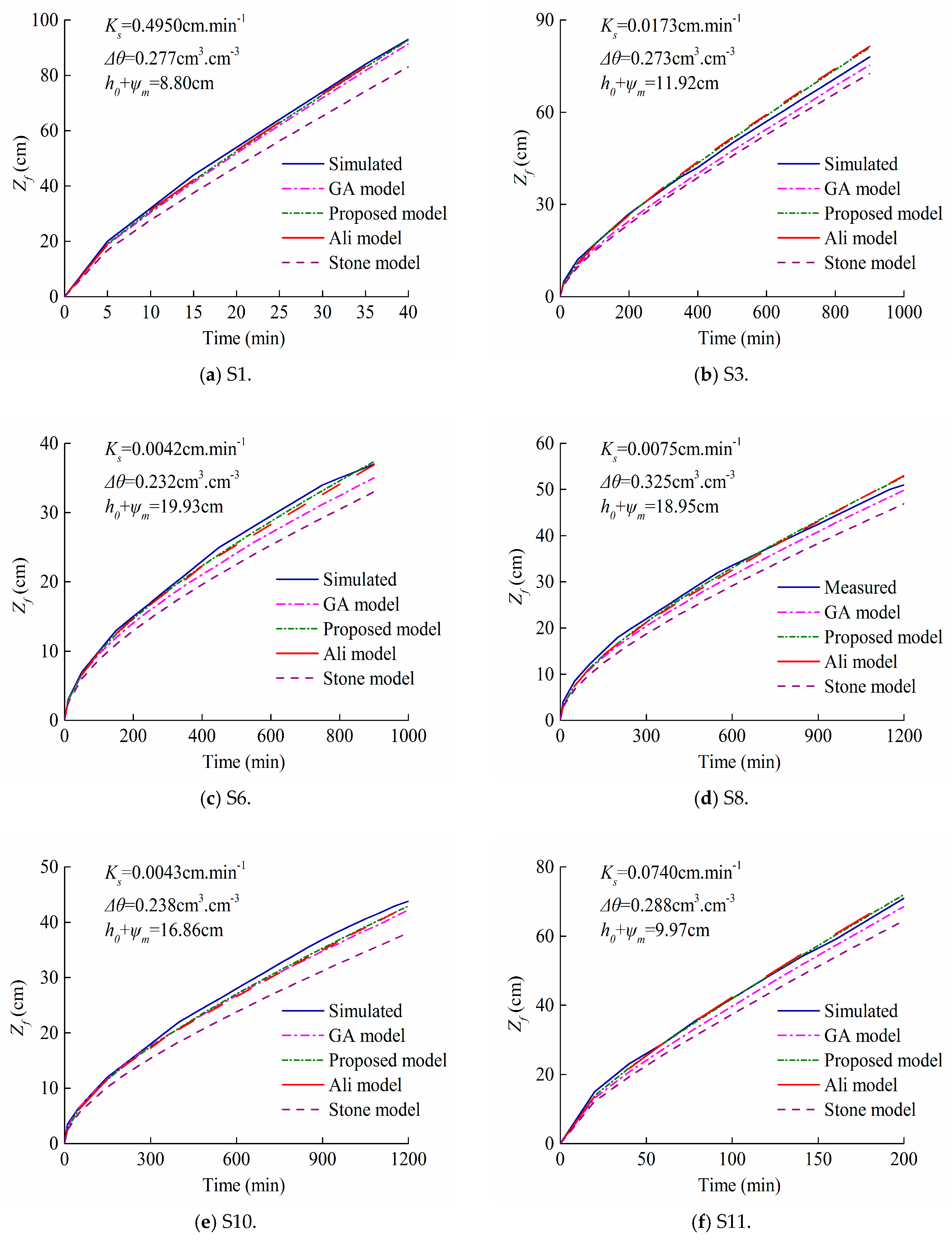
4.2. Comparison of the Four Models Using HYDRUS-1D-Simulated Values of Zf
4.3. Comparison and Discussion of the Four Models
5. Conclusions
Acknowledgments
Author Contributions
Conflicts of Interest
References
- Mishra, S.K.; Tyagi, J.V.; Singh, V.P. Comparison of infiltration models. Hydrol. Process. 2003, 17, 2629–2652. [Google Scholar] [CrossRef]
- Ali, S.; Islam, A.; Mishra, P.K.; Sikka, A.K. Green-Ampt approximations: A comprehensive analysis. J. Hydrol. 2016, 535, 340–355. [Google Scholar] [CrossRef]
- Hu, H.P.; Gao, L.; Tian, F.Q. Empirical equation for development of soil wetted body under surface drip irrigation condition. J. Tsinghua Univ. Sci. Technol. 2010, 50, 839–843. [Google Scholar]
- Nie, W.B.; Ma, X.Y.; Wang, S.L. Forecast model for wetting front migration distance under furrow irrigation infiltration. Trans. Chin. Soc. Agric. Eng. 2009, 25, 20–25. [Google Scholar]
- Xiong, Y.W.; Furman, A.; Wallach, R. Moment analysis description of wetting and redistribution plumes in wettable and water-Repellent soils. J. Hydrol. 2012, 422, 30–42. [Google Scholar] [CrossRef]
- Zhang, Y.Y.; Zhao, X.N.; Wu, P.T. Soil wetting patterns and water distribution as affected by irrigation for uncropped ridges and furrows. Pedosphere 2015, 25, 468–477. [Google Scholar] [CrossRef]
- Rao, M.D.; Raghuwanshi, N.S.; Singh, R. Development of a physically based 1D-Infiltration model for seal formed irrigated soils. Agric. Water Manag. 2006, 84, 164–174. [Google Scholar]
- Valiantzas, D.; Pollalis, E.D.; Soulis, K.X.; Londra, P.A. Rapid graphical detection of weakness problems in numerical simulation infiltration models using a linearizes form equation. J. Irrig. Drain. Eng. ASCE 2011, 137, 524–529. [Google Scholar] [CrossRef]
- Malek, K.; Peters, R.T. Wetting pattern models for drip irrigation: New empirical model. J. Irrig. Drain. Eng. ASCE 2011, 137, 530–536. [Google Scholar] [CrossRef]
- Rasheeda, S.; Sasikumar, K. Modelling vertical infiltration in an unsaturated porous media using neural network architecture. Aquat. Procedia 2015, 4, 1008–1015. [Google Scholar] [CrossRef]
- Green, W.H.; Ampt, G. Study on soil physics-1. The flow of air and water through soils. J. Agric. Sci. 1911, 4, 1–24. [Google Scholar]
- Philip, J. Plant water relations: Some physical aspects. Annu. Rev. Plant Physiol. 1966, 17, 245–268. [Google Scholar] [CrossRef]
- Stone, J.J.; Hawkins, R.H.; Shirley, E.D. Approximate form of Green-Ampt infiltration equation. J. Irrig. Drain. Eng. ASCE 1994, 120, 128–137. [Google Scholar] [CrossRef]
- Enciso-Medina, J.; Martin, D.; Eisenhauer, D. Infiltration model from furrow irrigation. J. Irrig. Drain. Eng. ASCE 1998, 124, 73–80. [Google Scholar] [CrossRef]
- Li, R.M.; Steven, M.A.; Simons, D.B. Solutions to Green-Ampt infiltration equation. J. Irrig. Drain. Eng. Div. ASCE 1976, 102, 239–248. [Google Scholar]
- Salvucci, G.D.; Entekhabi, D. Explicit expressions for Green-Ampt (delta function diffusivity) infiltration rate and cumulative storage. Water Resour. Res. 1994, 30, 2661–2663. [Google Scholar] [CrossRef]
- Barry, D.A.; Parlange, J.Y.; Sander, G.C.; Sivapalan, M. Comment on explicit expression for Green-Ampt (delta function diffusivity) infiltration rate and cumulative storage. Water Resour. Res. 1995, 31, 1445–1446. [Google Scholar] [CrossRef]
- Serrano, S.E. Explicit solution to Green and Ampt infiltration equation. J. Hydrol. Eng. 2001, 6, 336–340. [Google Scholar] [CrossRef]
- Chen, L.; Young, M.H. Green-Ampt infiltration model for sloping surfaces. Water Resour. Res. 2006, 42, 887–896. [Google Scholar] [CrossRef]
- Mailapalli, D.R.; Wallender, W.W.; Singh, R.; Raghuwanshi, N.S. Application of a nonstandard explicit integration to solve Green and Ampt infiltration equation. J. Hydrol. Eng. 2009, 14, 203–206. [Google Scholar] [CrossRef]
- Almedeij, J.; Esen, I.I. Modified Green-Ampt infiltration model for steady rainfall. J. Hydrol. Eng. 2014, 19, 04014011. [Google Scholar] [CrossRef]
- Zhu, J.T.; Ogden, F.L.; Lai, W.C.; Chen, X.F.; Talbot, C.A. An explicit approach to capture diffusive effects in finite water-Content method for solving vadose zone flow. J. Hydrol. 2016, 535, 270–281. [Google Scholar] [CrossRef]
- Youngs, E.G. An estimation of sorptivity for infiltration studies from moisture moments considerations. Soil Sci. 1968, 106, 157–163. [Google Scholar] [CrossRef]
- Philip, J.R. Theory of infiltration. Adv. Hydrosci. 1969, 5, 215–296. [Google Scholar]
- Talsma, T.; Parlange, J.Y. One-Dimensional vertical infiltration. Aust. J. Soil Res. 1972, 10, 143–150. [Google Scholar] [CrossRef]
- Fuentes, C.; Haverkamp, R.; Parlange, J.Y. Parameter constraints on closedform soil-Water relationships. J. Hydrol. 1992, 134, 117–142. [Google Scholar] [CrossRef]
- Ali, S.; Ghosh, N.C.; Singh, R.; Sethy, B.K. Generalized explicit models for estimation of wetting front length and potential recharge. Water Resour. Manag. 2013, 27, 2429–2445. [Google Scholar] [CrossRef]
- Bouwer, H. Groundwater Hydrology, 1st ed.; Wiley: New York, NY, USA, 1978. [Google Scholar]
- Bautista, E.; Warrick, A.W.; Strelkoff, T.S. New results for an approximate method for calculating two-Dimensional furrow infiltration. J. Irrig. Drain. Eng. ASCE 2014, 140, 04014032. [Google Scholar] [CrossRef]
- Philip, J.R. The theory of infiltration: 4. Sorptivity and algebraic infiltration equations. Soil Sci. 1957, 84, 257–264. [Google Scholar] [CrossRef]
- Valiantzas, J.D. New linearized two-parameter infiltration equation for direct determination of conductivity and sorptivity. J. Hydrol. 2010, 384, 1–13. [Google Scholar] [CrossRef]
- Esfandiari, M.; Maheshwari, B.L. Field values of shape factor for estimating surface storage in furrows on a clay soil. Irrig. Sci. 1997, 17, 157–161. [Google Scholar] [CrossRef]
- Nie, W.B.; Fei, L.J.; Ma, X.Y. Impact of infiltration parameters and Manning roughness on the advance trajectory and irrigation performance for closed-end furrows. Span. J. Agric. Res. 2014, 12, 1180–1191. [Google Scholar] [CrossRef]
- Fok, Y.S.; Chiang, H.S. 2-D infiltration equations for furrow irrigation. J. Irrig. Drain. Div. ASCE 1984, 110, 209–217. [Google Scholar] [CrossRef]
- Nie, W.B.; Ma, X.Y.; Wang, S.L. Numerical simulation of one-dimensional soil infiltration characteristic. J. Irrig. Drain. Eng. 2009, 28, 53–57. [Google Scholar]
- Warrick, A.W. Soil Water Dynamics; Oxford University Press: New York, NY, USA, 2003. [Google Scholar]
- HYDRUS-1D, version 4.0; PC-Progress: Prague, Czech Republic, 2007.
- Van Genuchten, M.Th. A closed-form equation for predicting the hydraulic conductivity of unsaturated soils. Soil Sci. Soc. Am. J. 1980, 44, 892–898. [Google Scholar] [CrossRef]
- Carsel, R.F.; Parrish, R.S. Developing joint probability distributions of soil water retention characteristics. Water Resour. Res. 1988, 24, 755–769. [Google Scholar] [CrossRef]
- Moriasi, D.; Arnold, J.; Liew, M.W.V.; Veith, T.L. Model evaluation guidelines for systematic quantification of accuracy in watershed simulations. Trans. Am. Soc. Agric. Biol. Eng. 2007, 50, 885–900. [Google Scholar] [CrossRef]
- Zhang, Y.Y.; Wu, P.T.; Zhao, X.N.; Wang, Z.K. Simulation of soil water dynamics for uncropped ridges and furrows under irrigation conditions. Can. J. Soil Sci. 2013, 93, 85–98. [Google Scholar] [CrossRef]
- Jacovides, C.P.; Kontoyiannis, H. Statistical procedures for the evaluation of evapotranspiration computing models. Agric. Water Manag. 1995, 27, 365–371. [Google Scholar] [CrossRef]
- Nayak, P.C.; Sudheer, K.P.; Rangan, D.M.; Ramasastri, K.S. A neuro-fuzzy computing technique for modelling hydrological time series. J. Hydrol. 2004, 291, 52–66. [Google Scholar] [CrossRef]
- Ma, J.J.; Sun, X.H.; Guo, X.H. Varying head infiltration model based on Green-Ampt model and solution to its key parameters. J. Hydrol. Eng. 2010, 41, 61–67. [Google Scholar]
- Mao, L.L.; Lia, Y.Z.; Hao, W.P.; Zhou, X.N.; Xu, C.Y.; Lei, T.W. A new method to estimate soil water infiltration based on a modified Green-Ampt model. Soil Tillage Res. 2016, 161, 31–37. [Google Scholar] [CrossRef]

| No. | Soil Texture | γd (g cm−3) | θ0 (cm3 cm−3) | θs (cm3 cm−3) | Δθ (cm3 cm−3) | h0 (cm) | ψm (cm) | h0 + ψm (cm) | Ks (cm min−1) | T (min) |
|---|---|---|---|---|---|---|---|---|---|---|
| L1 | Clay | — | — | — | 0.187 | — | — | 69.3 | 0.0039 | 70 |
| L2 | — | — | — | 0.265 | — | — | 70.1 | 0.0057 | 80 | |
| L3 | Clay loam | 1.3 | 0.156 | 0.503 | 0.347 | 5.5 | 60.7 | 66.2 | 0.0133 | 60 |
| L4 | 1.4 | 0.168 | 0.433 | 0.265 | 10.5 | 17.1 | 27.6 | 0.0099 | 60 | |
| L5 | Sandy loam | 1.4 | 0.098 | 0.376 | 0.278 | 10.5 | 21.5 | 32.0 | 0.0559 | 60 |
| L6 | 1.5 | 0.135 | 0.355 | 0.220 | 5.5 | 30.2 | 35.7 | 0.0308 | 60 |
| Soil Texture | θr (cm3 cm−3) | θS (cm3 cm−3) | a (cm−1) | l | n | Ks (cm min−1) |
|---|---|---|---|---|---|---|
| Sand | 0.045 | 0.430 | 0.145 | 0.5 | 2.680 | 0.4950 |
| Loam | 0.078 | 0.430 | 0.036 | 0.5 | 1.560 | 0.0173 |
| Silt | 0.034 | 0.460 | 0.016 | 0.5 | 1.370 | 0.0042 |
| Silt loam | 0.067 | 0.450 | 0.020 | 0.5 | 1.410 | 0.0075 |
| Clay loam | 0.095 | 0.410 | 0.019 | 0.5 | 1.310 | 0.0043 |
| Sandy loam | 0.065 | 0.410 | 0.075 | 0.5 | 1.890 | 0.0740 |
| No. | Soil Texture | θ0 (cm3 cm−3) | Δθ (cm3 cm−3) | h0 (cm) | ψm (cm) | t (min) |
|---|---|---|---|---|---|---|
| S1 | Sand | 0.153 | 0.277 | 5 | 3.80 | 40 |
| S2 | 10 | |||||
| S3 | Loam | 0.157 | 0.273 | 5 | 6.92 | 900 |
| S4 | 10 | |||||
| S5 | Silt | 0.228 | 0.232 | 5 | 9.93 | 900 |
| S6 | 10 | |||||
| S7 | Silt loam | 0.125 | 0.325 | 5 | 8.95 | 1200 |
| S8 | 10 | |||||
| S9 | Clay loam | 0.172 | 0.238 | 5 | 6.86 | 1200 |
| S10 | 10 | |||||
| S11 | Sandy loam | 0.122 | 0.288 | 5 | 4.97 | 200 |
| S12 | 10 |
| No. | GA Model | Proposed Model | Ali Model | Stone Model | ||||||||
|---|---|---|---|---|---|---|---|---|---|---|---|---|
| RMSE (cm) | MAPRE (%) | PB (%) | RMSE (cm) | MAPRE (%) | PB (%) | RMSE (cm) | MAPRE (%) | PB (%) | RMSE (cm) | MAPRE (%) | PB (%) | |
| L1 | 0.47 | 3.17 | 3.55 | 0.34 | 2.87 | 2.60 | 0.64 | 6.73 | −4.09 | 0.59 | 4.89 | −5.26 |
| L2 | 0.57 | 4.64 | 4.98 | 0.68 | 5.56 | 6.12 | 0.24 | 2.05 | −0.59 | 0.37 | 2.75 | −2.20 |
| L3 | 1.26 | 6.46 | −8.12 | 1.07 | 5.25 | −6.74 | 1.81 | 10.96 | −11.54 | 2.27 | 12.17 | −15.19 |
| L4 | 0.45 | 4.44 | −3.41 | 0.35 | 3.40 | −2.03 | 0.47 | 5.44 | −4.90 | 1.18 | 9.04 | −12.08 |
| L5 | 1.53 | 6.17 | −5.79 | 1.30 | 5.44 | −4.74 | 1.45 | 5.41 | −6.01 | 3.97 | 12.84 | −15.85 |
| L6 | 1.73 | 6.32 | −7.61 | 1.49 | 5.89 | −6.35 | 1.50 | 6.52 | −7.11 | 3.76 | 13.33 | −17.01 |
| Mean value | 1.00 | 5.20 | −2.73 | 0.87 | 4.73 | −1.86 | 1.02 | 6.18 | −5.71 | 2.02 | 9.17 | −11.27 |
| No. | GA Model | Proposed Model | Ali Model | Stone Model | ||||||||
|---|---|---|---|---|---|---|---|---|---|---|---|---|
| RMSE (cm) | MAPRE (%) | PB (%) | RMSE (cm) | MAPRE (%) | PB (%) | RMSE (cm) | MAPRE (%) | PB (%) | RMSE (cm) | MAPRE (%) | PB (%) | |
| S1 | 1.98 | 4.16 | −3.33 | 1.21 | 1.75 | −1.91 | 0.99 | 2.07 | −1.49 | 7.48 | 11.13 | −12.26 |
| S2 | 1.67 | 3.73 | −1.97 | 1.58 | 2.52 | −1.84 | 1.42 | 2.37 | −1.30 | 8.12 | 12.84 | −12.34 |
| S3 | 2.26 | 6.49 | −4.91 | 1.74 | 3.33 | 2.66 | 2.07 | 4.10 | 3.18 | 3.92 | 10.09 | −8.39 |
| S4 | 2.13 | 5.84 | −4.16 | 0.97 | 2.86 | 0.46 | 1.38 | 3.64 | 0.94 | 5.56 | 11.41 | −10.59 |
| S5 | 3.09 | 17.36 | −14.03 | 1.21 | 6.76 | −4.28 | 1.35 | 7.64 | −5.28 | 3.41 | 17.18 | −15.55 |
| S6 | 1.93 | 8.56 | −7.43 | 0.58 | 2.51 | −1.99 | 0.86 | 3.67 | −3.16 | 3.44 | 13.58 | −13.63 |
| S7 | 2.06 | 10.21 | −7.08 | 1.62 | 5.56 | 2.14 | 1.82 | 6.37 | 2.10 | 2.71 | 12.06 | −9.43 |
| S8 | 1.68 | 7.04 | −5.17 | 0.89 | 3.84 | −0.14 | 1.02 | 4.56 | −0.77 | 3.80 | 13.46 | −11.67 |
| S9 | 3.24 | 13.95 | −11.87 | 1.56 | 6.92 | −5.90 | 1.59 | 7.56 | −6.12 | 4.48 | 17.61 | −16.69 |
| S10 | 1.44 | 4.90 | −4.56 | 1.07 | 4.39 | −3.61 | 1.32 | 5.50 | −4.45 | 4.40 | 15.51 | −14.89 |
| S11 | 2.15 | 6.31 | −4.82 | 0.83 | 2.04 | 0.23 | 1.05 | 2.50 | 0.74 | 4.77 | 11.60 | −10.50 |
| S12 | 1.92 | 4.78 | −3.84 | 0.70 | 1.77 | −0.91 | 0.87 | 2.08 | −0.37 | 6.03 | 12.57 | −11.78 |
| Mean value | 2.13 | 7.78 | −6.10 | 1.16 | 3.69 | −1.26 | 1.31 | 4.34 | −1.33 | 4.84 | 13.25 | −12.31 |
© 2017 by the authors. Licensee MDPI, Basel, Switzerland. This article is an open access article distributed under the terms and conditions of the Creative Commons Attribution (CC BY) license (http://creativecommons.org/licenses/by/4.0/).
Share and Cite
Nie, W.-B.; Li, Y.-B.; Fei, L.-J.; Ma, X.-Y. Approximate Explicit Solution to the Green-Ampt Infiltration Model for Estimating Wetting Front Depth. Water 2017, 9, 609. https://doi.org/10.3390/w9080609
Nie W-B, Li Y-B, Fei L-J, Ma X-Y. Approximate Explicit Solution to the Green-Ampt Infiltration Model for Estimating Wetting Front Depth. Water. 2017; 9(8):609. https://doi.org/10.3390/w9080609
Chicago/Turabian StyleNie, Wei-Bo, Yi-Bo Li, Liang-Jun Fei, and Xiao-Yi Ma. 2017. "Approximate Explicit Solution to the Green-Ampt Infiltration Model for Estimating Wetting Front Depth" Water 9, no. 8: 609. https://doi.org/10.3390/w9080609
APA StyleNie, W.-B., Li, Y.-B., Fei, L.-J., & Ma, X.-Y. (2017). Approximate Explicit Solution to the Green-Ampt Infiltration Model for Estimating Wetting Front Depth. Water, 9(8), 609. https://doi.org/10.3390/w9080609