Hourly Water Level Forecasting at Tributary Affected by Main River Condition


1
Han River Flood Control Office, Ministry of Land, Infrastructure and Transport (MOLIT), 328 Dongjak-daero, Seocho-Gu, Seoul 06501, Korea
2
School of Civil & Environmental Engineering, College of Engineering, Yonsei University, 50 Yonsei-ro Seodaemun-Gu, Seoul 03722, Korea
3
Hydro Science and Engineering Research Institute, Korea Institute of Civil Engineering and Building Technology (KICT), 283 Goyang-daero, Ilsanseo-Gu, Goyang-Si 10223, Gyeonggi-Do, Korea
*
Author to whom correspondence should be addressed.
Water 2017, 9(9), 644; https://doi.org/10.3390/w9090644
Submission received: 18 August 2017
/
Revised: 18 August 2017
/
Accepted: 21 August 2017
/
Published: 28 August 2017
Abstract
:This study develops hourly water level forecasting models with lead-times of 1 to 3 h using an artificial neural network (ANN) for Anyangcheon stream, one of the major tributaries of the Han River, South Korea. To consider the backwater effect from this river, an enhanced tributary water level forecasting model is proposed by adding multiple water level data on the main river as input variables into the conventional ANN structure which often uses rainfall and upstream water level data. Four types of ANN models per each lead-time are built with increasing complexity of the input vector, and their performances are compared. The results indicate that the inclusion of multiple water level data on the main river to the network provides water level forecasts with greater accuracy at the Ogeumgyo gauging station of interest. The final best ANN models for water level forecasts with lead-times of 1 to 2 h show good performance with root mean square errors (RMSE) below 0.06 m and 0.12 m, respectively. However, the final best ANN model for forecasting 3 h ahead was unsatisfactory, showing underestimation at many rising parts of the hydrograph.
1. Introduction
Flood forecasting in rivers is an essential non-structural countermeasure against flood disasters [1]. For this purpose, flood forecasting is usually performed using process-based models, which require basic data collection and periodic data updating. Careful model calibration is essential for simulating actual flood events. However, as the number of parameters increases, more time is needed to ensure sufficient accuracy in the model predictions [2,3,4,5]. To predict flood water levels in small urban watersheds, which vary abruptly according to rainfall, careful decisions must be declared within a few hours. Thus, more efficient methodology should be chosen to predict water levels in urban stream and tributaries in a few hours. Accordingly, process-based methodologies such as complex physical models have limitations regarding flood warning because the running time for such modeling is generally too long [6].
One alternative for solving this limitation is to use an artificial neural network (ANN) model for predicting water levels. ANN belongs to a class of data-driven models rather than process-based conceptual or physical models [7,8] and has been widely used for flood prediction since the early 1990s [9,10,11], alone or coupled with a process-based model to reduce error [12,13,14]. Moreover, researchers have applied various techniques of neural network models to obtain better prediction accuracy [15]. The many types of neural network model applications include typical backpropagation ANN (BP-ANN) [16], feedforward neural network (FFNN) using multilayer perceptron (MLP) and radial basis function network (RBF) [17], and recurrent neural network (RNN) [18] as dynamic models. Theoretical improvement trials enable researchers to apply ANN models for various applications.
In recent years, the utility of ANN models in simulating complex hydrological conditions has provided various opportunities for flood prediction by focusing on the water level in inundation areas [19], peak flow prediction in urban areas [20], water levels in areas having insufficient data [21], and conditions of irregular rainfall and runoff [22].
Flood prediction in large rivers has a high degree of accuracy, whereas in small tributary rivers is limited owing to the short travel time through the basin [23]. In such small rivers, hourly data prediction is crucial for ensuring good lead-time to the flood response. ANN has shown good accuracy for watersheds with short concentration times [24]. For researching hourly river stage forecasts, a wavelet bootstrap ANN model was applied with reasonable results [25]. Lizhen. [26] analyzed various model settings in a series of artificial models including ANN for hourly water level prediction against flash flooding. Regarding tributary rivers, MinChiang River in China is subject to flooding because the main river has several tributaries [27]. Tributaries are influenced by the backwater effect from a main river, which makes prediction more complex. The backwater effect is considered in physical models [28]; therefore, these models are essential for predicting the flood level in tributary rivers that include this effect. In this study, an enhanced water level prediction model is proposed by adding the backwater effect from the main stream into the conventional training process of ANN model in which rainfall and upstream water level data are used. The present study focuses on short-term water level forecasting with lead-times of 1 to 3 h using ANN models. This study demonstrates that forecasts can be improved if water level data in the main river is included in the ANN model construction. To this end, ANN models for hourly water level forecasting are developed and their performance is investigated for Anyangcheon stream, a major tributary of the Han River, South Korea.
2. Materials and Methods
2.1. Study Area and Used Data
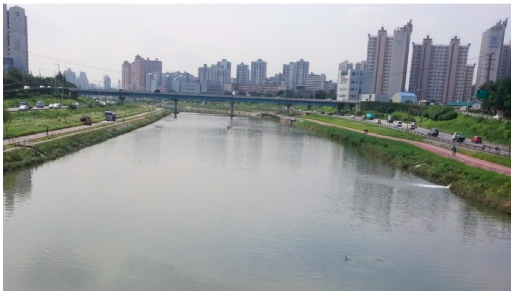
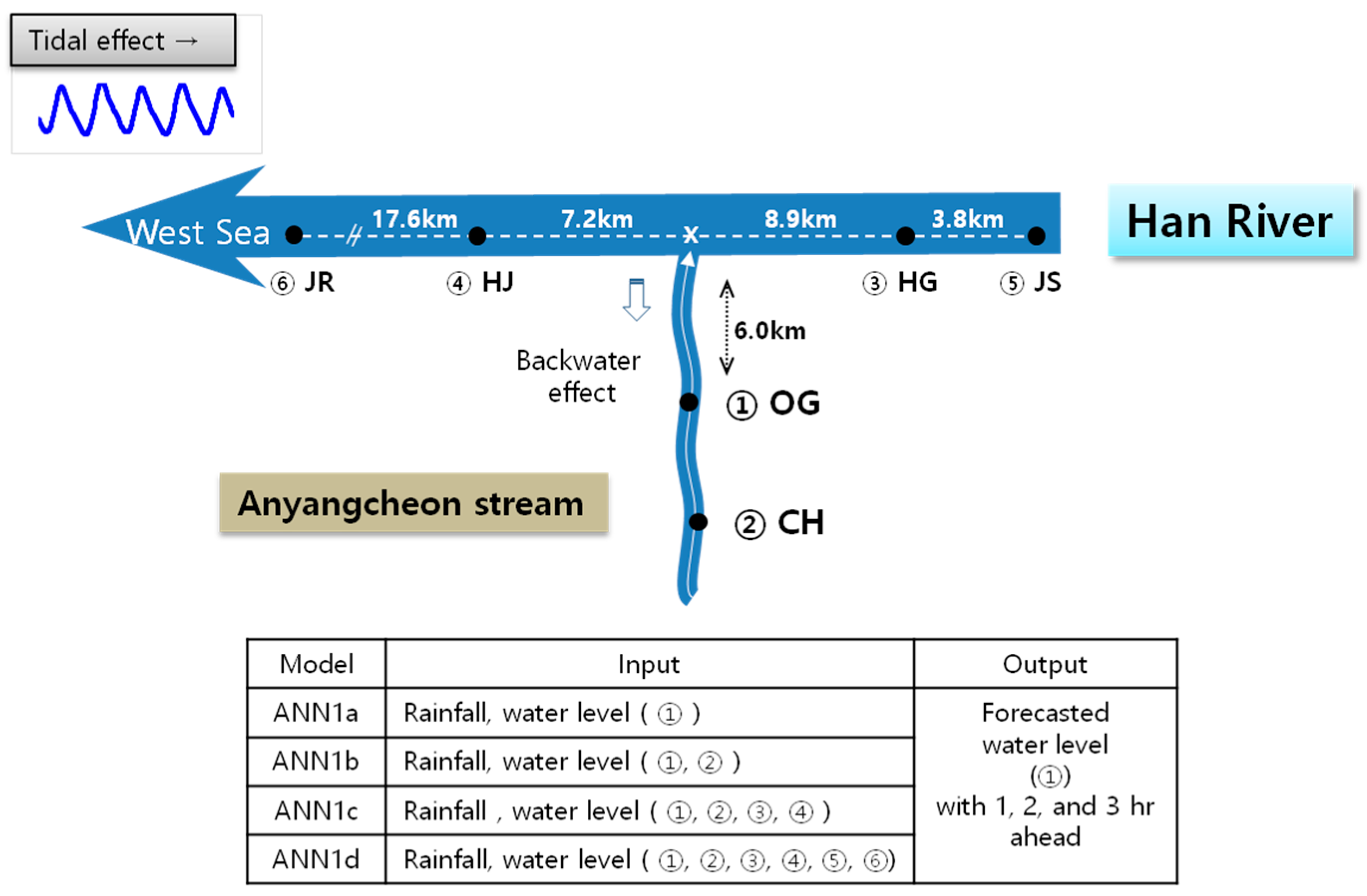
Anyangcheon stream is a tributary of the Han River (Figure 1). Located at the southwest part of the Seoul metropolitan area, the study area is the Anyangcheon stream watershed (Figure 2), having an area of 286 km2 and a main channel length of 32.5 km. Because many residential (urbanized) districts are situated in the upstream (downstream) area, reliable flood warning is crucial to mitigate damage in this area. Ogeumgyo Bridge, the flood prediction site located 6 km upstream of the junction of the Han River, is significantly affected by the backwater effect from the river. Flood flow in the Han River is largely influenced by the release from Paldang reservoir and the tidal effect from sea water at the end of the river. Moreover, a series of tributaries such as Wangsukcheon, Tancheon, Jungnangcheon, and Anyangcheon streams flow to the Han River.
In this study, to predict flood water levels at the Ogeumgyo Bridge, hourly rainfall and water level data were used. Water level data from four gauging stations at the Han River were used to consider the backwater effect from the river, which is affected by release from Paldang reservoir and tidal conditions. To compute average rainfall, a Thiessen polygon was constructed including nine rainfall gauging stations. Data used for this study include hourly water level series from six gauging stations of Ogeumgyo (OG), Chunghungyo (CH), Jeonryu (JR), Haengjudaegyo (HJ), Hangangdaegyo (HG), and Jamsugyo (JS) and basin-averaged hourly rainfall series obtained from the Water Management Information System (WAMIS) provided by the Ministry of Land, Infrastructure and Transport (MOLIT), South Korea. The locations of the gauging stations are shown in Figure 2 and Figure 3. This study focused on water level forecasts during the rainy season. Only data recorded during the monsoon period from 21 June to 20 September for 2007–2016 were used in this study because this period is considered as the main rainy season in South Korea. These data collected were divided into two subsets. Data from the first six years were used for training, whereas those from the remaining four years were used for testing the model.
2.2. Artificial Neural Network Model
The human brain is made up of huge networks of complex neurons connected by a substance called synapse and is able to define its own rules based on experience. Inspired by the structure of the human brain, McCulloch and Pitts first proposed an ANN [29], and various ANN models have since been developed. An ANN model is a data-driven mathematical model having the ability to solve problems by learning neurons without inputting direct knowledge or physical processes. The ANN model is capable of identifying complex nonlinear relationships between inputs and outputs without needing to understand the nature of the phenomenon [30].
The most widely used neural network is the multilayer perceptron [30] (Figure 4), in which neurons are organized in input, hidden, and output layers interconnected by their own connection strengths. The network is optimized through training. Computation of the ANN outputs the weighted sum of external stimuli entering the input layer through the activation function. ANN is considered to be a fairly simple and cost-effective tool for obtaining solutions through the procedures of defining distributions, training, and validation.
The three-layered feed forward neural network which has been widely used in hydrologic forecasting models can be represented by a linear combination of the transformed input variables as:
where is the forecasted th output value, is the activation function for the output neuron, is the number of output neurons, is the weight connecting the th neuron in the hidden layer and th neuron in the output layer, is the activation function for the hidden neuron, is the number of hidden neurons, is the weight connecting the th neuron in the input layer and th neuron in the hidden layer, is the th input variable, is the bias for the th hidden neuron, and is the bias for the th th output neuron [31]. Neural networks can learn their weights and biases through a training process. In the present study, ANN weights and biases were updated by a back-propagation algorithm which was developed originally by Rumelhart et al. (1986) [32]. The algorithm is based on the gradient descent method with the objective of minimizing the sum of errors of the network in Equation (2).
where is the error for all input patterns, is the error based on the squared difference between target outputs and forecasted outputs for pattern p [33].
2.3. ANN Model Development
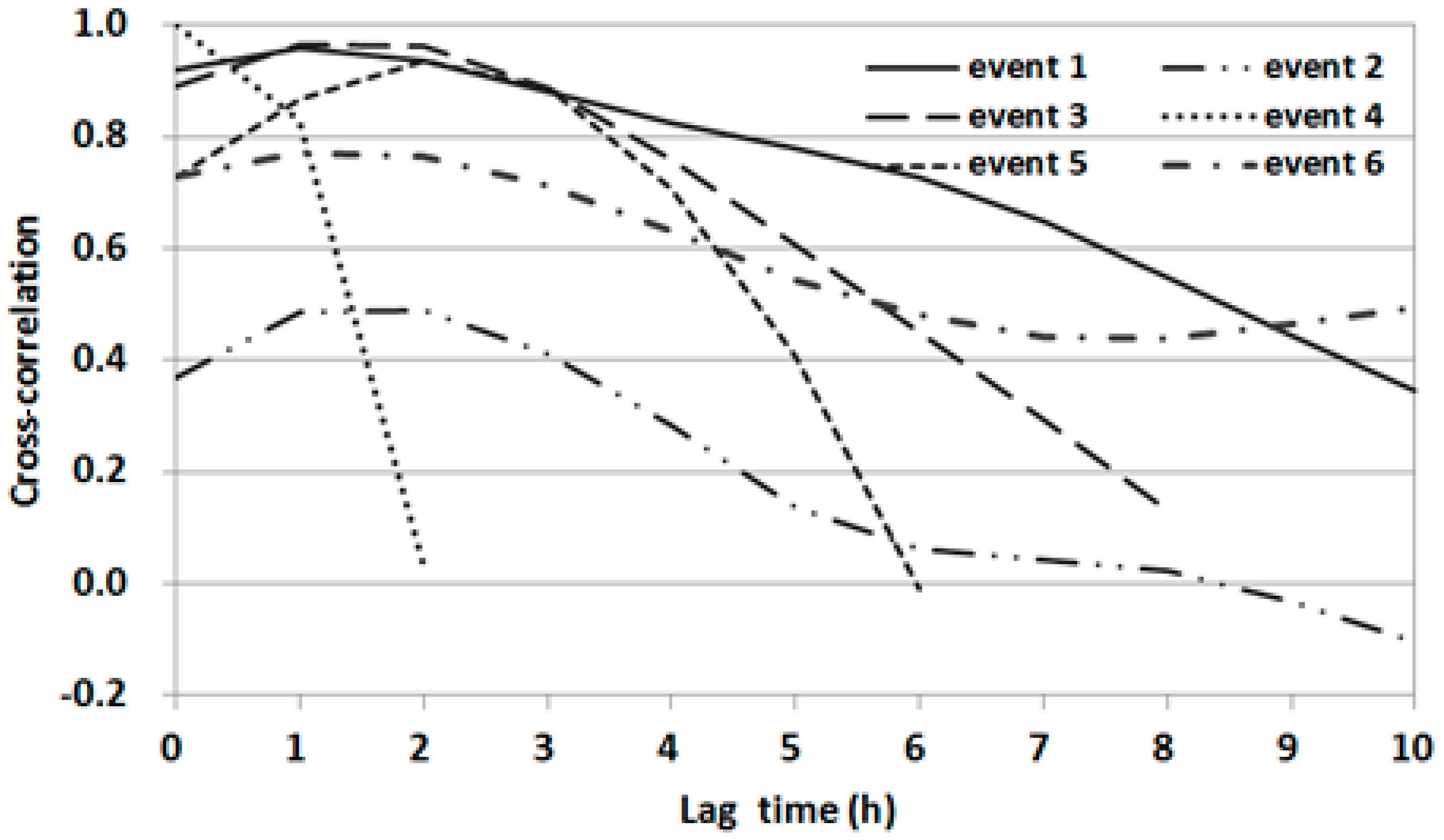
In this study, three types of ANN models were built to forecast water levels with 1, 2, and 3 h lead-times, respectively. The two most important steps in the ANN model development are the selection of significant input variables and the optimization of network architecture. Usually, significant input variables of networks can be determined through statistical analysis of data series such as the cross-correlation function (CCF), auto-correlation function (ACF), and partial auto-correlation function (PACF), as suggested by Sudheer and Jain [34]. In this study, correlation analyses were performed for total period data, and Figure 5, Figure 6, Figure 7 and Figure 8 illustrated the results for six events given in Table 1.
The CCFs between the water level series at output station OG and the areal rainfall series for six flood events are shown in Figure 5. The magnitudes of CCF values varied considerably with the lag time for each event. Events 1 and 4 showed a high correlation with 2 h of lag time in the water level data on averaged rainfall data at any time. However, event 5 showed significant correlation with 3 to 5 h of lag time. A specific dominant cross-correlation process could not be determined. Furthermore, very low CCFs were found for events 2 and 6 even though the events showed high peaks. This might be attributed to an effect of the boundary conditions of the water level at the confluence of the tributary of interest and the main river.
The CCFs between the water level at OG and the upstream water level at CH were estimated for each event, as shown in Figure 6. The CCF for event 1 showed a significant correlation with a lag time of up to 7 h, whereas those for events 3, 5, and 6 showed significant correlation with lag times of up to 4 h. For event 4, which had short flood duration, the CCF rapidly declined after a lag time of 2 h. The low CCF for event 2 indicated that the water level could be affected by other factors such as downstream hydrologic conditions.
The CCF between the water level at OG and that at HJ located on the main river is shown in Figure 7. A highly significant correlation was found for events 1, 2, and 6. The CCFs decreased gradually with an increase in lag time, which indicates that the output water level data at OG are strongly correlated with the water level data on the main river. The same processes were applied to estimate the CCFs between the output and input variables of water levels at JR, HG, and JS, which also showed various correlations for each event.
The ACFs from 0 to 10 h lag times were estimated for the water level data at OG. A significant correlation up to about 8 h of lag time was found for events 1 and 6 (Figure 8). However, the ACF for event 4 decreased sharply after 1 h of lag time. As shown in Figure 8, the ACFs differed significantly among events and decreased gradually or rapidly with an increase in lag time.
On the basis of the statistical analysis of correlation presented above, the input and output data nonlinearly correlated with each other. This nonlinearity means that the backwater effect is inherent in the output data. In the case that backwater effect is apparent in target water level data, the ANN model will be useful to deal with nonlinear features. Weak cross-correlations for some events indicated that it might be difficult to determine the specific dominant lag time of input variables in advance in the case of our study area where backwater effect from the main river exists. Therefore, a trial and error procedure was used in this study to identify the optimal input vector using various lag times of input variables.
The optimal structure was determined by considering input variables from the current time (t) to previous hours (from t-1 to t-10). Statistical errors of the training set were calculated for the different number of nodes in the hidden layer. Liang and Sun [35] proposed that number of hidden neurons should be half size of the input nodes plus output nodes for better forecasting accuracy. According to this guide, the numbers of hidden nodes within 39 were tested considering the size of input nodes for the most complex ANN structure treated in the present study. The number of hidden nodes was progressively increased from 1 to 39, and then the ANN model performance was evaluated by the measure of root mean square error (RMSE). The results showed the minimum RMSE when the numbers of hidden nodes around 20 were used. Therefore, the optimal number of hidden nodes was determined to be between 1 and 20 in this study.
For each set of hidden nodes and input variables, the network was trained to minimize the root mean square error (RMSE) at one output layer by using a back-propagation algorithm. The learning rate was set to 0.01, and the hyperbolic tangent sigmoid function was used as the activation function for the hidden layer. The early stopping method has been widely used to avoid the over-fitting problem, in which, after dividing the data in three data sets, training, cross-validation, and testing, the output error of training and validation in each epoch is monitored and training is stopped when the cross-validation error is minimum [25]. However, the technique was not applied in the present study due to a large number of training cases for more than two thousands networks. A maximum epoch of 5000 was adopted for training, which was determined from the preliminary performance tests for the complex ANN structures.
ANN models were first trained by using the training data set, 60% of the total data, to obtain an optimized set of connection weights. These models were then tested by using the remaining data, 40% of the total data. These models were then compared by using three statistical measures: goodness of fit of RMSE, determination coefficient (R2), and Nash–Sutcliffe efficiency (NSE) given by
where is the observed water level, is the mean value, is the forecasted water level from the model, and N is the number of data points.
3. Results and Discussion
3.1. ANN Models for Hourly Water Level Forecasting with Lead-Times of 1 to 3 h
The water level at OG station is not only a function of rainfall but also an indicator of upstream and downstream hydrologic conditions. In this study, ANN models for forecasting hourly water levels with lead-times of 1 to 3 h were developed by combining rainfall, upstream water levels, and downstream water levels as input variables to the network.
The proposed ANN models and the associated input and output variables are given in Table 2. In the present work, ANN models were classified into four groups of (a)–(d) according to the input variables. In each group, three ANN models (i = 1, 2, 3) with lead-times of 1 to 3 h were developed. In Table 2, t is the current time, τ is the previous time, T is the lead-time, R is the catchment averaged rainfall, hOG is the water level at OG, hCH is the water level at CH, hHG is the water level at HG, hHJ is the water level at HJ, hJS is the water level at JS, and the hJR is the water level at JR.
As an example of an ANN model with a 1 h lead-time (i = 1) in Table 2, ANN1a uses data of water levels at the output target station (OG) and the watershed average rainfall. This model was first run without information on the upstream or downstream water levels. Then, ANN1b, ANN1c, and ANN1d were run by increasing the complexity of input step-by-step. In the ANN1b model, upstream water level data of CH () were added to the ANN1a model. In the ANN1c model, downstream water level data were added from two more gauging stations, HJ and HG, located about 7–9 km from the confluence of the tributary and the main river; this location is far from the outlet of Anyangcheon stream, about 6 km from the forecasted point. In the ANN1d model, downstream water level data at two more gauging stations, JR and JS, located farther from the confluence, were added to the ANN1c model.
In all models, the number of nodes in a hidden layer along with the number of previous hours was optimized manually for each model architecture after many trials. In the trial networks, the number of hidden nodes varied from 1 to 20, and the number of previous intervals also varied up to 10 h. The configuration that gave the minimum RMSE was primarily selected for 12 models including 4 models for each lead-time. For illustration, RMSEs of ANN1a and ANN3c models according to the number of hidden nodes and the previous time period for the training data set are shown in Figure 9a,b, respectively. As shown the figures, adopting the previous time spans of 3–5 h and 7 hidden nodes and 8 h with 17 hidden nodes produced the lowest RMSE values, respectively.
Finally, the number of neurons in a hidden layer and the number of previous time spans were determined after selecting an optimal configuration that produced the highest NSE and R2 among the primary selections that produced the lowest RMSE (Table 3).
3.2. Performance of ANN Models for 1 h Lead-Time Forecasting
The performances of four types of ANN models for 1 h lead-time forecasting are shown in Table 4. The statistical measurements for both training and testing sets showed that highly accurate water level forecasts could be obtained from each model. The RMSE was found to be very small. Both NSE and R2 were closer to unity for all ANN models using training and testing data sets. Of these four network models, ANN1d produced the best forecasting performance for both training and testing sets with the lowest RMSE values, 0.0585m and 0.0502m; the highest NSE, 0.9935 and 0.9864; and the highest R2, 0.9936 and 0.9868, respectively. The inclusion of upstream water level data resulted in only minor improvement (ANN1b). Inclusion of water level data of the main river after the confluence point (ANN1c and ANN1d) produced significantly improved forecasts.
For a flood warning system, the accuracy of the model forecasts is more important for high water levels than for medium-low water levels. To assess the performance of ANN models in forecasting high water levels, statistical measures were calculated for the 5% highest water level values, as given Table 5. These ANN models were found to be suitable for flood forecasting, and their performances could be improved by increasing the complexity of the input data. ANN1c and ANN1d models, including information of water level at the main river, showed lower RMSEs, below 0.09 m.
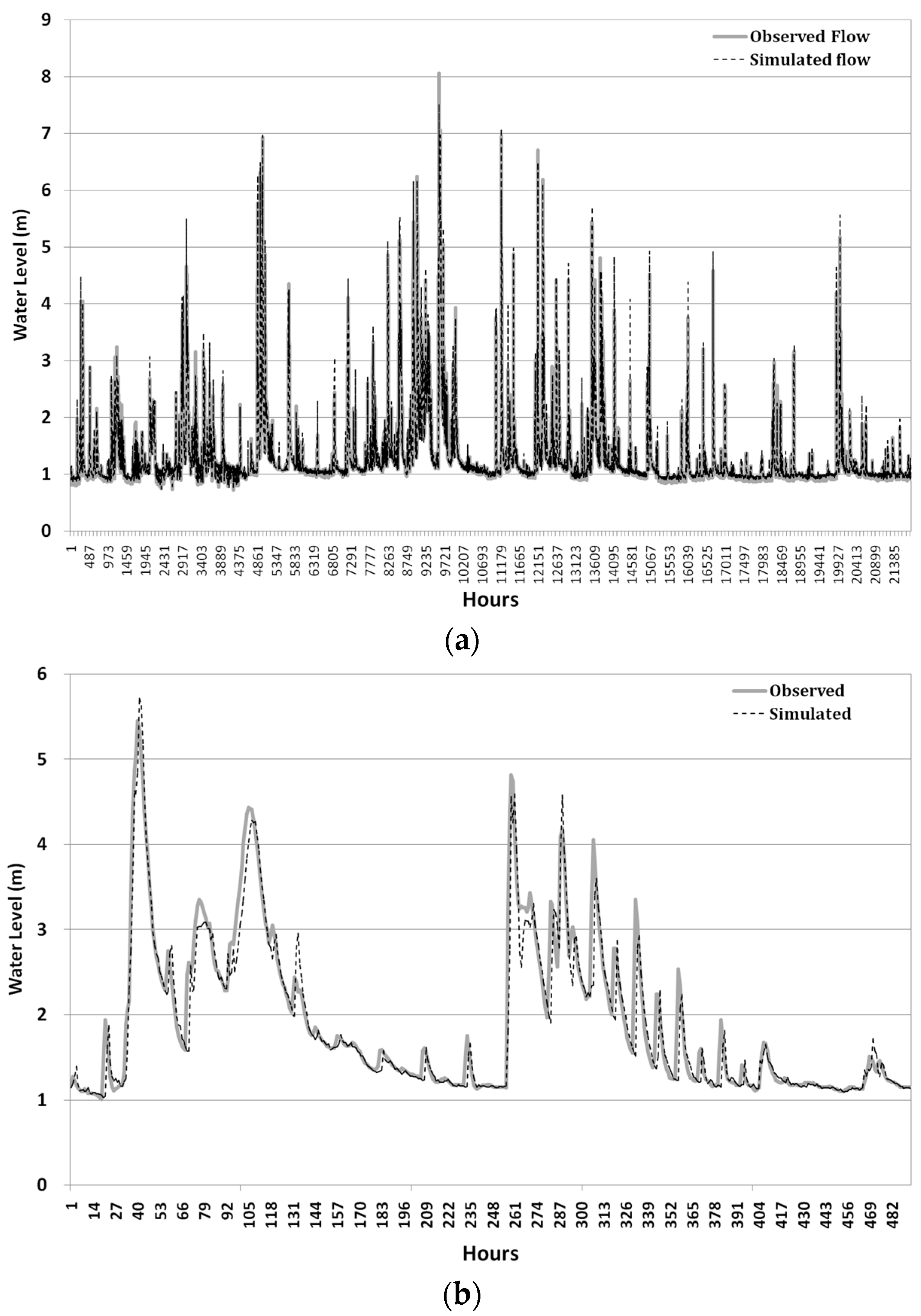
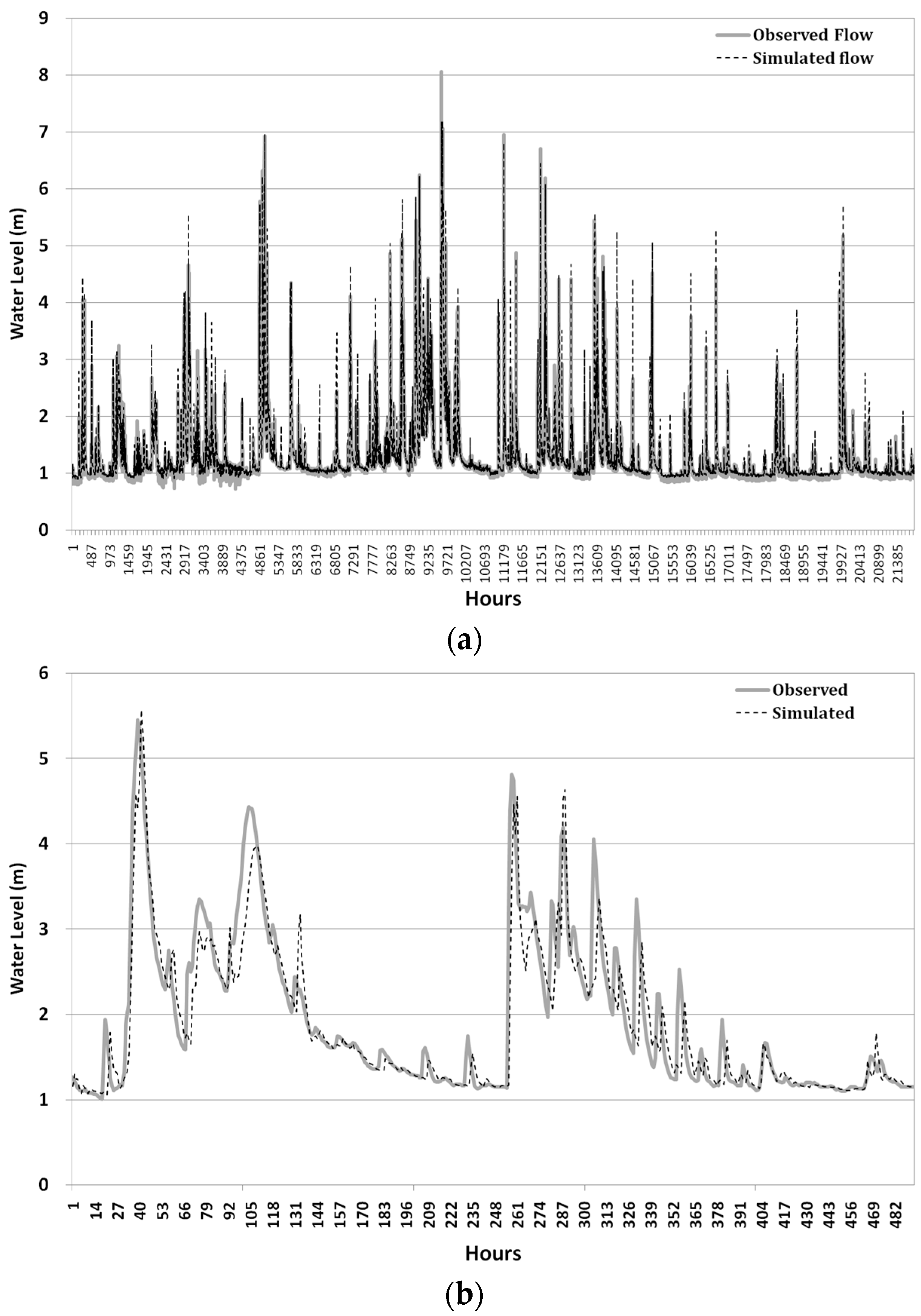
The observed and forecasted hourly water level series during training and testing periods from the best ANN model, ANN1d, were compared, as shown in Figure 10a,b focuses on of the flood period in test years and the forecasted water levels with 1 h of lead-time, which matched with observations.
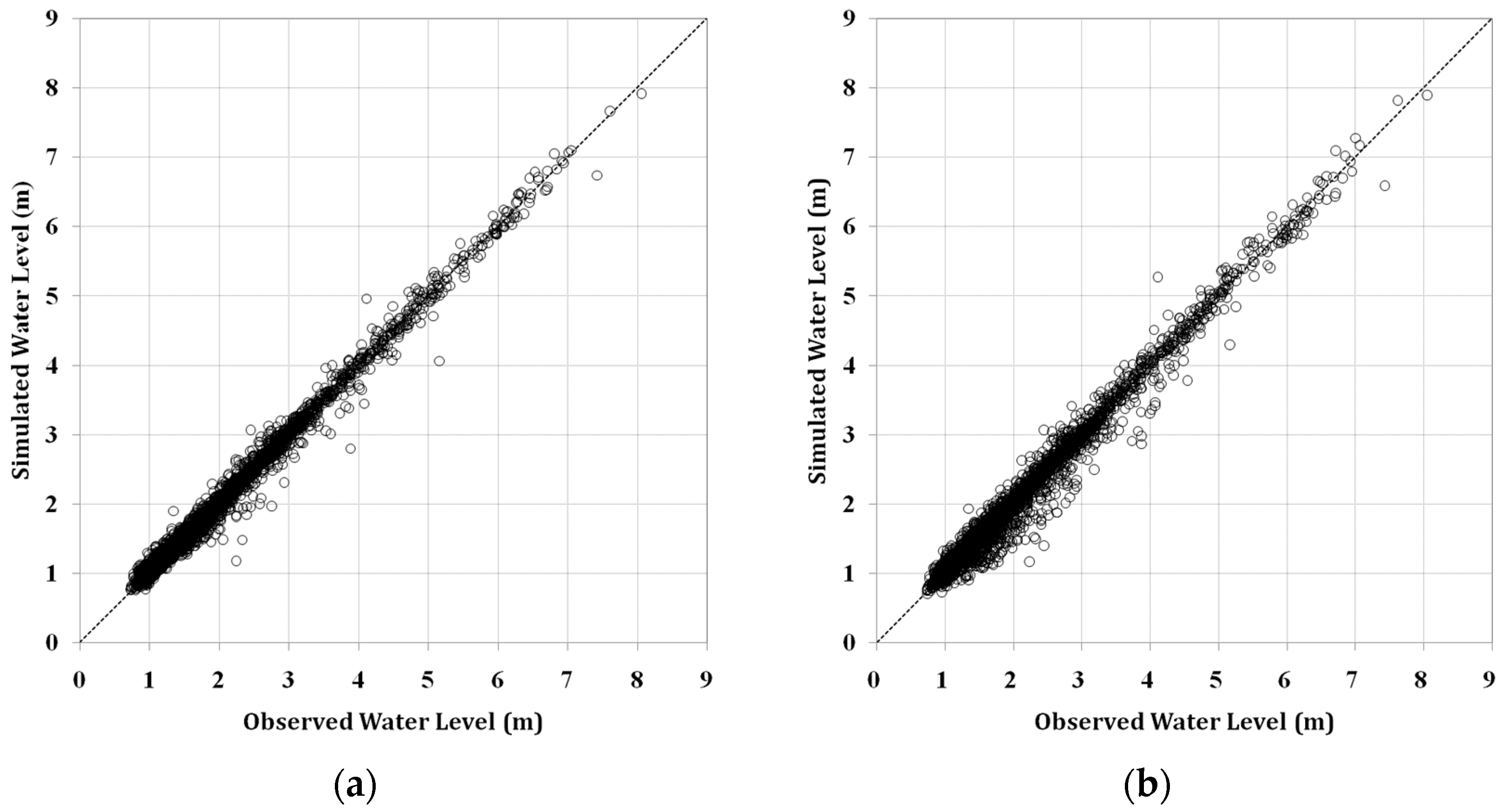
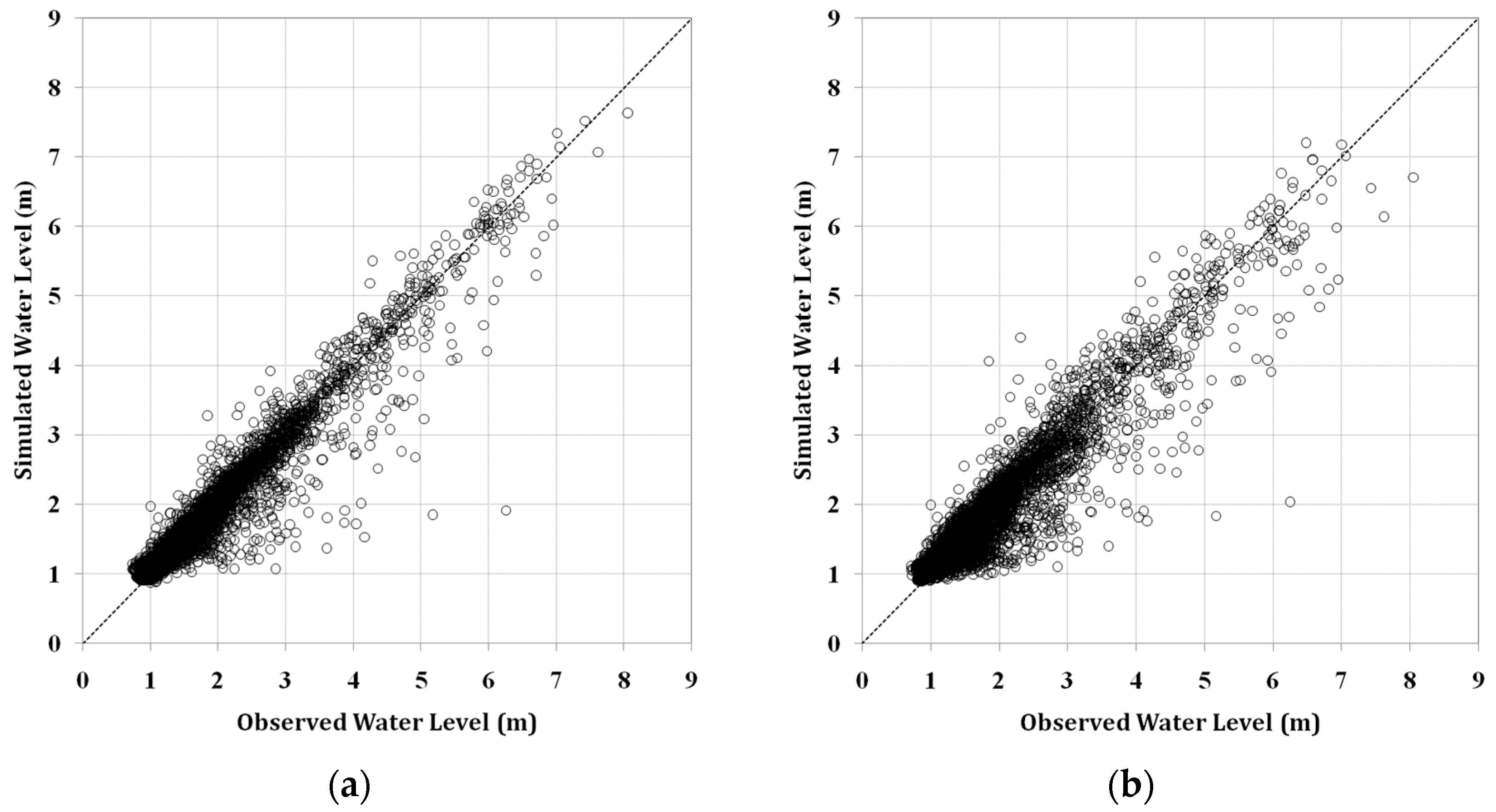
A scatter plot of observed and forecasted water levels from ANN1d during the training period is shown in Figure 11a. For comparative purpose, the results from ANN1a, in which upstream and downstream data were not included in the input vector, are shown in Figure 11b. Overall, it was evident that for 1 h lead-time of forecasting, ANN1d provided more accurate forecasting results than ANN1a.
3.3. Performance of ANN Models for 2 h Lead-Time Forecasting
The statistical measurements of four ANN models for 2 h lead-time forecasting are given in Table 6. These four models showed fairly good forecasting performance with NSE above 0.920, R2 above 0.920, and RMSE below 0.152 m using all water level data from both training and testing data sets. The best ANN model for 2 h lead-time forecasting using training (testing) data sets was ANN2d, which had the lowest RMSE value, at 0.1132 m (0.0936 m); the highest NSE, at 0.9754 (0.9533); and the highest R2, at 0.9758 (0.9542). Consistent good model performance was found for all water level data sets (Table 6).
As given in Table 7, when only the 5% highest water level data were used, the models also showed satisfactory performance. However, linear correlation was reduced for the testing data set. When ANN2a and ANN2b models were compared, the inclusion of upstream water level data as an input vector did not yield an appreciable effect on the performance of 2 h lead-time forecasting, which is consistent with results for 1 h lead-time forecasting.
Figure 12 shows a comparison of observed and forecasted water level data using the best ANN model, ANN2d, with a 2 h lead-time. It is obvious that the forecasted water levels are acceptable for 2 h of lead-time.
Scatter plots of observed and forecasted output water levels from ANN2d and ANN2a models are shown in Figure 13a,b, respectively. When forecasting 2 h ahead in time, the output data of ANN2d were less scattered compared with those of ANN2a. This result indicates that the use of additional water level data from multiple stations to networks clearly reduced error to a greater degree than that when only water level data was used from the station of interest. A comparison of Figure 11 and Figure 13 revealed that although the dispersion of points increased from 1 h ahead forecasting to 2 h ahead forecasting, it remained satisfactory. Interestingly, the underestimated points increased for the case of 2 h forecasting, which might have been caused by a lack of rainfall information. That is, ANN models for the study area based on current and previous rainfall data only, without considering future anticipated rainfall data, could not sufficiently represent the abruptly rising phenomena in stream flow hydrographs with a time of concentration of 1 to 2 h for the study catchment.
3.4. Performance of ANN Models for 3 h Lead-Time Forecasting
The performances of the four ANN models for 3 h ahead water level forecasting are given in Table 8. As expected, when the lead-time was increased from 1 to 3 h, the performances of all models decreased, and less accurate forecast values were obtained. ANN3c and ANN3d models provided more accurate forecasts than the other two models. The best model was ANN3c, which had an RMSE of 0.1716 (0.1421), NSE of 0.9403 (0.8844), and R2 of 0.9443 (0.8941) for the training (testing) data set.
Statistical measures for the 5% highest water level forecasts with a lead-time of 3 h are given in Table 9. Similarly, ANN3c and ANN3d presented significantly better results than the other two models. It is clear that the inclusion of water level data at the main river to the network improved the model performance for forecasting with a lead-time of 3 h. However, these models appeared to produce considerable error for high flow prediction. In particular, the reduced NSE and R2 values for the testing data set revealed that considerable differences can occur between the forecasted and observed water levels. To increase the accuracy for longer lead-times, other input variables that could affect stream-flow, such as forecasted rainfall data, need to be included in the network model.
A comparison of hydrographs between observed and forecasted water levels with a 3 h lead-time from the best model, ANN3c, is shown in Figure 14. Overall, under- and over estimations were observed. As shown in the figure, the trend of forecasted water levels might be acceptable; however, the forecasting results contained many errors. Moreover, time shifts were found for some peaks and rising parts between observations and forecasts, as shown in Figure 14b.
Figure 15a presents a plot between observed and forecasted water levels with a lead-time of 3 h using ANN3c, the best model; Figure 15b shows the results from ANN3a. ANN3c was insufficient for predicting the water level with a lead-time of 3 h even though the use of multiple water level data clearly improved the model performance. Moreover, the forecasted values from the ANN3c model were underestimated at many points, which is similar to the results for forecasting with a lead-time of 2 h. As described above, the rainfall data used for ANN models in this study were not sufficient for forecasting the water level with a lead-time of 3 h for a study area with a short time of concentration.
4. Conclusions
Since urban floods frequently occur in tributaries of the Han River, South Korea, in which flood water level rises due to the backwater effect, accurate and efficient methodology to predict water levels is very important in producing countermeasures against flood disasters. For this purpose, artificial neural network models were developed in this study to forecast hourly water levels on a tributary where the influence of hydrologic boundary conditions at a downstream confluence was apparent. The main points of this research are given below.
(1) ANN models were constructed for forecasting water levels with lead-times of 1–3h by using the input data, areal average rainfall, water level data at the station of interest, water level data at an upstream gauging station, and water level data at multiple stations located near the confluence of the tributary, Anyangcheon stream, and the main river, the Han River.
(2) The proposed ANN models were capable of forecasting water levels with high accuracy up to a 2 h lead-time based on the statistical measures of RSME, R2, and NSE. However, the models showed unsatisfactory performance in forecasting with a 3 h lead-time.
(3) The proposed ANN models improved the accuracy of forecasting water levels by including the water level of the main river gauging station as input data. Therefore, the ANN models can simulate accurate water level forecasts considering the backwater effect without the use of complex physical models.
Author Contributions
All authors substantially contributed in conceiving and designing of the approach and realizing this manuscript. Ji Youn Sung and Jeongwoo Lee prepared the input data and implemented the artificial neural network models. Ji Youn Sung, Jeongwoo Lee, and Il-Moon Chung worked on the analysis and presentation of the results. Jun-Haeng Heo supervised the entire research. All four authors jointly wrote the paper. All authors have read and approved the final manuscript.
Conflicts of Interest
The authors declare no conflict of interest.
References
- Hapuarachchi, H.A.P.; Wang, Q.J.; Pagano, T.C. A review of advances in flash flood forecasting. Hydrol. Process. 2011, 25, 2771–2784. [Google Scholar] [CrossRef]
- ASCE Task Committee on Application of Artificial Neural Networks in Hydrology. Artificial neural networks in hydrology. I: Preliminary concepts. J. Hydrol. Eng. 2000, 5, 115–123. [Google Scholar]
- Kumar, A.P.S.; Sudheer, K.P.; Jain, S.K.; Agarwal, P.K. Rainfall runoff modeling using artificial neural networks: Comparison of network types. Hydrol. Process. 2005, 19, 1277–1291. [Google Scholar] [CrossRef]
- Tokar, A.S.; Johnson, A. Rainfall-runoff modeling using artificial neural networks. J. Hydrol. Eng. 1999, 4, 232–239. [Google Scholar] [CrossRef]
- Tokar, A.S.; Markus, M. Precipitation-runoff modeling using artificial neural networks and conceptual models. J. Hydrol. Eng. 2000, 5, 156–161. [Google Scholar] [CrossRef]
- Yu, P.S.; Chen, S.T.; Chang, I.F. Support vector regression for real-time flood stage forecasting. J. Hydrol. 2006, 328, 704–716. [Google Scholar] [CrossRef]
- Thimuralaiah, K.; Deo, M.C. Hydrological forecasting using neural networks. J. Hydrol. Eng. 2000, 5, 180–189. [Google Scholar]
- Napolitano, G.; Seeb, L.; Calvo, B.; Savi, F.; Heppenstall, A. A conceptual and neural network model for real-time flood forecastingof the Tiber River in Rome. Phys. Chem. Earth 2010, 35, 187–194. [Google Scholar] [CrossRef]
- Bertoni, J.C.; Tucci, C.E.; Clarke, R.T. Rainfall-based real-time flood forecasting. J. Hydrol. 1992, 131, 313–339. [Google Scholar] [CrossRef]
- Bonafe, A.; Galeati, G.; Sforna, M. Neural networks for daily mean flow forecasting. Trans. Ecol. Environ. 1994, 7, 131–138. [Google Scholar]
- Karunanithi, N.; Grenney, W.J.; Whitley, D.; Bovee, K. Neural networks for river flow prediction. J. Comput. Civ. Eng. 1994, 8, 201–220. [Google Scholar] [CrossRef]
- Shamseldin, A.Y.; O’Connor, K.M. A real-time combination method for the outputs of different rainfall–runoff models. Hydrol. Sci. J. 1999, 44, 895–912. [Google Scholar] [CrossRef]
- Georgakakos, K.P.; Seo, D.J.; Gupta, H.; Schaake, J.; Butts, M.B. Towards the characterization of stream-flow simulation uncertainty through multi-model ensembles. J. Hydrol. 2004, 298, 222–241. [Google Scholar] [CrossRef]
- Young, C.C.; Liu, W.C. Prediction and modelling of rainfall–runoff during typhoon events using a physically-based and artificial neural network hybrid model. Hydrol. Sci. J. 2015, 60, 2102–2116. [Google Scholar] [CrossRef]
- Atiya, A.F.; Samir, I. A comparison between neural-network forecasting techniques—Case study: River flow forecasting. Trans. Neural Netw. 1999, 10, 402–409. [Google Scholar] [CrossRef]
- Dawson, C.W.; Wilby, R.L. Hydrological modeling using artificial neural networks. Prog. Phys. Geogr. 2001, 25, 80–108. [Google Scholar] [CrossRef]
- Yaseen, Z.M.; Ahmed, E.S.; Afan, H.A.; Hameed, M.; Mohtar, W.H.M.W.; Hussain, A. RBFNN versus FFNN for daily river flow forecasting at Johor River, Malaysia. Neural Comput. Appl. 2016, 27, 1533–1542. [Google Scholar] [CrossRef]
- Chang, L.C.; Chang, F.J.; Chiang, Y.M. A two-step-ahead recurrent neural network for stream-flow forecasting. Hydol. Process. 2004, 18, 81–92. [Google Scholar] [CrossRef]
- Elsafi, H.S. Artificial Neural Networks (ANNs) for flood forecasting at Dongola Station in the River Nile, Sudan. Alex. Eng. J. 2014, 53, 655–662. [Google Scholar] [CrossRef]
- Chang, F.J.; Chen, P.A.; Lu, Y.R.; Huang, E.; Chang, K.Y. Real-time multi-step-ahead water level forecasting by recurrent neural networks for urban flood control. J. Hydrol. 2014, 517, 836–846. [Google Scholar] [CrossRef]
- Latt, Z.Z.; Wittenberg, H. Improving flood forecasting in a developing country: A comparative study of stepwise multiple linear regression and artificial neural network. Water Resour. Manag. 2014, 28, 2109–2128. [Google Scholar] [CrossRef]
- Aichouri, I.; Hani, A.; Bougherira, N.; Djabri, L.; Chaffai, H.; Lallahem, S. River flow model using artificial neural networks. Energy Procedia 2015, 74, 1007–1014. [Google Scholar] [CrossRef]
- Todini, E. Role and treatment of uncertainty in real-time flood forecasting. Hydrol. Process. 2004, 18, 2743–2746. [Google Scholar] [CrossRef]
- Badrzadeh, H.; Sarukkalige, R.; Jayawardena, A.W. Hourly runoff forecasting for flood risk management: Application of various computational intelligence models. J. Hydrol. 2015, 529, 1633–1643. [Google Scholar] [CrossRef]
- Tiwari, M.K.; Chatterjee, C. Development of an accurate and reliable hourly flood forecasting model using wavelet-bootstrap-ANN (WBANN) hybrid approach. J. Hydrol. 2010, 394, 458–470. [Google Scholar] [CrossRef]
- Lizhen, L.; Yu, J.; Zhang, S.; Zhou, H. Short-term water level prediction using differentartificial intelligent models. In Proceedings of the 2016 5th International Conference on Agro-geoinformatics, Tianjin, China, 18–20 July 2016. [Google Scholar] [CrossRef]
- Luan, Q.; Cheng, Y.; Ima, Z. Test on flood prediction-model using artificial neural network for ShiiLiAn hydrologic station on MinChiang, China. Appl. Mech. Mater. 2011, 39, 555–561. [Google Scholar] [CrossRef]
- Christina, W. Flood routing in mild-sloped rivers–wave characteristics and downstream backwater effect. J. Hydrol. 2005, 308, 151–167. [Google Scholar]
- McCulloch, W.S.; Pitts, W. A logical calculus of the ideas immanent in nervous activity. Bull. Math. Biophys. 1943, 5, 115–133. [Google Scholar] [CrossRef]
- Adamowski, J.; Sun, K. Development of a coupled wavelet transform and neural network method for flow forecasting of non-perennial rivers in semi-arid watersheds. J. Hydrol. 2010, 390, 85–91. [Google Scholar] [CrossRef]
- Kim, T.W.; Valdes, J.B. Nonlinear model for drought forecasting based on a conjunction of wavelet transforms and neural networks. J. Hydrol. Eng. 2003, 8, 319–328. [Google Scholar] [CrossRef]
- Rumelhart, D.E.; McClenlland, J.L. Parallel Distributed Processing: Explorations in the Microstructure of Cognition, Vol. 1: Foundations; MIT Press: Cambridge, MA, USA, 1986. [Google Scholar]
- Supharatid, S. Application of a neural network model in establishing a stage-discharge relationship for a tidal river. Hydrol. Process. 2003, 17, 3085–3099. [Google Scholar] [CrossRef]
- Sudheer, K.P.; Jain, S.K. Radial basis function neural network for modeling rating curves. J. Hydrol. Eng. 2013, 8, 161–164. [Google Scholar] [CrossRef]
- Liang, S.X.; Li, M.C.; Sun, Z.C. Prediction models for tidal level including strong meteorologic effects using a neural network. Ocean Eng. 2008, 35, 666–675. [Google Scholar] [CrossRef]
Figure 1.
Anyangcheon stream.

Figure 2.
Study area showing Anyangcheon stream watershed and the Han River.

Figure 3.
Model construction cases with simple diagram.

Figure 4.
Concept of multilayer perceptron.
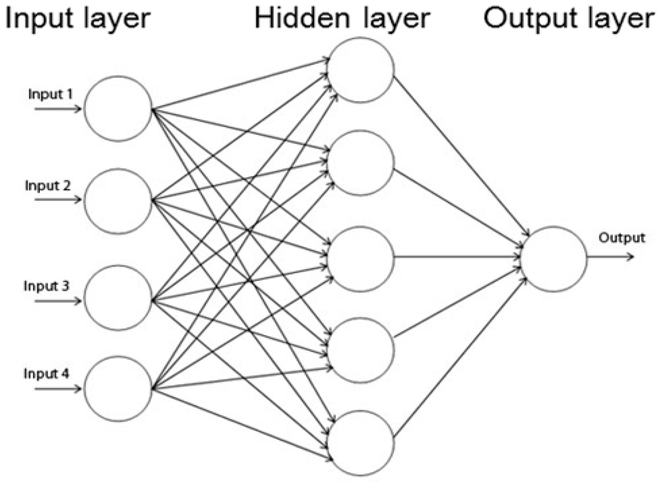
Figure 5.
Cross-correlation between water level at Ogeumgyo station (OG) and averaged rainfall series.
Figure 5.
Cross-correlation between water level at Ogeumgyo station (OG) and averaged rainfall series.
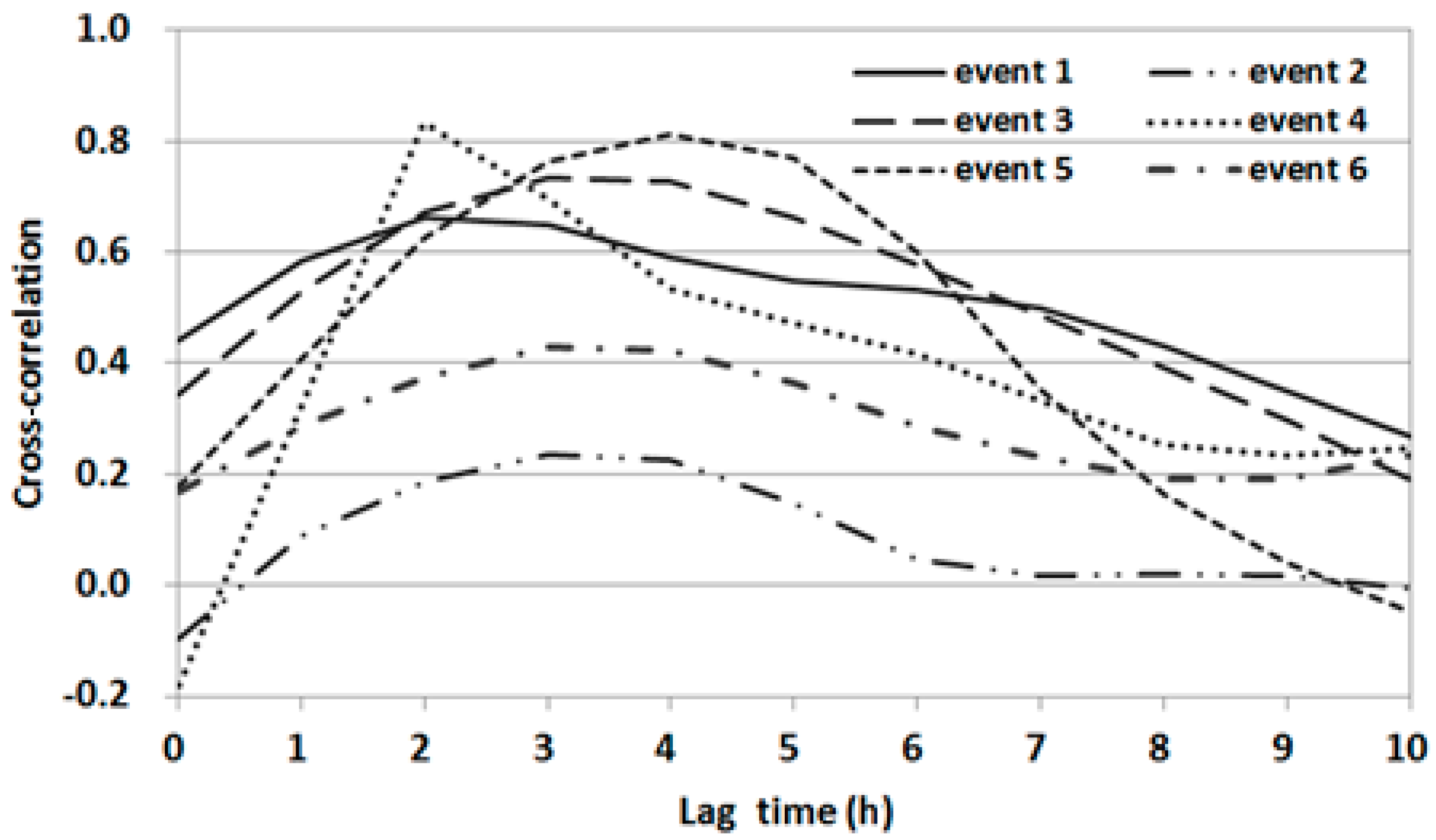
Figure 6.
Cross-correlation of water level series between Chunghungyo (CH) and OG.

Figure 7.
Cross-correlation of water level series between Hangangdaegyo (HG) and OG.
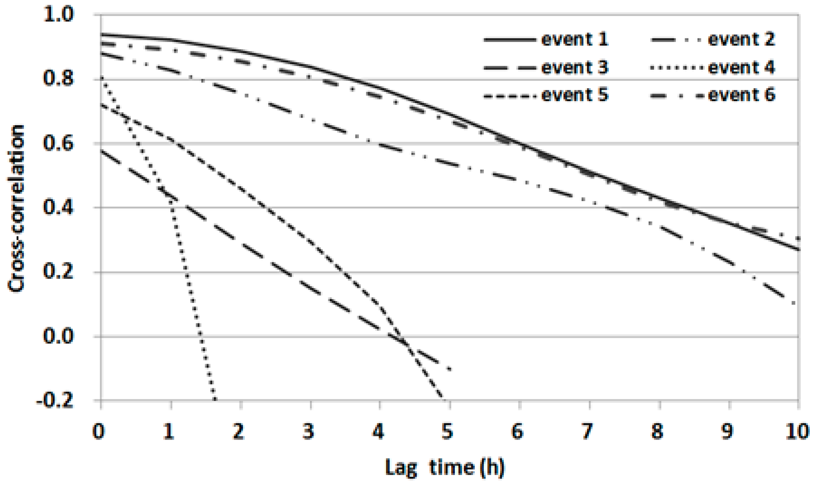
Figure 8.
Auto-correlation of water level series at OG.
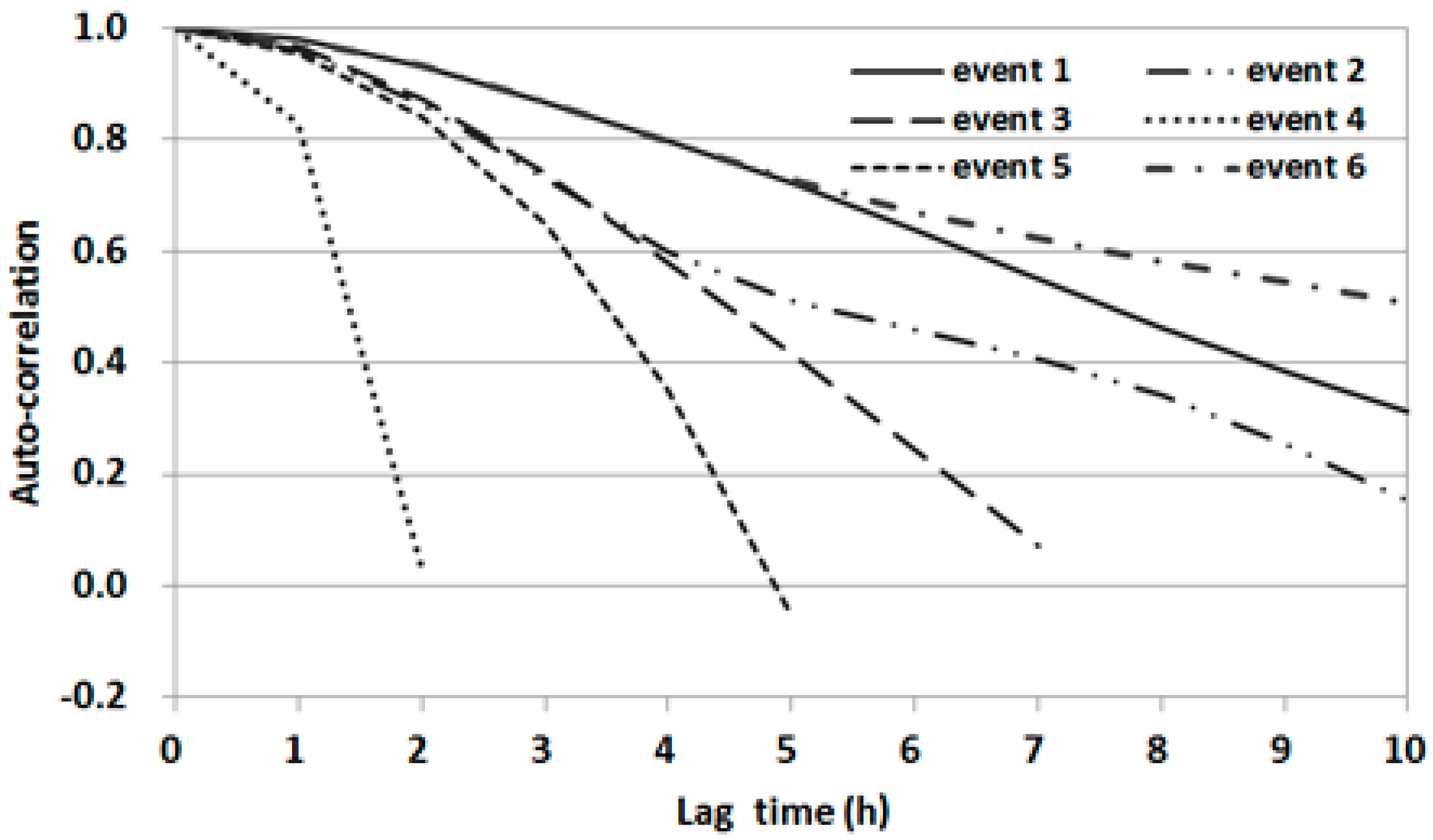
Figure 9.
Root mean square error (RMSE) of ANN1a and ANN3c models according to the number of hidden nodes and previous time span. (a) ANN1a; (b) ANN3c.
Figure 9.
Root mean square error (RMSE) of ANN1a and ANN3c models according to the number of hidden nodes and previous time span. (a) ANN1a; (b) ANN3c.
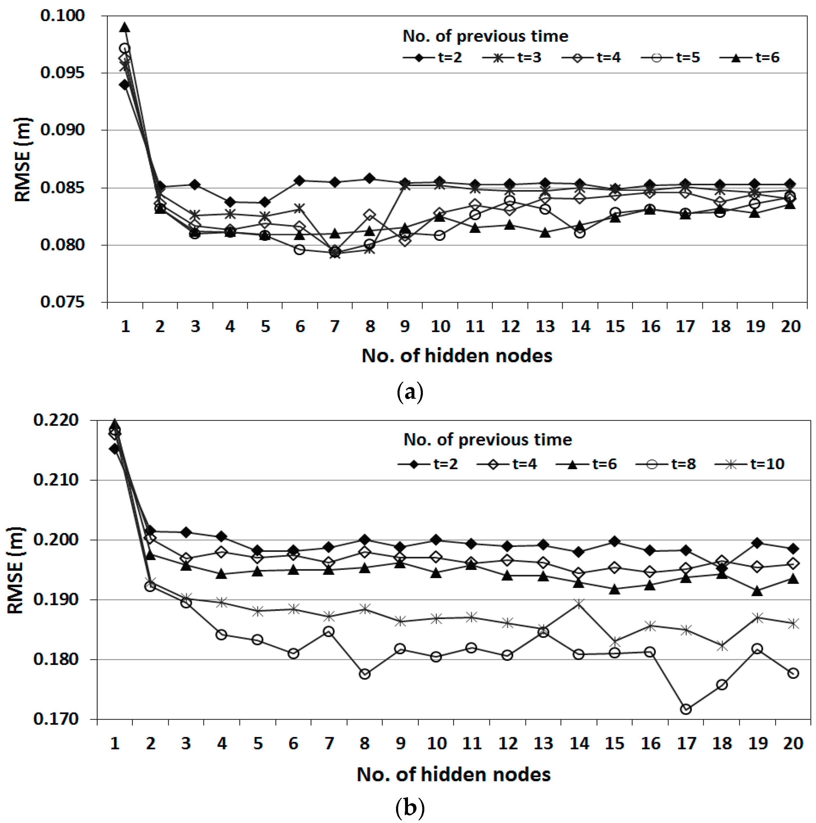
Figure 10.
Comparison of observed and forecasted water levels with a lead-time of 1 h. (a) Water level of training and test periods; (b) Water level of some period in testing data set.
Figure 10.
Comparison of observed and forecasted water levels with a lead-time of 1 h. (a) Water level of training and test periods; (b) Water level of some period in testing data set.
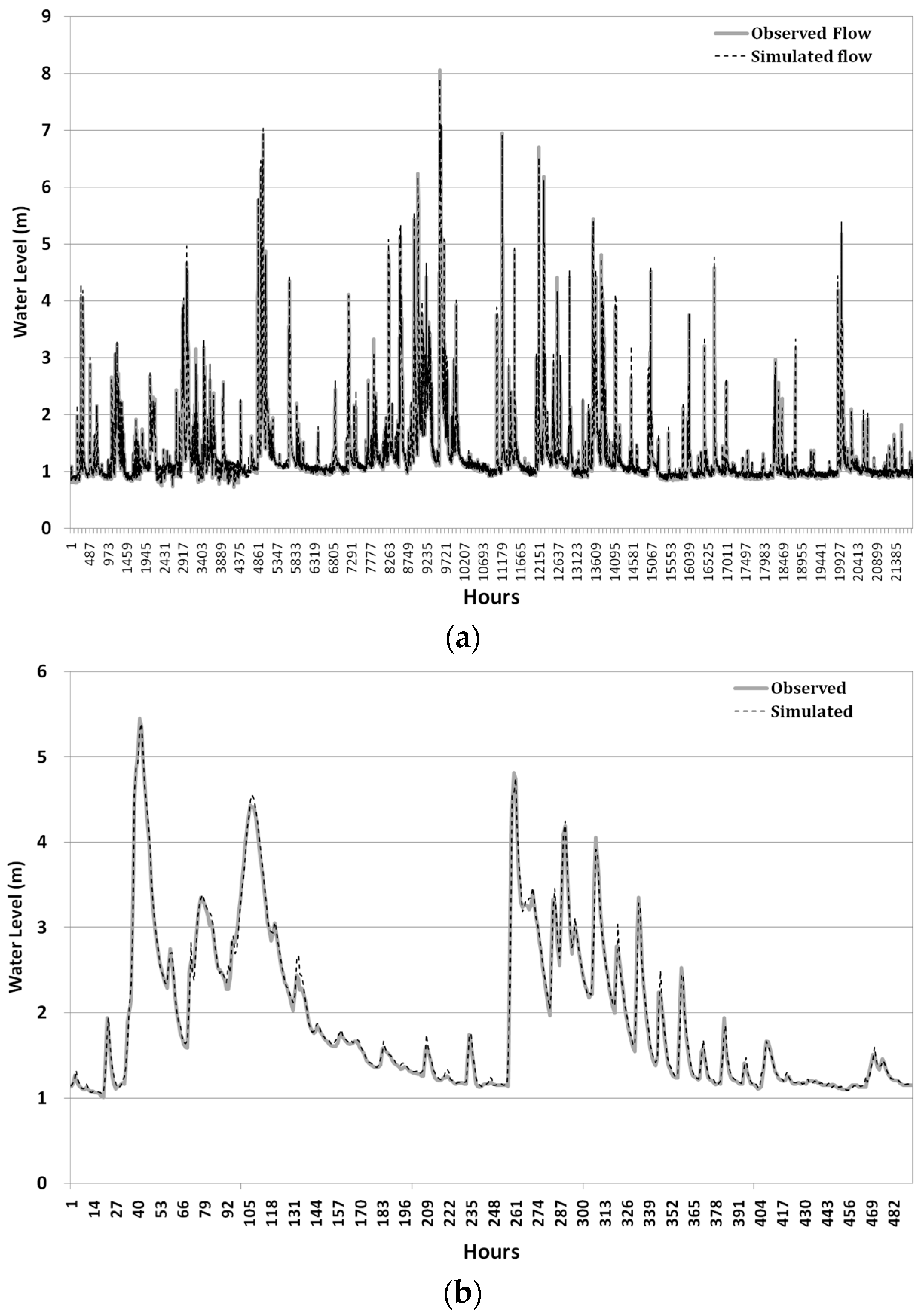
Figure 11.
Scatter plots of observed and forecasted water levels with a lead-time of 1 h. (a) ANN1d; (b) ANN1a.
Figure 11.
Scatter plots of observed and forecasted water levels with a lead-time of 1 h. (a) ANN1d; (b) ANN1a.

Figure 12.
Comparison of observed and forecasted water levels with a lead-time of 2h. (a) Water level of training and testing periods; (b) Water level of some period in testing data set.
Figure 12.
Comparison of observed and forecasted water levels with a lead-time of 2h. (a) Water level of training and testing periods; (b) Water level of some period in testing data set.

Figure 13.
Scatter plots of observed and forecasted water levels with a lead-time of 2 h. (a) ANN2d; (b) ANN2a.
Figure 13.
Scatter plots of observed and forecasted water levels with a lead-time of 2 h. (a) ANN2d; (b) ANN2a.
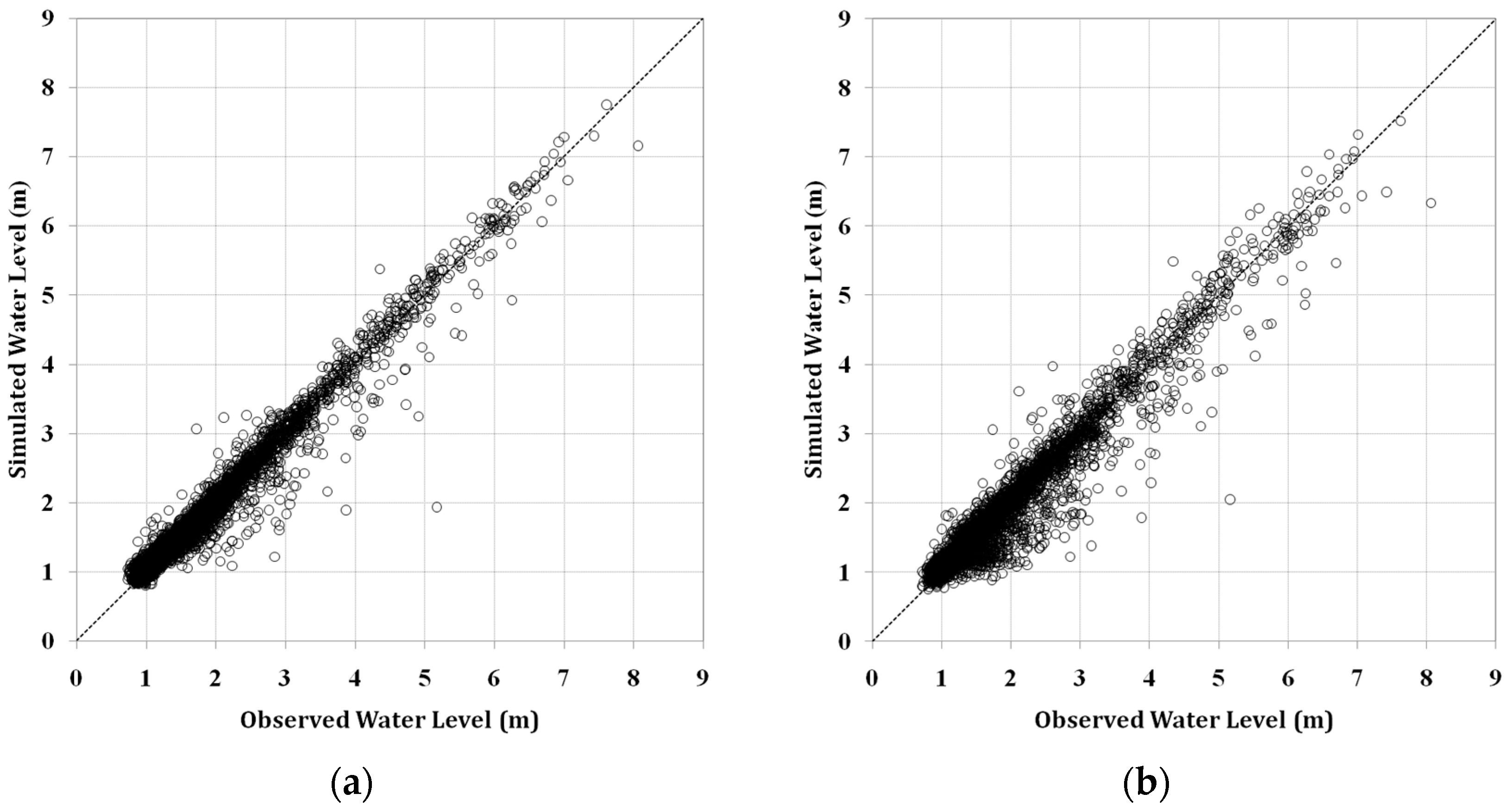
Figure 14.
Comparison of observed and forecasted water levels with a lead-time of 3 h. (a) Water level of training and testing periods; (b) Water level of some period in testing data set.
Figure 14.
Comparison of observed and forecasted water levels with a lead-time of 3 h. (a) Water level of training and testing periods; (b) Water level of some period in testing data set.

Figure 15.
Scatter plots of observed and forecasted water levels with a lead-time of 3 h. (a) ANN3c; (b) ANN3a.
Figure 15.
Scatter plots of observed and forecasted water levels with a lead-time of 3 h. (a) ANN3c; (b) ANN3a.


Table 1.
Selected flood events for correlation analysis.
| Event Number | Event Period | Peak Water Level (El.m) |
|---|---|---|
| 1 | 19:00 07/13 to 22:00 07/16/2009 | 6.93 |
| 2 | 16:00 07/26 to 03:00 07/29/2011 | 8.06 |
| 3 | 13:00 07/05 to 19:00 07/06/2012 | 6.95 |
| 4 | 11:00 08/15 to 17:00 08/15/2012 | 6.71 |
| 5 | 20:00 07/12 to 11:00 07/13/2013 | 5.45 |
| 6 | 09:00 07/04 to 00:00 07/06/2016 | 5.18 |
Table 2.
Four groups of artificial neural network models with input variables (model configuration).
Table 2.
Four groups of artificial neural network models with input variables (model configuration).
| Models | Input Variable | Output Variable |
|---|---|---|
| ANNia | ||
| ANNib | ||
| ANNic | ||
| ANNid | ||
Table 3.
Optimal configuration of ANN models.
| Model | Leadtime (i) | Previous Time (τ) | Number of Hidden Nodes (h) |
|---|---|---|---|
| (h) | (h) | (EA) | |
| ANNia | 1 | 3 | 7 |
| 2 | 4 | 10 | |
| 3 | 8 | 6 | |
| ANNib | 1 | 3 | 11 |
| 2 | 9 | 16 | |
| 3 | 10 | 18 | |
| ANNic | 1 | 5 | 16 |
| 2 | 8 | 17 | |
| 3 | 8 | 17 | |
| ANNid | 1 | 7 | 12 |
| 2 | 10 | 20 | |
| 3 | 10 | 19 |
Table 4.
Statistical measurement of 1 h forecasts for the entire data set.
| Model | Training | Testing | ||||
|---|---|---|---|---|---|---|
| RMSE | NSE | R2 | RMSE | NSE | R2 | |
| ANN1a | 0.0793 | 0.9879 | 0.9881 | 0.0630 | 0.9781 | 0.9792 |
| ANN1b | 0.0757 | 0.9890 | 0.9892 | 0.0606 | 0.9796 | 0.9804 |
| ANN1c | 0.0595 | 0.9932 | 0.9933 | 0.0510 | 0.9858 | 0.9862 |
| ANN1d | 0.0585 | 0.9935 | 0.9936 | 0.0502 | 0.9864 | 0.9868 |
Table 5.
Statistical measurement of 1 h forecasts for 5% highest water level data.
| Model | Training | Testing | ||||
|---|---|---|---|---|---|---|
| RMSE | NSE | R2 | RMSE | NSE | R2 | |
| ANN1a | 0.1166 | 0.9936 | 0.9937 | 0.1113 | 0.9511 | 0.9500 |
| ANN1b | 0.1064 | 0.9947 | 0.9948 | 0.1078 | 0.9553 | 0.9541 |
| ANN1c | 0.0865 | 0.9965 | 0.9965 | 0.0876 | 0.9705 | 0.9700 |
| ANN1d | 0.0869 | 0.9964 | 0.9965 | 0.0819 | 0.9737 | 0.9735 |
Table 6.
Statistical measurement of 2 h forecasts for the entire data set.
| Model | Training | Testing | ||||
|---|---|---|---|---|---|---|
| RMSE | NSE | R2 | RMSE | NSE | R2 | |
| ANN2a | 0.1519 | 0.9543 | 0.9563 | 0.1161 | 0.9222 | 0.9292 |
| ANN2b | 0.1458 | 0.9583 | 0.9598 | 0.1124 | 0.9267 | 0.9327 |
| ANN2c | 0.1156 | 0.9740 | 0.9747 | 0.0955 | 0.9494 | 0.9517 |
| ANN2d | 0.1132 | 0.9754 | 0.9758 | 0.0936 | 0.9533 | 0.9542 |
Table 7.
Statistical measures of 2 h forecasts for 5% highest water level data.
| Model | Training | Testing | ||||
|---|---|---|---|---|---|---|
| RMSE | NSE | R2 | RMSE | NSE | R2 | |
| ANN2a | 0.2654 | 0.9650 | 0.9686 | 0.2100 | 0.8429 | 0.8334 |
| ANN2b | 0.2554 | 0.9680 | 0.9706 | 0.2065 | 0.8500 | 0.8401 |
| ANN2c | 0.2103 | 0.9786 | 0.9798 | 0.1680 | 0.8998 | 0.8947 |
| ANN2d | 0.2070 | 0.9796 | 0.9804 | 0.1660 | 0.9030 | 0.9000 |
Table 8.
Statistical measurement of 3 h forecasts for the entire data set.
| Model | Training | Testing | ||||
|---|---|---|---|---|---|---|
| RMSE | NSE | R2 | RMSE | NSE | R2 | |
| ANN3a | 0.2108 | 0.9091 | 0.9159 | 0.1611 | 0.8472 | 0.8635 |
| ANN3b | 0.2046 | 0.9149 | 0.9208 | 0.1528 | 0.8582 | 0.8745 |
| ANN3c | 0.1716 | 0.9403 | 0.9443 | 0.1421 | 0.8844 | 0.8941 |
| ANN3d | 0.1723 | 0.9398 | 0.9438 | 0.1462 | 0.8792 | 0.8952 |
Table 9.
Statistical measurement of 3 h forecasts for top 5% high water level data.
| Model | Training | Testing | ||||
|---|---|---|---|---|---|---|
| RMSE | NSE | R2 | RMSE | NSE | R2 | |
| ANN3a | 0.4028 | 0.9124 | 0.9301 | 0.2943 | 0.7105 | 0.6881 |
| ANN3b | 0.3995 | 0.914 | 0.9313 | 0.2989 | 0.7142 | 0.6870 |
| ANN3c | 0.3359 | 0.9422 | 0.9503 | 0.2663 | 0.7768 | 0.7561 |
| ANN3d | 0.3366 | 0.9425 | 0.9501 | 0.2637 | 0.7747 | 0.7586 |
© 2017 by the authors. Licensee MDPI, Basel, Switzerland. This article is an open access article distributed under the terms and conditions of the Creative Commons Attribution (CC BY) license (http://creativecommons.org/licenses/by/4.0/).
Share and Cite
MDPI and ACS Style
Sung, J.Y.; Lee, J.; Chung, I.-M.; Heo, J.-H. Hourly Water Level Forecasting at Tributary Affected by Main River Condition. Water 2017, 9, 644. https://doi.org/10.3390/w9090644
AMA Style
Sung JY, Lee J, Chung I-M, Heo J-H. Hourly Water Level Forecasting at Tributary Affected by Main River Condition. Water. 2017; 9(9):644. https://doi.org/10.3390/w9090644
Chicago/Turabian StyleSung, Ji Youn, Jeongwoo Lee, Il-Moon Chung, and Jun-Haeng Heo. 2017. "Hourly Water Level Forecasting at Tributary Affected by Main River Condition" Water 9, no. 9: 644. https://doi.org/10.3390/w9090644
Note that from the first issue of 2016, this journal uses article numbers instead of page numbers. See further details here.