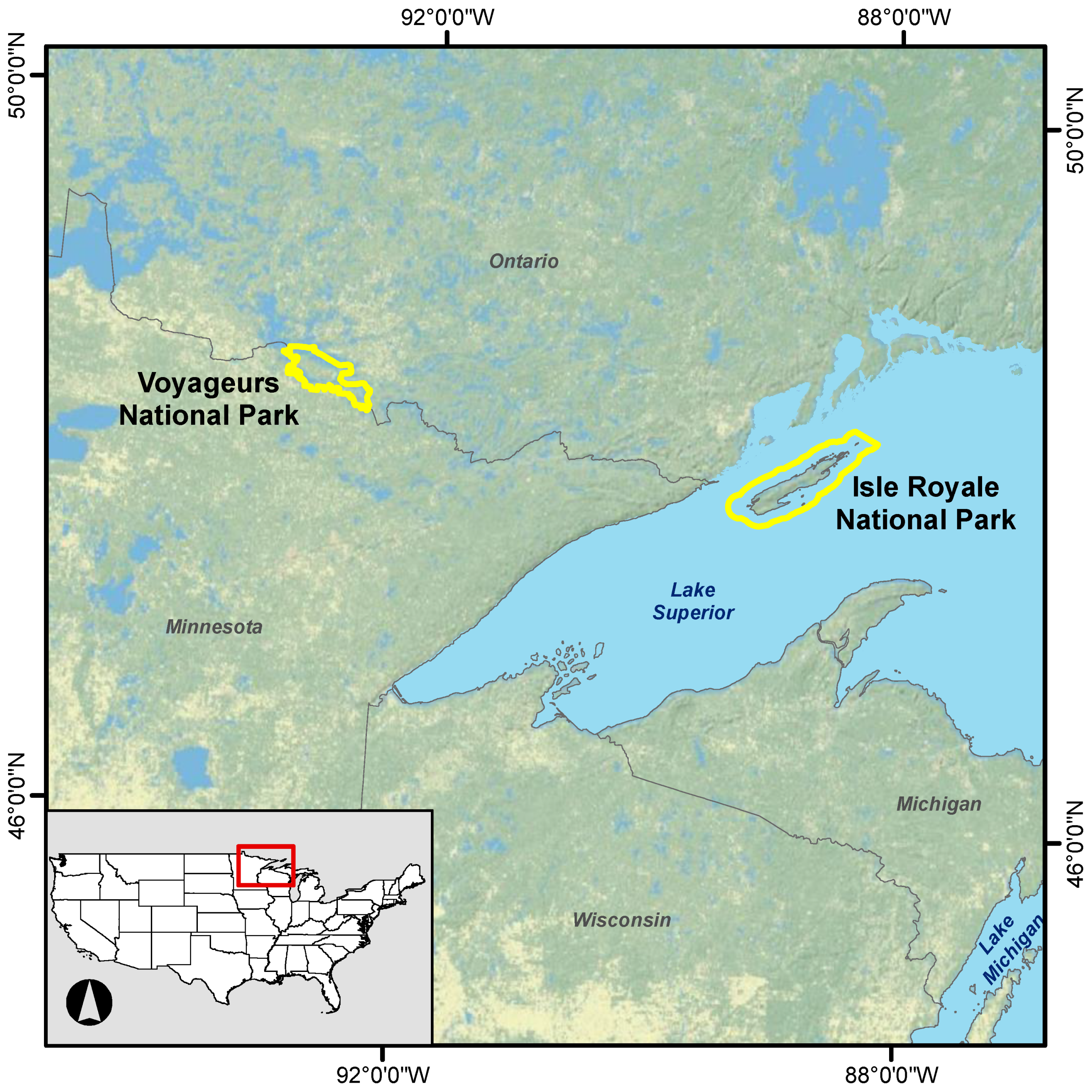
Figure 1.
Locations of Voyageurs and Isle Royale national parks.
Figure 1.
Locations of Voyageurs and Isle Royale national parks.
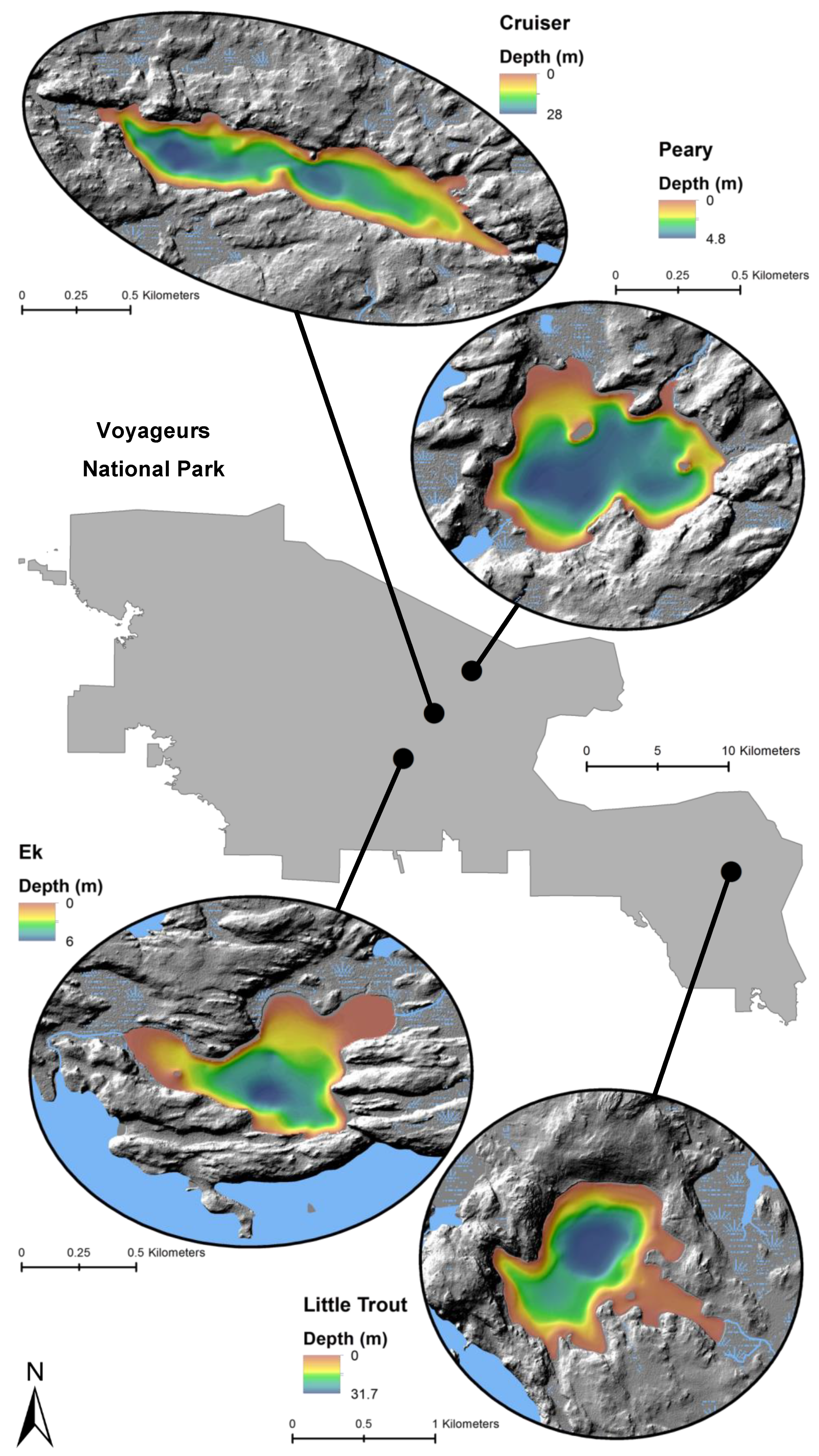
Figure 2.
Locations and bathymetry (m) of four study lakes within Voyageurs National Park.
Figure 2.
Locations and bathymetry (m) of four study lakes within Voyageurs National Park.
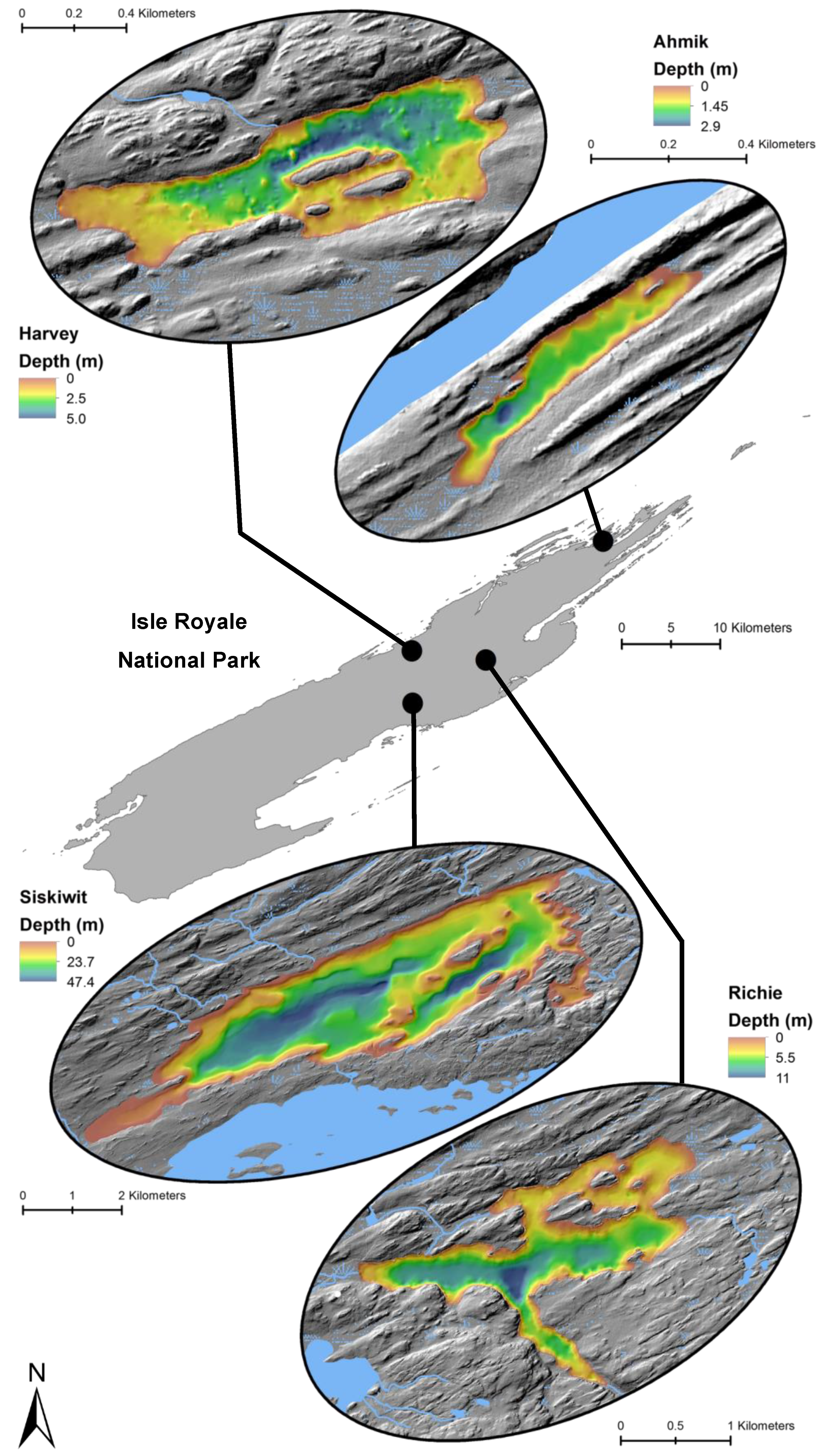
Figure 3.
Locations and bathymetry (m) of four study lakes within Isle Royale National Park.
Figure 3.
Locations and bathymetry (m) of four study lakes within Isle Royale National Park.
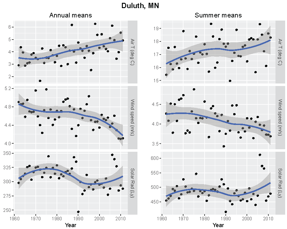
Figure 4.
Annual and summer weather patterns at Duluth, Minnesota, 1962–2011. Left panels are the annual means of air temperature (°C), wind speed (m/s), and solar radiation (Langley). Right panels are the summer means of the same parameters.
Figure 4.
Annual and summer weather patterns at Duluth, Minnesota, 1962–2011. Left panels are the annual means of air temperature (°C), wind speed (m/s), and solar radiation (Langley). Right panels are the summer means of the same parameters.
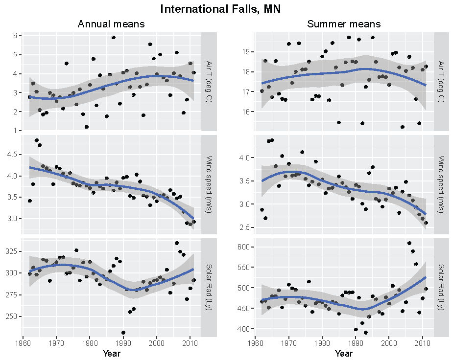
Figure 5.
Annual and summer weather patterns at International Falls, Minnesota, 1962–2011. Left panels are the annual means of air temperature (°C), wind speed (m/s), and solar radiation (Langley). Right panels are the summer means of the same parameters.
Figure 5.
Annual and summer weather patterns at International Falls, Minnesota, 1962–2011. Left panels are the annual means of air temperature (°C), wind speed (m/s), and solar radiation (Langley). Right panels are the summer means of the same parameters.
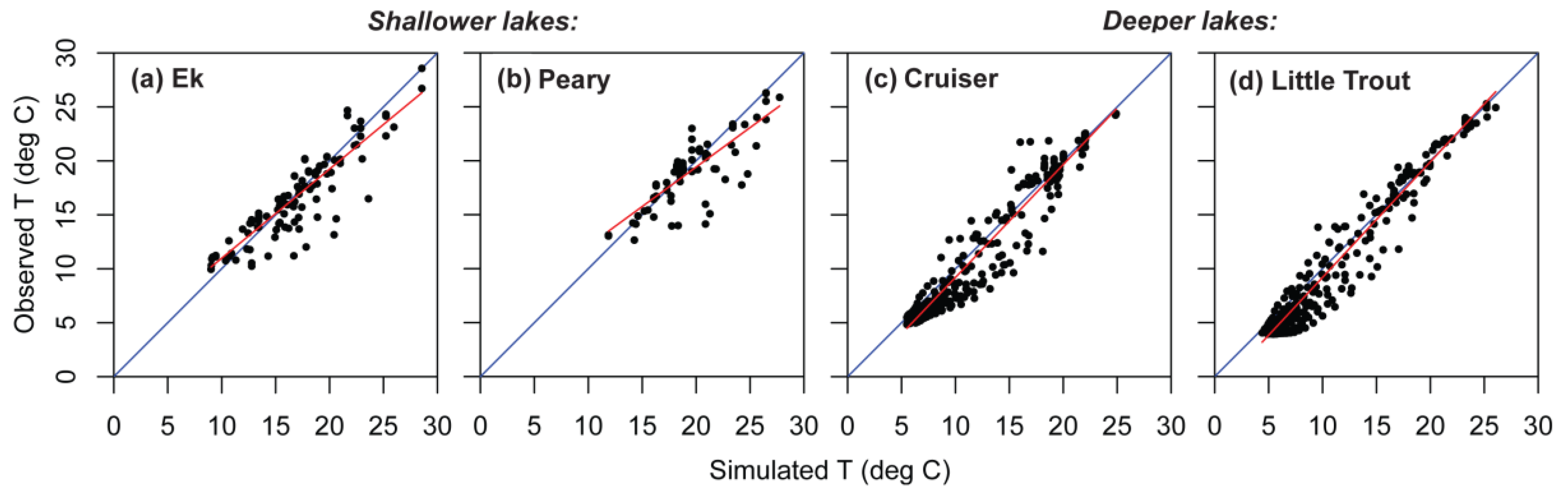
Figure 6.
Observed versus simulated temperatures (T), showing regression line (red) through the cloud of observed values and the 1:1 line (blue) for four lakes in Voyageurs National Park. (a) Shallow Ek Lake; (b) shallow Peary Lake; (c) deep Cruiser Lake; (d) deep Little Trout Lake.
Figure 6.
Observed versus simulated temperatures (T), showing regression line (red) through the cloud of observed values and the 1:1 line (blue) for four lakes in Voyageurs National Park. (a) Shallow Ek Lake; (b) shallow Peary Lake; (c) deep Cruiser Lake; (d) deep Little Trout Lake.
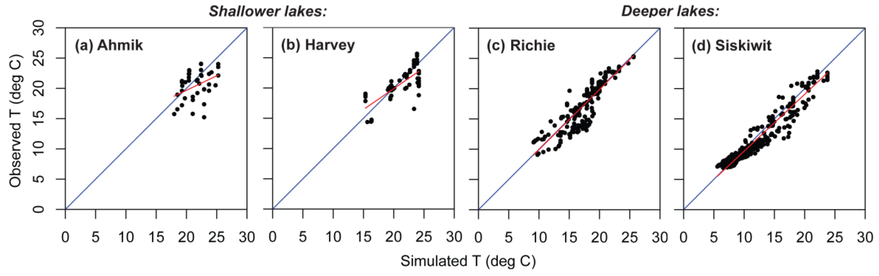
Figure 7.
Observed versus simulated temperatures (T), showing regression line (red) through the cloud of observed values and the 1:1 line (blue) for four lakes in Isle Royale National Park. (a) Shallow Ahmik Lake; (b) shallow Harvey Lake; (c) deep Richie Lake; (d) deep Siskiwit Lake.
Figure 7.
Observed versus simulated temperatures (T), showing regression line (red) through the cloud of observed values and the 1:1 line (blue) for four lakes in Isle Royale National Park. (a) Shallow Ahmik Lake; (b) shallow Harvey Lake; (c) deep Richie Lake; (d) deep Siskiwit Lake.
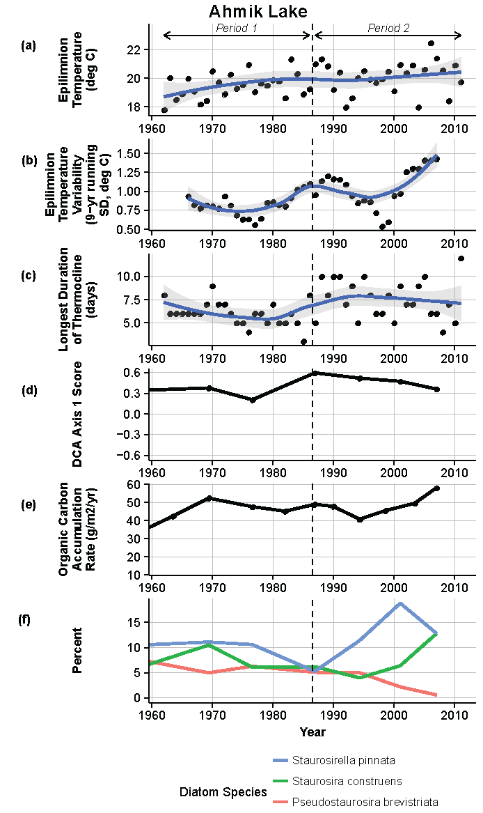
Figure 8.
Model results and paleolimnological data for Ahmik Lake, Isle Royale National Park, 1960–2011. (a) Epilimnion temperature (°C); (b) nine-year running average of epilimnion temperature (SD, °C); (c) longest duration of thermocline (days); (d) diatom species turnover, detrended correspondence analysis (DCA) axis 1 score; (e) organic carbon accumulation rate (g/m2/year); (f) percent abundance of common diatom species, Staurosirella pinnata, Staurosira construens, Pseudostaurosira brevistriata.
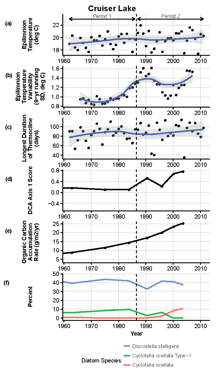
Figure 9.
Model results and paleolimnological data for Cruiser Lake, Voyageurs National Park, 1960–2011. (a) Epilimnion temperature (°C); (b) nine-year running average of epilimnion temperature (SD, °C); (c) longest duration of thermocline (days); (d) diatom species turnover, DCA axis 1 score; (e) organic carbon accumulation rate (g/m2/year); (f) percent abundance of common diatom species, Discostella stelligera, Cyclotella ocellata—Type 1, Cyclotella ocellata.
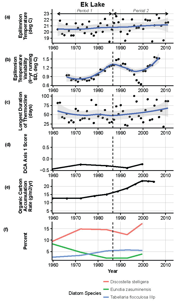
Figure 10.
Model results and paleolimnological data for Ek Lake, Voyageurs National Park, 1960–2011. (a) Epilimnion temperature (°C); (b) nine-year running average of epilimnion temperature (SD, °C); (c) longest duration of thermocline (days); (d) diatom species turnover, DCA axis 1 score; (e) organic carbon accumulation rate (g/m2/year); (f) percent abundance of common diatom species, Discostella stelligera, Eunotia zasuminensis, Tabellaria flocculosa IIIp.
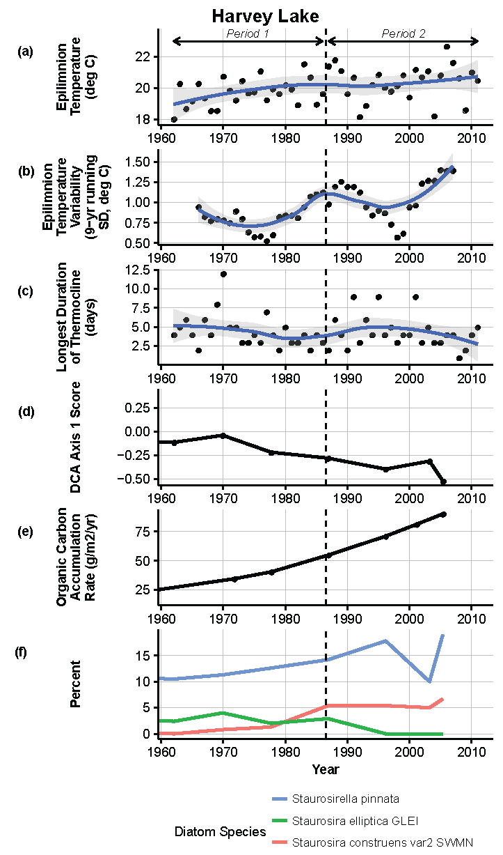
Figure 11.
Model results and paleolimnological data for Harvey Lake, Isle Royale National Park, 1960–2011. (a) Epilimnion temperature (°C); (b) nine-year running average of epilimnion temperature (SD, °C); (c) longest duration of thermocline (days); (d) diatom species turnover, DCA axis 1 score; (e) organic carbon accumulation rate (g/m2/year); (f) percent abundance of common diatom species, Staurosirella pinnata, Staurosira elliptica GLEI, Staurosira construens v. 2SWMN.
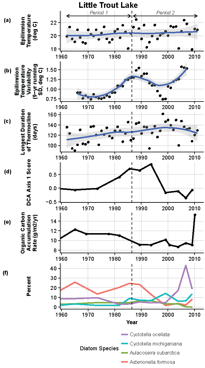
Figure 12.
Model results and paleolimnological data for Little Trout Lake, Voyageurs National Park, 1960–2011. (a) Epilimnion temperature (°C); (b) nine-year running average of epilimnion temperature (SD, °C); (c) longest duration of thermocline (days); (d) diatom species turnover, DCA axis 1 score; (e) organic carbon accumulation rate (g/m2/year); (f) percent abundance of common diatom species, Cyclotella ocellata, C. michiganiana, Aulacoseira subarctica, Asterionella formosa.
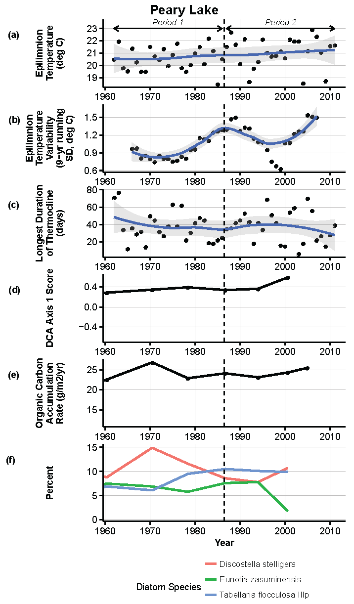
Figure 13.
Model results and paleolimnological data for Peary Lake, Voyageurs National Park, 1960–2011. (a) Epilimnion temperature (°C); (b) nine-year running average of epilimnion temperature (SD, °C); (c) longest duration of thermocline (days); (d) diatom species turnover, DCA axis 1 score; (e) organic carbon accumulation rate (g/m2/year); (f) percent abundance of common diatom species, Discostella stelligera, Eunotia zasuminensis, Tabellaria flocculosa IIIp.
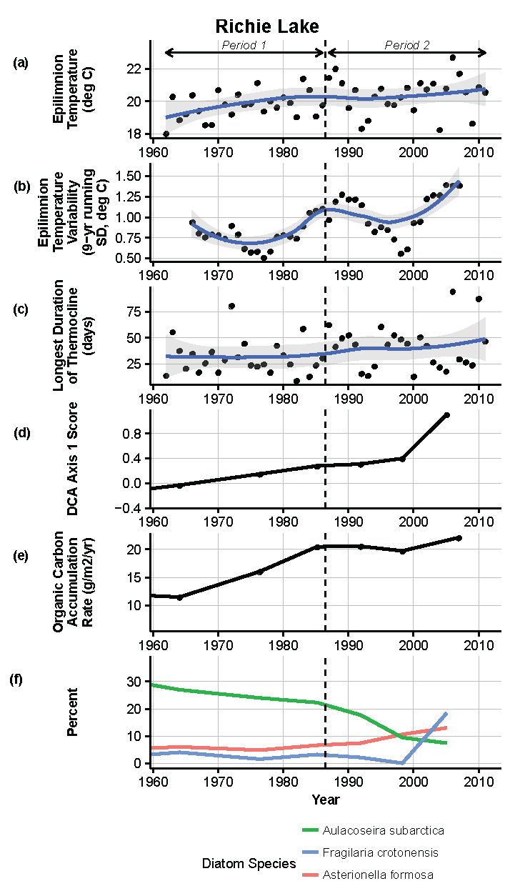
Figure 14.
Model results and paleolimnological data for Richie Lake, Isle Royale National Park, 1960–2011. (a) Epilimnion temperature (°C); (b) nine-year running average of epilimnion temperature (SD, °C); (c) longest duration of thermocline (days); (d) diatom species turnover, DCA axis 1 score; (e) organic carbon accumulation rate (g/m2/year); (f) percent abundance of common diatom species, Aulacoseira subarctica, Fragilaria crotonensis, Asterionella formosa.
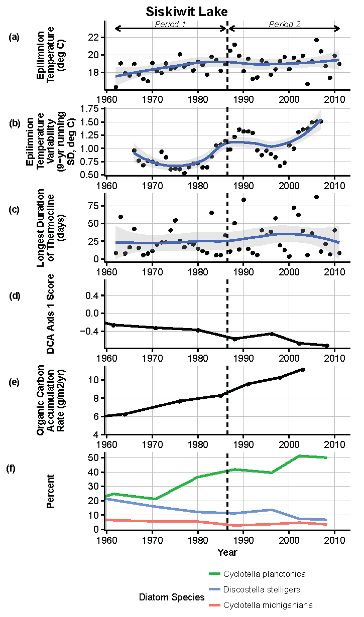
Figure 15.
Model results and paleolimnological data for Siskiwit Lake, Isle Royale National Park, 1960–2011. (a) Epilimnion temperature (°C); (b) nine-year running average of epilimnion temperature (SD, °C); (c) longest duration of thermocline (days); (d) diatom species turnover, DCA axis 1 score; (e) organic carbon accumulation rate (g/m2/year); (f) percent abundance of common diatom species, Cyclotella planctonica, Discostella stelligera, C. michiganiana.
Table 1.
Study lake locations and assembled background data 1.
Table 1.
Study lake locations and assembled background data 1.
| Park Unit | Lat | Lon | Alt | Area | Aws | Inlets | Outlets | Zmax | Zseci | TP | Chl a | DOC |
|---|
| Lake | degrees | degrees | (m) | (ha) | (ha) | | | (m) | (m) | (μg/L) | (μg/L) | (mg/L) |
| VOYA | | | | | | | | | | | | |
| Cruiser | 48.498 | −92.805 | 380 | 47.3 | 118 | 1 | 1 | 28.8 | 7.72 | 3.8 | 0.9 | 4.2 |
| Ek | 48.470 | −92.836 | 346 | 36.3 | 250 | 3 | 1 | 6.2 | 2.01 | 18.5 | 6.8 | 13.2 |
| Little Trout | 48.397 | −92.523 | 349 | 104.0 | 236 | 0 | 1 | 30.0 | 6.40 | 4.4 | 1.1 | 5.0 |
| Peary | 48.525 | −92.771 | 343 | 44.8 | 976 | 3 | 1 | 5.2 | 2.51 | 17.5 | 5.6 | 10.1 |
| ISRO | | | | | | | | | | | | |
| Ahmik | 48.150 | −88.539 | 190 | 8.5 | 36 | 1 | 1 | 2.9 | 2.17 | 20.1 | 2.5 | 17.8 |
| Harvey | 48.050 | −88.800 | 233 | 53.4 | 341 | 6 | 1 | 5.0 | 3.39 | 14.8 | 2.1 | 10.1 |
| Richie | 48.043 | −88.693 | 190 | 204.7 | 1956 | 4 | 1 | 11.1 | 1.80 | 26.1 | 6.4 | 9.9 |
| Siskiwit | 48.000 | −88.800 | 197 | 1687.4 | 7239 | 10 | 1 | 47.3 | 7.36 | 4.2 | 0.9 | 5.2 |
Table 2.
Definitions of general lake categories based on maximum depth, area, and Secchi-disk depth 1.
Table 2.
Definitions of general lake categories based on maximum depth, area, and Secchi-disk depth 1.
| Parameter | Category | Minimum | Maximum | Typical |
|---|
| Maximum Depth, Zmax (m) | Shallow | 0 | 4 | 4 |
| Medium | 4 | 20 | 13 |
| Deep | 20 | 45 | 24 |
| Lake Area (km2) | Small | 0 | 0.4 | 0.2 |
| Medium | 0.4 | 5 | 1.7 |
| Large | 5 | 40 | 10 |
| Secchi-Disk Depth, Zseci (m) | Eutrophic | 0 | 1.8 | 1.2 |
| Mesotrophic | 1.8 | 4.5 | 2.5 |
| Oligotrophic | 4.5 | 7 | 4.5 |
Table 3.
Study lake categories based on size, trophic status, and stratification potential 1.
Table 3.
Study lake categories based on size, trophic status, and stratification potential 1.
| By Area | By Depth | Trophic Status | Stratification |
|---|
| Park Unit | | | Secchi | TP | Chl a | | |
| Lake | | | TSI | Class | TSI | Class | TSI | Class | GR | Class |
| VOYA | | | | | | | | | | |
| Cruiser | Medium | Deep | 31 | O | 23 | O | 30 | O | 0.9 | Strong |
| Ek | Small | Medium | 50 | M | 46 | M | 49 | M | 4.0 | Medium |
| Little Trout | Medium | Deep | 33 | O | 26 | O | 32 | O | 1.1 | Strong |
| Peary | Medium | Medium | 47 | M | 45 | M | 47 | M | 5.0 | Medium |
| ISRO | | | | | | | | | | |
| Ahmik | Small | Shallow | 49 | M | 47 | M | 39 | M | 6.2 | Weak |
| Harvey | Medium | Medium | 42 | M | 43 | M | 38 | O | 5.3 | Weak |
| Richie | Medium | Medium | 52 | E | 51 | M | 49 | M | 3.4 | Medium |
| Siskiwit | Large | Deep | 31 | O | 25 | O | 29 | O | 1.4 | Strong |
Table 4.
MINLAKE-specific parameters for study lakes 1.
Table 4.
MINLAKE-specific parameters for study lakes 1.
| Light Attenuation Parameters | Wind | SOD | BOD | Metalimnion | SOD | Hypolimnion | Lower |
|---|
| Total | Algal | Water | Sheltering | | | Diffusion | Multiplier | Diffusion | Chl a |
|---|
| From Zseci | From Chl a | By Diff | Coeff | | | Coefficient | | Coefficient | Multiplier |
|---|
| Park Unit | | | XK1 | Wstr | Sb20 | BOD | EMCOE(1) | EMCOE(2) | EMCOE(4) | EMCOE(5) |
| Lake | (per m) | (per m) | (per m) | | | (mg/L) | | | | |
| VOYA | | | | | | | | | | |
| Cruiser | 0.24 | 0.02 | 0.22 | 0.17 | 0.2 | 0.50 | 0.5 | 5.0 | 1.0 | 1.5 |
| Ek | 0.91 | 0.14 | 0.78 | 0.13 | 0.8 | 0.75 | 1.0 | 2.3 | 1.0 | 1.0 |
| Little Trout | 0.29 | 0.02 | 0.27 | 0.33 | 0.2 | 0.50 | 0.5 | 5.0 | 1.0 | 1.5 |
| Peary | 0.73 | 0.11 | 0.62 | 0.16 | 0.8 | 0.75 | 1.0 | 2.3 | 1.0 | 1.0 |
| ISRO | | | | | | | | | | |
| Ahmik | 0.85 | 0.05 | 0.80 | 0.04 | 1.0 | 0.75 | 1.0 | 1.9 | 1.0 | 1.0 |
| Harvey | 0.54 | 0.04 | 0.50 | 0.18 | 0.4 | 0.50 | 1.0 | 3.0 | 1.0 | 1.5 |
| Richie | 1.02 | 0.13 | 0.89 | 0.54 | 0.8 | 0.75 | 1.0 | 2.3 | 1.0 | 1.0 |
| Siskiwit | 0.25 | 0.02 | 0.23 | 1.00 | 0.2 | 0.50 | 0.5 | 5.0 | 1.0 | 1.5 |
Table 5.
Significance of change over time from the first half (1962–1986) to the second half (1987–2011) of the data set for selected climate variables 1.
Table 5.
Significance of change over time from the first half (1962–1986) to the second half (1987–2011) of the data set for selected climate variables 1.
| Temperature | Wind Speed | Solar Radiation | Rain | Snow |
|---|
| Climate Station | (°C) | (m/s) | (Langley) | (mm) | (mm) |
| Season | Mean | Mean | Mean | Sum | Sum |
| International Falls (for VOYA) | | | | | |
| Annual | <0.001 | <0.001 | 0.004 | 1.000 | 0.030 |
| Spring | 0.170 | <0.001 | <0.001 | 0.907 | 0.461 |
| Summer | 0.345 | <0.001 | 0.832 | 0.930 | NA |
| Fall | 0.077 | <0.001 | 0.043 | 0.686 | 0.174 |
| Winter | 0.001 | 0.001 | <0.001 | 0.833 | 0.034 |
| Duluth (for ISRO) | | | | | |
| Annual | <0.001 | <0.001 | 0.001 | 0.467 | 0.538 |
| Spring | 0.078 | 0.005 | <0.001 | 0.969 | 0.554 |
| Summer | 0.020 | 0.001 | 0.298 | 0.934 | NA |
| Fall | 0.108 | 0.030 | 0.104 | 0.554 | 0.015 |
| Winter | 0.002 | 0.010 | <0.001 | 0.715 | 0.923 |
Table 6.
Goodness-of-fit statistics relative to lake depths and range of observed temperatures 1.
Table 6.
Goodness-of-fit statistics relative to lake depths and range of observed temperatures 1.
| Statistics | Observations |
|---|
| Park Unit | NSE | R2 | RMSE | Mean Error | Zmax | N | Min | Max | Range |
| Lake | | | (°C) | (°C) | (m) | | (°C) | (°C) | (°C) |
| VOYA | | | | | | | | | |
| Peary | 0.58 | 0.69 | 2.1 | 0.4 | 5.2 | 85 | 12.7 | 26.3 | 13.7 |
| Ek | 0.74 | 0.78 | 2.0 | 0.2 | 6.2 | 112 | 10.0 | 28.6 | 18.6 |
| Cruiser | 0.92 | 0.94 | 1.7 | 0.7 | 28.8 | 363 | 4.8 | 24.4 | 19.5 |
| Little Trout | 0.94 | 0.96 | 1.6 | 0.8 | 30.0 | 384 | 3.9 | 25.3 | 21.4 |
| ISRO | | | | | | | | | |
| Ahmik | −0.25 | 0.15 | 2.7 | 1.1 | 2.9 | 41 | 15.2 | 24.1 | 8.8 |
| Harvey | 0.42 | 0.56 | 2.1 | 0.5 | 5.1 | 57 | 14.4 | 25.7 | 11.3 |
| Richie | 0.76 | 0.76 | 1.8 | 0.1 | 11.1 | 213 | 9.1 | 25.3 | 16.3 |
| Siskiwit | 0.92 | 0.94 | 1.3 | 0.5 | 45.3 | 357 | 6.9 | 22.8 | 15.9 |
Table 7.
Significance of change over time from the first half (1962–1986) to the second half (1987–2011) of MINLAKE runs for selected lake-thermal variables 1.
Table 7.
Significance of change over time from the first half (1962–1986) to the second half (1987–2011) of MINLAKE runs for selected lake-thermal variables 1.
| Lake | Peary | Ek | Cruiser | Little Trout | Ahmik | Harvey | Richie | Siskiwit |
|---|
| Park Unit | VOYA | VOYA | VOYA | VOYA | ISRO | ISRO | ISRO | ISRO |
| Zmax (maximum depth, m) | 5.2 | 6.2 | 28.8 | 30.0 | 2.9 | 5.1 | 11.1 | 47.3 |
| Area (ha) | 44.8 | 28.6 | 41.1 | 90.9 | 8.5 | 53.4 | 204.7 | 1687.4 |
| Geometric Ratio | 5.0 | 4.0 | 0.9 | 1.1 | 6.2 | 5.3 | 3.4 | 1.4 |
| Zseci (Secchi depth, m) | 2.5 | 2.0 | 7.7 | 6.4 | 2.2 | 3.4 | 1.8 | 7.4 |
| TP (total phosphorus, μg/L) | 17 | 18 | 4 | 4 | 20 | 15 | 26 | 4 |
| DOC (dissolved organic carbon, mg/L) | 10 | 13 | 4 | 5 | 18 | 10 | 10 | 5 |
| Aws (watershed area, ha) | 976 | 250 | 118 | 236 | 36 | 341 | 1956 | 7239 |
| Temperatures—summer (JJA) mean | | | | | | | | |
| Shallow (1 m) | 0.03 | 0.032 | 0.095 | 0.084 | 0.013 | 0.011 | 0.013 | 0.027 |
| Deep (0.9*Zmax) | 0.335 | 0.658 | 0.969 | 0.032 | 0.039 | 0.016 | 0.500 | 0.773 |
| Temperature Variability—SD of summer means | | | | | | | | |
| rolling SD of nine-year window of above means | | | | | | | | |
| Shallow (1 m) | 0.004 | <0.001 | <0.001 | <0.001 | <0.001 | <0.001 | <0.001 | <0.001 |
| Deep (0.9*Zmax) | <0.001 | <0.001 | 0.636 | 0.862 | 0.001 | 0.002 | 0.017 | <0.001 |
| Temperature gradients: >2 °C per m | | | | | | | | |
| First day of year with gradient | 0.854 | 0.698 | 0.109 | 0.763 | 0.793 | 0.398 | 0.248 | 0.052 |
| Last day of year with gradient | 0.081 | 0.114 | 0.037 | 0.669 | 0.393 | 0.443 | 0.528 | 0.052 |
| Total days with gradient | 0.892 | 0.225 | 0.264 | 0.061 | 0.793 | 0.192 | 0.024 | 0.084 |
| Longest duration with gradient | 0.861 | 0.299 | 0.204 | 0.009 | 0.009 | 0.851 | 0.058 | 0.449 |
| Longest duration with gradient, per m hypolimnion | 0.715 | 0.464 | 0.271 | 0.019 | 0.011 | 1.000 | 0.182 | 0.525 |
| Summertime (JJA) depth of gradient (mean) | 0.503 | 0.298 | 0.112 | 0.097 | 0.809 | 0.834 | <0.001 | 0.001 |
| Ice and Water | | | | | | | | |
| First day of open water | 0.793 | 0.808 | 0.869 | 1.000 | 0.272 | 0.232 | 0.248 | 0.372 |
| First day of continuous ice | 0.808 | 0.484 | 0.256 | 0.712 | 0.727 | 0.580 | 0.771 | 0.876 |
| Duration of continuous ice | 0.617 | 0.881 | 0.912 | 0.465 | 0.406 | 0.307 | 0.562 | 0.548 |
| Duration of open-water season | 0.892 | 0.771 | 0.900 | 0.655 | 0.299 | 0.190 | 0.210 | 0.277 |

 ,
, 


