

Using Automated Machine Learning for Spatial Prediction—The Heshan Soil Subgroups Case Study

1
Key Laboratory of Earthquake Prediction, Institute of Earthquake Forecasting, China Earthquake Administration, Beijing 100036, China
2
State Key Laboratory of Resources and Environmental Information System, Institute of Geographic Sciences and Natural Resources Research, Chinese Academy of Sciences, Beijing 100101, China
3
University of Chinese Academy of Sciences, Beijing 100049, China
4
School of Geography and Tourism, Shaanxi Normal University, Xi’an 710119, China
5
Jiangsu Center for Collaborative Innovation in Geographical Information Resource Development and Application, School of Geography, Nanjing Normal University, Nanjing 210097, China
6
Department of Geography, University of Wisconsin-Madison, Madison, WI 53706, USA
*
Author to whom correspondence should be addressed.
Land 2024, 13(4), 551; https://doi.org/10.3390/land13040551
Submission received: 6 March 2024
/
Revised: 17 April 2024
/
Accepted: 18 April 2024
/
Published: 20 April 2024
(This article belongs to the Special Issue Digital Soil Mapping for Agri-Environmental Management and Sustainability)
Abstract
:Recently, numerous spatial prediction methods with diverse characteristics have been developed. Selecting an appropriate spatial prediction method, along with its data preprocessing and parameter settings, presents a challenging task for many users, especially for non-experts. This paper addresses this challenge by exploring the potential of automated machine learning method proposed in artificial intelligent domain to automatically determine the most suitable method among various machine learning methods. As a case study, the automated machine learning method was applied to predict the spatial distribution of soil subgroups in Heshan farm. A total of 110 soil samples and 10 terrain variables were utilized in the designed experiments. To evaluate the performance, the proposed method was compared to each machine learning method with default parameters values or parameters determined by expert knowledge. The results showed that the proposed method typically achieved higher accuracy scores than the two alternative methods. This suggests that automated machine learning performs effectively in scenarios where numerous machine learning methods are available and offers practical utility in reducing the dependence on users’ expertise in spatial prediction. However, a more robust automated framework should be developed to encompass a broader range of spatial prediction methods, such as spatial statistic methods, rather than only focusing on machine learning methods.
1. Introduction
Spatial prediction (SP) is one of the major ways to quickly acquire the spatial distribution of target geographic variables, such as the distribution of soil subgroups or landslide susceptibility [1,2]. SP hinges upon capturing the spatial relationships between the target geographic variable and the environment using sample data, and then using the spatial relationship to predict the values of the target geographic variable at the unvisited positions [3,4,5,6]. Among the many steps involved in this process, determining an appropriate SP method to maximize the prediction performance from many available methods is a key and critical step that might significantly impact accuracy of the result.
Three approaches exist for determining appropriate SP methods. The first approach relies on the users’ own domain expert knowledge. In this approach, the users manually determine the proper SP methods based on their domain knowledge, such as statistical knowledge or experience. However, as the range of SP methods, including spatial statistical and machine learning (ML) methods, expands, most users usually lack the expert knowledge necessary to select appropriate SP methods. This could lead the users to use familiar or popular methods rather than the appropriate method [2].
The second approach involves developing guidelines or rules to assist in determining the appropriate SP method. In this approach, previous studies or experiences of determining SP methods are reviewed to find the factors that affect the selection of SP methods, and then a generic framework or rules are provided to assist users in selecting the appropriate SP method [7,8]. For instance, Gibert et al. proposed a two-step framework for determining appropriate SP methods: The first uses a conceptual map to categorize the SP methods based on the specified problem, followed by employing SP methods’ templates to guide users to determine the most suitable SP methods from a particular group [9]. This approach provides a useful guide for the users of SP methods, especially for the non-expert users of SP. However, due to the complexity of application scenarios, summarizing all the specific rules or metadata for the SP methods, under which each method exhibits an optimal performance, is often challenging. Furthermore, a lack of consensus persists regarding model selection guidelines [10].
The third group is the data-driven approaches that leverage field samples. In this approach, two or more SP methods would be selected as a candidate set for predicting, and then the SP method with the best performance with the users’ data can be selected as the final SP method. For instance, Pourghasemi and Rahmati employed ten SP methods for landslide susceptibility mapping in Iran and analyzed their performance [11]. Daviran et al. proposed a hybrid genetic-based random forest (RF) which could determine the hyperparameters of RF; their results affirmed the superiority of the automated way over the conventional RF with a default value [12]. Williams et al. developed a multiple objective optimization algorithm for model selection and successfully selected the suitable model [13]. The data-driven method could determine an appropriate SP method directly according to its predictive performance on the users’ data, which reduces dependence on expert knowledge. However, the final effectiveness of each SP method is always related to the data preprocessing and appropriate parameter settings of the SP method [14]. Data preprocessing encompasses various techniques such as selecting covariates, rescaling the data, encoding categorical covariates, imputation of the missing values and so on. Taking the covariates selection as an example, it is difficult to select covariates due to the multiple methods, each with advantages and disadvantages [15]. The SP methods and the preprocessing methods usually have lots of parameters, and application users must tune every parameter though cross-validation or domain knowledge. Moreover, tuning all possible values of the parameters is impractical. Currently, these laborious and knowledge-intensive operations often necessitate manual handling by users, which exceeds the capabilities of many users. This challenge could become more pronounced as the number of available SP methods continues to grow.
Automating these laborious and knowledge-intensive tasks could enhance the feasibility of the data-driven approach, especially for novice users. Recently, in the machine learning domain, automated machine learning (AutoML) has emerged to address the challenge of determining an appropriate ML method from various competing alternatives [16,17]. Can AutoML be utilized to aid users in automatically determining the best SP method? In this study, we conducted a case study on the classification of soil subgroups in Heshan farm to explore the feasibility and effectiveness of employing AutoML for determining SP methods.
2. The AutoML Approach
AutoML refers to a set of approaches that could automatically construct a proper ML method by consolidating the corresponding raw data preprocessing methods into a workflow, set the values of the parameters of methods used in the workflow and finally provide the users with a determined workflow that has the best performance on the application users’ data [16,17,18,19,20]. All processes involved in the workflow are based on the application users’ data with a constrained computational budget.
In AutoML, method selection and parameter setting are viewed as optimization problems, and a detailed definition is provided in reference [16]. The goal is to find the highest performing workflow with the corresponding parameter values based on the application users’ data by using optimization methods. The commonly used optimization methods include grid search [19], random search [21], Bayesian optimization [20] and so on. Owing to extensive data preprocessing and the ML methods that could be grouped into different workflows, coupled with the multitude of parameters within those methods, random search or grid search usually takes a long time, and trying all potential values of the parameters for all of the workflows is typically impractical [19,20,21]. Bayesian optimization could track past evaluation results to build a probabilistic model that could represent the probability score with the change in the parameters’ values [20]. Therefore, Bayesian optimization could reduce the search space and find the appropriate workflow quickly.
When an initial workflow is not provided, optimization methods usually begin with random initialization. However, experts eschew a random initialization but use the experience learned from previous tasks [22]. Consequently, many studies began to leverage knowledge from prior datasets to initialize the search space to determine this workflow. The knowledge pertains to the data preprocessing and ML methods with the best running performance on prior datasets. The Meta-learning or case-based method represents an effective use of the knowledge of prior datasets [23,24]. These methods could calculate the similarity between a new dataset and the prior datasets, subsequently utilizing the workflows of similar prior datasets as the initial search space.
Most optimization methods typically select one workflow with the best performance, resulting in the loss of the methods that perform almost as well as the final selected method. Some AutoML approaches are capable of storing those workflows and can automatically construct an ensemble for the final prediction. A determined workflow includes an ML method and the corresponding data preprocessing methods with determined parameter values. The ML methods in each workflow could be the same kind of machine learning method with different data preprocessing or different parameter values. Numerous studies show that an ensemble usually outperforms the single best workflow [2,25]. When building the ensemble, an important issue is setting the weight of each workflow. Common ensemble strategies include stacking, gradient-free numerical optimization and ensemble selection [26,27,28,29].
3. Implementation of AutoML
Auto-sklearn, a Python package, automatically determines the workflow of ML and data preprocessing methods [17]. Auto-sklearn encompasses numerous state-of-the-art ML algorithms and a suite of data pre-processing and predictor selection methods [30]. In this case study we employed the Auto-sklearn package to evaluate the explore the feasibility and effectiveness of AutoML in predicting soil subgroups.
4. Experiment Design
The spatial distribution of soil subgroups is a very important geographic variable and is usually the basic information for hydrological modeling, resource management and other geographical/environmental studies [4,31]. Thus, in this paper, predicting the spatial distribution of soil subgroups is taken as an example to evaluate the feasibility of AutoML for SP.
4.1. The Heshan Study Area
The study area is Heshan farm, which is located in the Heilongjiang province of China, with an elevation which ranges from 276 to 363 m (Figure 1). The area has a gentle slope with an average slope of 2° and has been cultivated as crop areas for more than 40 years. The main crops are wheat and soybean. Besides the valley bottom with fluvial deposits, the whole area is covered by silt loam loess. Due to the small area (i.e., 60 km2) of the study area, the macro climate conditions over the study area do not vary substantially [32]. The soil subgroups were classified at the subgroup level in the Chinese soil taxonomy system [33]. There are six main subgroups in total: Pachic Stagni-Udic Isohumosols (PSUI), Mollic Bori-Udic Cambosols (MBUC), Typic Hapli-Udic Isohumosols (THUI), Typic Bori-Udic Cambosols (TBUC), Lithic Udi-Orthic Primosols (LUOP) and Fibric Histic-Typic Haplic Stagnic Gleyosols (FHTHSG) [32].
4.2. Dataset
The database used in this study consisted of 110 samples, which were collected through four sampling strategies, including integrative hierarchical stepwise sampling, systematic sampling, subjective sampling and transect sampling [32].
Due to the small study area and the generally homogeneous parent material, the key environmental factors that influence the soil formation are the geomorphological structures. Thus, only terrain covariates were used for mapping in this study area. The Digital Elevation Model (DEM) with 10 m resolution was generated from a 1:10,000 scale topographic map. The Simple Digital Terrain Analysis software (SimDTA, version 1.0.3) was used to derive the other ten terrain covariates from the 10 m DEM [34]. These terrain covariates included slope, profile curvature, planform curvature, topographic wetness index, surface curvature index, landscape position index, relative position index, stream power index, topographic position index, terrain ruggedness index (Table 1).
4.3. Experimental Environments
4.4. Evaluation Method
4.4.1. Evaluation Aspects
In this study we evaluated the performance of the AutoML from two perspectives: (1) determining the workflow for each ML method individually; (2) assessing the performance of AutoML for a set of potential ML methods.
In the first perspective, AutoML was employed to automatically ascertain the data preprocessing methods for a specified ML method, subsequently configuring parameter values within this workflow. To evaluate the effectiveness of this AutoML, two additional approaches were designed. In the first approach, each ML method with default parameter values and devoid of preprocessing was utilized to predict the spatial distribution of the soil subgroups. In the second approach, the parameter values of the ML method were manually determined according to expert knowledge. Owing to the established performance in the digital soil mapping domain and the documented significant parameters that influence its performance, random forest was selected for comparative analysis between the AutoML and the expert knowledge. Considering the reported impact on the final performance of random forest in most prior studies [36,37], only three key parameters of random forest were used. Thus, we tuned those three parameters manually according to the previously reported knowledge in the second approach. The parameters include the number of trees to build the forest (ntree), the minimum number of samples used for the split at terminal tree node (nmin) and the number of covariates considered when looking for the best split (mtry). The parameter ntree was set to 1000 which is a large size of trees to make sure to achieve a stable result [38]. Consistent with prior studies, the parameter nmin was set to 5 [37,38]. A total of 11 covariates were used in this study, thus, the parameter mtry was set from 1 to 11, and the increment was set to 1.
In the second perspective, the objective was to assess the performance of AutoML in scenarios where numerous potential ML methods exist. The highest performing workflow constructed by AutoML was evaluated (“single workflow” for short). In addition, the performance of the ensemble built from a number of workflows by AutoML was also evaluated (“ensemble” for short). Both the single workflow and ensemble were then compared to the performance of ML methods determined individually by AutoML.
4.4.2. Cross-Validation and Evaluation Index
To examine the effectiveness of the proposed method for the two perspectives, 3-fold cross-validation was used. For the cross-validation, all the soil samples were randomly divided into 3 partitions. Two partitions were used to train the proposed method, and the remaining partition was used to assess the performance of the proposed method. This process was repeated 3 times, and each partition was treated as an evaluation set [39]. The performance measured by 3-fold cross-validation is the average of the accuracy scores computed in the 3 times loop. Due to the principles of optimization methods and the random setting of the initial workflows, the final performance of AutoML could vary. Therefore, we repeated the cross-validation process 30 times to illustrate the range of different performances. The 3-fold cross-validation was also applied to ML methods as default and expert approaches and repeated 30 times.
As a common evaluation index in multilabel classification, the overall accuracy score was used as the evaluation index [32]. The value of accuracy score ranges from 0 (the entire samples are predicted wrong) to 1 (the entire samples are predicted correctly).
where n is the number of samples and and are the original value and the predicted soil type for the ith sample, respectively.
5. Results
5.1. The Performance of the Determined ML Methods Using Different Ways When a Specified ML Method Exists
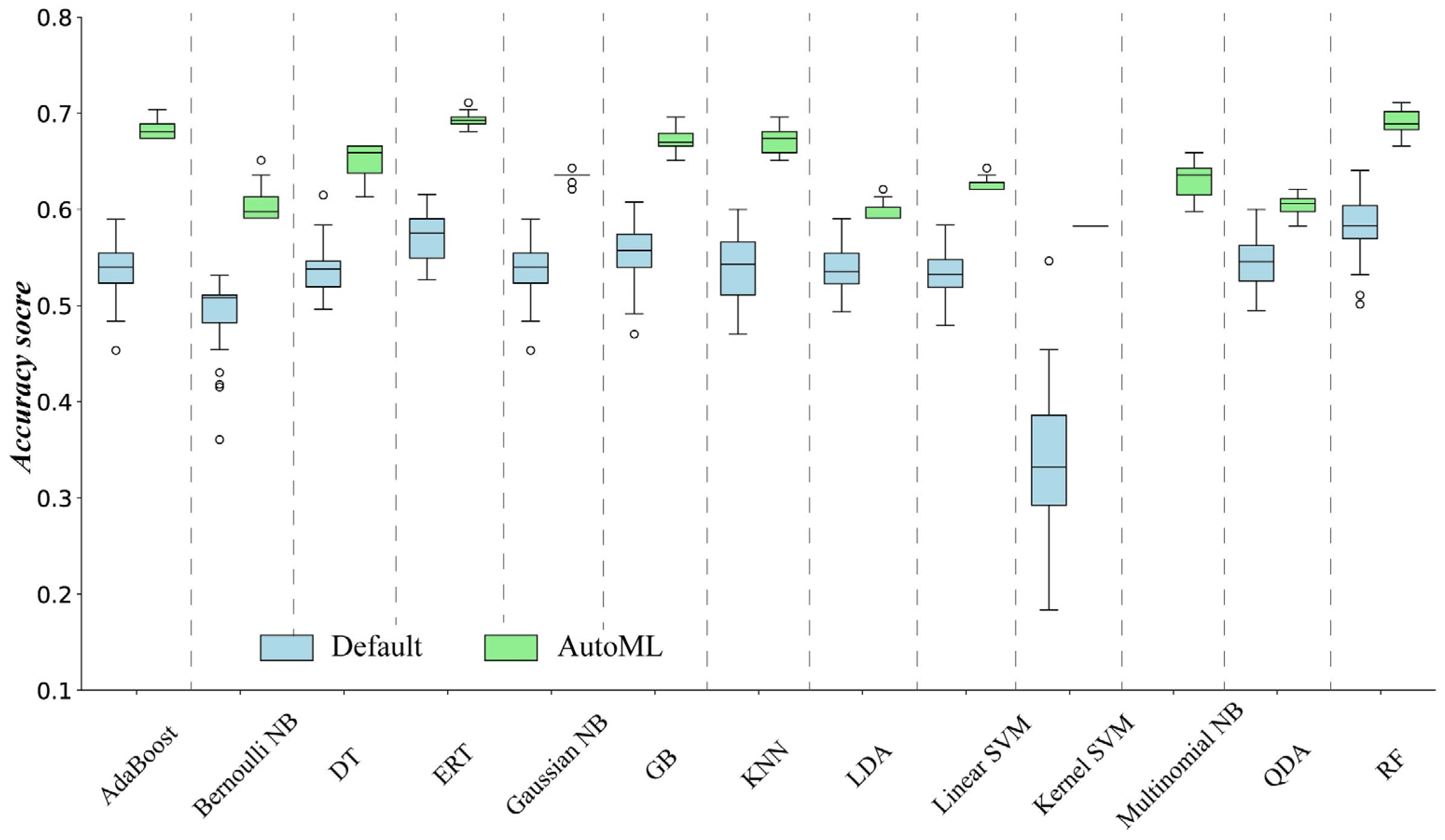
Figure 2 depicts a boxplot of the accuracy scores for the 13 ML methods which were determined through three different ways in the three-fold cross-validations with 30 repeats. Since Multinomial NB could not work without preprocessing the original data, it lacked accuracy scores with the default parameter values. The ML methods determined by AutoML consistently yielded higher accuracy scores than those with default parameter values (Figure 2). The performance of AutoML was 20% higher than the default for most of the ML methods. The accuracy scores of each ML method varied across the 30 repeats of three-fold cross-validation. The most important reason for this is that we randomly divided the samples into each of the three-fold cross-validations, which could have led to different training and evaluation samples across the 30 repeats.
The relative performances of the ML methods determined by AutoML and default had significant discrepancies (Figure 2). The performance of some ML methods was more similar when using AutoML. For example, the accuracy scores of AdaBoost were 6% lower than ERT with the default parameter values, while the accuracy scores of AdaBoost became almost as good as the ERT when the ML methods were determined using AutoML. Conversely, certain ML methods, such as the KNN and LDA, exhibited an increased performance gap under these conditions. Figure 3 shows the performance of RF determined using the three different ways, indicating that AutoM selected RF as a better performer compared to default and expert approaches.
5.2. The Performance of AutoML When Multiple Potential ML Methods Exist
Figure 4 illustrates the performance of AutoML which extended the number of potential ML methods from one to all thirteen. Under these conditions, the accuracy scores of the workflows determined by AutoML were very close to the highest performing workflows determined by AutoML for each ML method individually. In total, four ML methods were most selected by AutoML in the 30 repeated three-fold cross-validation, i.e., AdaBoost, DT, ERT, RF (Figure 5). Among those ML methods, the most selected ML methods (i.e., RF, ERT, AdaBoost) are the three highest performing methods when each ML method was determined by AutoML individually. However, other ML methods (e.g., DT) were also potentially selected by AutoML. This contributed to the lower accuracy scores compared to RF, ERT, AdaBoost which were determined by AutoML individually.
Compared to using a single workflow to predict the spatial distribution of soil subgroups, the ensemble had a slightly higher score (Figure 4). Each ensemble is usually constructed by a number of determined workflows (each workflow includes a ML method), ranged from 11 to 29 (Table 3). And the number of types of ML methods ranged from one to seven. The most selected ML methods were RF, AdaBoost, ERT which account 93.3% of all selected ML methods in the ensembles (Figure 6).
5.3. The Spatial Distribution of Soil Subgroups Predicted by AutoML
Figure 7 illustrates four maps of soil subgroups predicted by AutoML as examples. Notable differences can be seen between the maps predicted by the single workflow or the ensemble, particularly the spatial distribution of PSUI, TBUC and THUI. AutoML, as a data-driven approach, was significantly influenced by the soil samples. Consequently, the determined workflow constructed by AutoML could be very different when soil samples change. For instance, in the case of the two maps predicted by the single workflow, RF as the ML method employed select rates for covariate selection (Figure 7a), whereas ERT employed a polynomial (Figure 7b).
6. Discussion
6.1. The Potential Reason for the High Performance of AutoML
AutoML usually had higher performance than the two alternative approaches (i.e., the ML method with default parameter values and the ML method with parameter values manually determined according to expert knowledge). Although the performance of the manual approach exhibits higher values than the RF with the default parameter values, it still yields lower values than the AutoML approach (Figure 3). Two potential reasons could explain these results: (1) the manual approach only tuned the three most important parameters according to the expert knowledge while AutoML used all available parameters; (2) AutoML selected the proper data preprocessing methods for RF according to the original data from the users, including data normalization methods and the covariates selection methods.
6.2. The Influence of the Ensemble on the Performance of AutoML
The ensemble of various workflows did not exhibit significantly greater improvement than a single workflow with the best performance (Figure 4). However, as reported, combining numerous workflows into an ensemble can usually reduce the single workflow’s error and improve the final prediction result [2,17,40]. The possible reasons may be the small sample size and the ensemble strategy. Data-driven approaches typically need a large number of samples, particularly for highly complicated ML methods [41]. Additionally, the ensemble strategy used in Auto-sklearn was designed with a training samples dataset which exceeded 670 samples [17].
6.3. The Advantages of AutoML
AutoML is a practical approach for SP users, especially for non-experts. AutoML could help the SP users from two aspect: (1) it can automatically choose the best data preprocessing methods and the parameter value for a specified ML method; (2) it can determine the best ML methods and the corresponding data preprocessing parameters and their values using the numerous available ML methods. Compared to the way based on the users’ own domain knowledge, AutoML could reduce the burden to learn multiple domain knowledge and be more objective because the ML method is determined based on the field sampling data. Compared to the current guidelines or rules, AutoML could integrate more of the newest ML methods quickly without awaiting the development of more accurate and definite guidelines or rules. In addition, AutoML could tune all the parameters of the predictive and preprocessing methods, while expert domain knowledge is usually only concerned with some key parameters.
6.4. The Current Limitations and Future Work of the AutoML
The data-driven AutoML approach typically provides a black-box workflow which is usually hard to interpret [2,4,41]. AutoML randomly selects ML methods from a method set, then finds the best performing workflow based on optimization algorithms. In this process, the initial ML methods and the parameter values can affect the results of optimization algorithms. This is also the reason why some suboptimal predictive methods were also selected in our study (e.g., the DT selected in the single workflow in Figure 5).
In our study, AutoML only integrated 13 ML methods and 17 data preprocessing methods. However, many other powerful SP methods also exist, such as semi-supervised method [42], cubist [43,44], fuzzy membership [41], Regression kriging [45], geographically weighted regression [46] and so on. To make the AutoML more powerful in SP, it is necessary to integrate more SP and data preprocessing methods into the AutoML framework.
7. Conclusions
Determining an appropriate SP method is a pivotal step in spatial prediction. As a case study of AutoML, this paper used Auto-sklearn to determine the most appropriate ML methods in predicting the spatial distribution of soil subgroups on Heshan farm. This study assessed the feasibility and effectiveness of AutoML using a three-fold cross-validation method. Additionally, two alternative approaches for determining ML were designed to be compared with AutoML: (1) an ML method with default parameter values and (2) an ML method with parameter values determined based on expert knowledge. The primary findings of those experiments are outlined below:
- (1)
- Each ML method determined by AutoML outperformed those with default parameter values or determined by expert knowledge.
- (2)
- In scenarios where numerous ML methods are available, AutoML could also identify the highest performing ML method and implement the proper data preprocessing methods.
- (3)
- The accuracy and spatial distribution of soil subgroups predicted by AutoML closely depend on the sample database.
These findings demonstrate the practical utility of AutoML for SP users, particularly for non-experts. However, AutoML’s further developments should extend beyond ML methods to include other SP methods, such as the spatial statistics methods.
Author Contributions
Conceptualization, P.L. and C.-Z.Q.; methodology, P.L.; software, P.L.; validation, P.L.; formal analysis, P.L., C.-Z.Q., A.-X.Z. and P.L.; writing—original draft preparation, P.L.; writing—review and editing, C.-Z.Q. and A.-X.Z.; visualization, P.L.; supervision, C.-Z.Q. and A.-X.Z.; funding acquisition, C.-Z.Q. and P.L. All authors have read and agreed to the published version of the manuscript.
Funding
This work was supported by Science and Technology Fundamental Resources Investigation Program of China (Project No. 2021FY10010405), National Key Research and Development Program of China (Project No. 2021YFB3900904), LREIS [KPI003], and Shaanxi Normal University.
Data Availability Statement
The data presented in this study are available on request from the corresponding author. The data are not publicly available due to privacy restrictions.
Conflicts of Interest
The authors declare no conflicts of interest.
References
- Ayalew, L.; Yamagishi, H. The application of GIS-based logistic regression for landslide susceptibility mapping in the Kakuda-Yahiko Mountains, Central Japan. Geomorphology 2005, 65, 15–31. [Google Scholar] [CrossRef]
- Reichenbach, P.; Rossi, M.; Malamud, B.D.; Mihir, M.; Guzzetti, F. A review of statistically-based landslide susceptibility models. Earth-Sci. Rev. 2018, 180, 60–91. [Google Scholar] [CrossRef]
- McBratney, A.B.; Mendonça Santos, M.L.; Minasny, B. On Digital Soil Mapping. Geoderma 2003, 117, 3–52. [Google Scholar] [CrossRef]
- Heung, B.; Ho, H.C.; Zhang, J.; Knudby, A.; Bulmer, C.E.; Schmidt, M.G. An Overview and Comparison of Machine-Learning Techniques for Classification Purposes in Digital Soil Mapping. Geoderma 2016, 265, 62–77. [Google Scholar] [CrossRef]
- Zhu, A.X.; Lu, G.; Liu, J.; Qin, C.Z.; Zhou, C.H. Spatial prediction based on Third Law of Geography. Ann. GIS 2018, 24, 225–240. [Google Scholar] [CrossRef]
- Huang, Y.Y.; Song, X.D.; Wang, Y.P.; Canadell, J.G.; Luo, Y.Q.; Ciais, P.; Chen, A.P.; Hong, S.B.; Wang, Y.G.; Tao, F.; et al. Size, distribution, and vulnerability of the global soil inorganic carbon. Science 2024, 384, 233–239. [Google Scholar] [CrossRef] [PubMed]
- Wang, X.; Gu, W.; Ziebelin, D.; Hamilton, H. An ontology-based framework for geospatial clustering. Int. J. Geogr. Inf. Sci. 2010, 24, 1601–1630. [Google Scholar] [CrossRef]
- Li, J.; Heap, A.D. Spatial interpolation methods applied in the environmental sciences: A review. Environ. Model. Softw. 2014, 53, 173–189. [Google Scholar] [CrossRef]
- Gibert, K.; Izquierdo, J.; Sànchez-Marrè, M.; Hamilton, S.H.; Rodríguez-Roda, I.; Holmes, G. Which method to use? An assessment of data mining methods in Environmental Data Science. Environ. Model. Softw. 2018, 110, 3–27. [Google Scholar] [CrossRef]
- Hooten, M.B.; Hobbs, N.T. A guide to Bayesian model selection for ecologists. Ecol. Monogr. 2015, 85, 3–28. [Google Scholar] [CrossRef]
- Pourghasemi, H.R.; Rahmati, O. Prediction of the landslide susceptibility: Which algorithm, which precision? Catena 2018, 162, 177–192. [Google Scholar] [CrossRef]
- Daviran, M.; Maghsoudi, A.; Ghezelbash, R.; Pradhan, B. A New Strategy for Spatial Predictive Mapping of Mineral Prospectivity: Automated Hyperparameter Tuning of Random Forest Approach. Comput. Geosci. 2021, 148, 104688. [Google Scholar] [CrossRef]
- Williams, P.J.; Kendall, W.L.; Hooten, M.B. Selecting Ecological Models Using Multi-Objective Optimization. Ecol. Modell. 2019, 404, 21–26. [Google Scholar] [CrossRef]
- Clarke, B.; Fokoue, E.; Zhang, H.H. Principles and Theory for Data Mining and Machine Learning; Springer: New York, NY, USA, 2009; pp. 569–678. [Google Scholar]
- Fourcade, Y.; Besnard, A.G.; Secondi, J. Paintings predict the distribution of species, or the challenge of selecting environmental predictors and evaluation statistics. Glob. Ecol. Biogeogr. 2018, 27, 245–256. [Google Scholar] [CrossRef]
- Thornton, C.; Hutter, F.; Hoos, H.H.; Leyton-Brown, K. Auto-WEKA: Combined Selection and Hyperparameter Optimization of Classification Algorithms. In Proceedings of the 19th ACM SIGKDD International Conference on Knowledge Discovery and Data Mining, Chicago, IL, USA, 11–14 August 2013; pp. 847–855. [Google Scholar]
- Feurer, M.; Klein, A.; Eggensperger, K.; Springenberg, J.; Blum, M.; Hutter, F. Efficient and Robust Automated Machine Learning. In Proceedings of the 28th International Conference on Neural Information Processing Systems, Cambridge, MA, USA, 7–12 December 2015; pp. 2755–2763. [Google Scholar]
- Samanta, B. Gear fault detection using artificial neural networks and support vector machines with genetic algorithms. Mech. Syst. Signal Process. 2004, 18, 625–644. [Google Scholar] [CrossRef]
- Bergstra, J.S.; Bardenet, R.; Bengio, Y.; Kégl, B. Algorithms for Hyper-Parameter Optimization. In Proceedings of the 24th International Conference on Neural Information Processing Systems, New York, NY, USA, 12–15 December 2011; pp. 2546–2554. [Google Scholar]
- Snoek, J.; Larochelle, H.; Adams, R.P. Practical Bayesian Optimization of Machine Learning Algorithms. In Proceedings of the 25th International Conference on Neural Information Processing Systems, New York, NY, USA, 3–6 December 2012; pp. 2951–2959. [Google Scholar]
- Solis, F.J.; Wets, R.J.B. Minimization by Random Search Techniques. Math. Oper. Res. 1981, 6, 19–30. [Google Scholar] [CrossRef]
- Zöller, M.A.; Huber, M.F. Benchmark and Survey of Automated Machine Learning Frameworks. J. Artif. Intell. Res. 2021, 70, 409–472. [Google Scholar] [CrossRef]
- Vilalta, R.; Drissi, Y. A Perspective View and Survey of Meta-Learning. Artif. Intell. Rev. 2002, 18, 77–95. [Google Scholar] [CrossRef]
- Liang, P.; Qin, C.Z.; Zhu, A.X.; Hou, Z.W.; Fan, N.Q.; Wang, Y.J. A case-based method of selecting covariates for digital soil mapping. J. Integr. Agric. 2020, 19, 2127–2136. [Google Scholar] [CrossRef]
- Guyon, I.; Saffari, A.; Dror, G.; Cawley, G. Model Selection: Beyond the Bayesian/Frequentist Divide. J. Mach. Learn. Res. 2010, 11, 61–87. [Google Scholar]
- Wolpert, D.H. Stacked generalization. Neural Netw. 1992, 5, 241–259. [Google Scholar] [CrossRef]
- Caruana, R.; Niculescu-Mizil, A.; Crew, G.; Ksikes, A. Ensemble Selection from Libraries of Models. In Proceedings of the Twenty-First International Conference on Machine Learning, New York, NY, USA, 4–8 July 2004; p. 18. [Google Scholar]
- Kotthoff, L.; Thornton, C.; Hoos, H.H.; Hutter, F.; Leyton-Brown, K. Auto-WEKA 2.0: Automatic model selection and hyperparameter optimization in WEKA. J. Mach. Learn. Res. 2017, 18, 1–5. [Google Scholar]
- Mendoza, H.; Klein, A.; Feurer, M.; Springenberg, J.T.; Urban, M.; Burkart, M.; Dippel, M.; Lindauer, M.; Hutter, F. Towards Automatically-Tuned Deep Neural Networks. In Automated Machine Learning: Methods, Systems, Challenges; Hutter, F., Kotthoff, L., Vanschoren, J., Eds.; Springer: Cham, Switzerland, 2019; pp. 135–149. [Google Scholar]
- Pedregosa, F.; Varoquaux, G.; Gramfort, A.; Michel, V.; Thirion, B.; Grisel, O.; Blondel, M.; Prettenhofer, P.; Weiss, R.; Dubourg, V.; et al. Scikit-learn: Machine Learning in Python. J. Mach. Learn. Res. 2011, 12, 2825–2830. [Google Scholar]
- Rossiter, D.G.; Zeng, R.; Zhang, G.L. Accounting for taxonomic distance in accuracy assessment of soil class predictions. Geoderma 2017, 292, 118–127. [Google Scholar] [CrossRef]
- Zeng, C.; Yang, L.; Zhu, A.X.; Rossiter, D.G.; Liu, J.; Liu, J.Z.; Qin, C.Z.; Wang, D. Mapping soil organic matter concentration at different scales using a mixed geographically weighted regression method. Geoderma 2016, 281, 69–82. [Google Scholar] [CrossRef]
- Chinese Soil Taxonomy Research Group. Keys to Chinese Soil Taxonomy, 3rd ed.; University of Science and Technology of China Press: Hefei, China, 2001. [Google Scholar]
- Qin, C.Z.; Zhu, A.X.; Shi, X.; Li, B.L.; Pei, T.; Zhou, C.H. Quantification of spatial gradation of slope positions. Geomorphology 2009, 110, 152–161. [Google Scholar] [CrossRef]
- Wadoux, A.M.J.C.; Minasny, B.; McBratney, A.B. Machine Learning for Digital Soil Mapping: Applications, Challenges and Suggested Solutions. Earth Sci. Rev. 2020, 210, 103359. [Google Scholar] [CrossRef]
- Jeong, G.; Oeverdieck, H.; Park, S.J.; Huwe, B.; Ließ, M. Spatial soil nutrients prediction using three supervised learning methods for assessment of land potentials in complex terrain. Catena 2017, 154, 73–84. [Google Scholar] [CrossRef]
- Bouslihim, Y.; John, K.; Miftah, A.; Azmi, R.; Aboutayeb, R.; Bouasria, A.; Razouk, R.; Hssaini, L. The Effect of Covariates on Soil Organic Matter and pH Variability: A Digital Soil Mapping Approach Using Random Forest Model. Ann. GIS 2024, 1–18. [Google Scholar] [CrossRef]
- Grimm, R.; Behrens, T.; Märker, M.; Elsenbeer, H. Soil organic carbon concentrations and stocks on Barro Colorado Island—Digital soil mapping using Random Forests analysis. Geoderma 2008, 146, 102–113. [Google Scholar] [CrossRef]
- Poggio, L.; de Sousa, L.M.; Batjes, N.H.; Heuvelink, G.B.M.; Kempen, B.; Ribeiro, E.; Rossiter, D. SoilGrids 2.0: Producing soil information for the globe with quantified spatial uncertainty. SOIL 2021, 7, 217–240. [Google Scholar] [CrossRef]
- Rossi, M.; Guzzetti, F.; Reichenbach, P.; Mondini, A.C.; Peruccacci, S. Optimal landslide susceptibility zonation based on multiple forecasts. Geomorphology 2010, 114, 129–142. [Google Scholar] [CrossRef]
- Zhu, A.X.; Wang, R.; Qiao, J.; Qin, C.Z.; Chen, Y.; Liu, J.; Du, F.; Lin, Y.; Zhu, T. An expert knowledge-based approach to landslide susceptibility mapping using GIS and fuzzy logic. Geomorphology 2014, 214, 128–138. [Google Scholar] [CrossRef]
- Liu, H.; Shi, T.; Chen, Y.; Wang, J.; Fei, T.; Wu, G. Improving Spectral Estimation of Soil Organic Carbon Content through Semi-Supervised Regression. Remote Sens. 2017, 9, 29. [Google Scholar] [CrossRef]
- Henderson, B.L.; Bui, E.N.; Moran, C.J.; Simon, D.A.P. Australia-wide predictions of soil properties using decision trees. Geoderma 2005, 124, 383–398. [Google Scholar] [CrossRef]
- Bonfatti, B.R.; Hartemink, A.E.; Giasson, E.; Tornquist, C.G.; Adhikari, K. Digital mapping of soil carbon in a viticultural region of Southern Brazil. Geoderma 2016, 261, 204–221. [Google Scholar] [CrossRef]
- Odeh, I.O.A.; McBratney, A.B.; Chittleborough, D.J. Further results on prediction of soil properties from terrain attributes: Heterotopic cokriging and regression-kriging. Geoderma 1995, 67, 215–226. [Google Scholar] [CrossRef]
- Sharma, A. Exploratory Spatial Analysis of Food Insecurity and Diabetes: An Application of Multiscale Geographically Weighted Regression. Ann. GIS 2023, 2, 485–498. [Google Scholar] [CrossRef]
Figure 1.
The Heshan study area.

Figure 2.
Boxplot of accuracy scores for ML methods determined by different approaches.

Figure 3.
Boxplot of accuracy scores for RF which determined by default, expert and AutoML, respectively.
Figure 3.
Boxplot of accuracy scores for RF which determined by default, expert and AutoML, respectively.

Figure 4.
Boxplot of accuracy scores for the determined workflows by AutoML.

Figure 5.
The proportion of the ML methods selected by AutoML for the single workflows in 3-fold cross-validations with 30 repeats.
Figure 5.
The proportion of the ML methods selected by AutoML for the single workflows in 3-fold cross-validations with 30 repeats.

Figure 6.
The proportion of the ML methods selected by AutoML to construct the ensembles in 30 repetitive 3-fold cross-validations.
Figure 6.
The proportion of the ML methods selected by AutoML to construct the ensembles in 30 repetitive 3-fold cross-validations.

Figure 7.
The spatial distribution of soil subgroups generated by AutoML. (a,b) represent the maps with the best and worst evaluation accuracy scores by single workflow, respectively. (c,d) stand for the maps with the best and worst evaluation accuracy scores by the ensemble, respectively.
Figure 7.
The spatial distribution of soil subgroups generated by AutoML. (a,b) represent the maps with the best and worst evaluation accuracy scores by single workflow, respectively. (c,d) stand for the maps with the best and worst evaluation accuracy scores by the ensemble, respectively.


Table 1.
Covariates used in Heshan study area.
| Variables | Scale/ Resolution | Mean (Range) |
|---|---|---|
| Elevation | 10 m | 322 (276–363) |
| Slope | 10 m | 2 (0–17) |
| Profile curvature (ProCur) | 10 m | 0 (−0.01–0.01) |
| Planform curvature (PlanCur) | 10 m | 0 (−1.88–1.57) |
| Topographic wetness index (TWI) | 10 m | 9.38 (4.69–22) |
| Surface Curvature Index (CS) | 10 m | 0 (−0.023–0.016) |
| Landscape Position Index (LPos) | 10 m | 0 (−0.064–0.083) |
| Relative Position Index (RPI) | 10 m | 0.47 (0–1) |
| Stream Power Index (SPI) | 10 m | 32.4 (0–8281) |
| Topographic Position Index (TPI) | 10 m | 0 (−2.57–1.81) |
| Terrain Ruggedness Index (TRI) | 10 m | 0.31 (−0.001–2.75) |
Table 2.
The ML and data preprocessing methods used for selection in this study.
| Method Type | Methods |
|---|---|
| Data preprocessing methods | Balancing class weight, Extremely Randomized Trees, Fast Independent Component Analysis, Feature Agglomeration, Imputation of missing values, Kernel principal component analysis, Linear Support Vector Machines, No preprocessing, Normalization, Nystroem Method for Kernel Approximation, One hot encoding, Polynomial, Principal component analysis, Random Forest, Random Kitchen Sinks, Select percentile, Select rates |
| Classification methods | AdaBoost, Bernoulli Naive Bayes (Bernoulli NB), Decision tree (DT), Extremely Randomized Trees (ERT), Gaussian Naive Bayes (Gaussian NB), Gradient Boosting (GB), Kernel SVM, K-Nearest Neighbors (KNN), Linear Discriminant Analysis (LDA), Linear SVM, Multinomial Naive Bayes (Multi NB), Quadratic Discriminant Analysis (QDA), Random Forest (RF) |
Table 3.
Statistics of the number of workflows and the kind of ML methods used in each ensemble.
| Median | Min. | Max. | Std. | |
|---|---|---|---|---|
| Workflows | 20 | 11 | 29 | 5.58 |
| The kind of ML methods | 3 | 1 | 7 | 1.4 |
Disclaimer/Publisher’s Note: The statements, opinions and data contained in all publications are solely those of the individual author(s) and contributor(s) and not of MDPI and/or the editor(s). MDPI and/or the editor(s) disclaim responsibility for any injury to people or property resulting from any ideas, methods, instructions or products referred to in the content. |
© 2024 by the authors. Licensee MDPI, Basel, Switzerland. This article is an open access article distributed under the terms and conditions of the Creative Commons Attribution (CC BY) license (https://creativecommons.org/licenses/by/4.0/).
Share and Cite
MDPI and ACS Style
Liang, P.; Qin, C.-Z.; Zhu, A.-X. Using Automated Machine Learning for Spatial Prediction—The Heshan Soil Subgroups Case Study. Land 2024, 13, 551. https://doi.org/10.3390/land13040551
AMA Style
Liang P, Qin C-Z, Zhu A-X. Using Automated Machine Learning for Spatial Prediction—The Heshan Soil Subgroups Case Study. Land. 2024; 13(4):551. https://doi.org/10.3390/land13040551
Chicago/Turabian StyleLiang, Peng, Cheng-Zhi Qin, and A-Xing Zhu. 2024. "Using Automated Machine Learning for Spatial Prediction—The Heshan Soil Subgroups Case Study" Land 13, no. 4: 551. https://doi.org/10.3390/land13040551
Note that from the first issue of 2016, this journal uses article numbers instead of page numbers. See further details here.