Article

How to Realize Synergistic Emission Reduction in Future Urban Agglomerations: Spatial Planning Approaches to Reducing Carbon Emissions from Land Use: A Case Study of the Beijing–Tianjin–Hebei Region

1
School of Landscape Architecture, Beijing Forestry University, Beijing 100083, China
2
The Collaborative Innovation Center of the Beijing–Tianjin–Hebei, National Forestry and Grassland Administration, Beijing 100080, China
*
Author to whom correspondence should be addressed.
Land 2024, 13(4), 554; https://doi.org/10.3390/land13040554
Submission received: 25 March 2024 / Revised: 15 April 2024 / Accepted: 18 April 2024 / Published: 21 April 2024
(This article belongs to the Section Land Planning and Landscape Architecture)

Abstract

:
Land use changes in rapidly urbanizing regions around the world constitute a principal anthropogenic element fueling the surge in carbon emissions. Here, land use patterns within the Beijing–Tianjin–Hebei (BTH) urban agglomeration under low-carbon development (LCD) scenarios were simulated. Additionally, social network analysis was employed to formulate carbon balance planning guidelines for various administrative regions. (1) In the ecological protection scenario, carbon emissions from land use were 643.42 × 10⁴ tons lower compared to the natural development scenario. Counties with high ecological support coefficients accounted for 22%, making them better suited for predicting outcomes related to low-carbon-oriented land use. (2) The spatial connections of carbon emissions in BTH were closely related, forming the three main carbon emission spatial linkage areas. (3) A carbon balance zoning plan for the BTH in 2035 under the LCD scenario was formulated. Furthermore, key areas for the implementation of carbon peak and carbon neutrality projects were delineated, and targeted measures for carbon reduction and sink increase were proposed. This study provides a new perspective for implementing territorial spatial planning in Chinese urban agglomerations and can aid the government in formulating a reasonable low-carbon-oriented regional planning policy.

1. Introduction

Global warming is a growing concern and has become one of the major environmental challenges confronting the world presently. Carbon dioxide (CO2) is a greenhouse gas that is sourced mainly from man-made emissions, and its excessive emissions put significant pressure on the ecological environment [1,2]. Cities are densely populated and have become hot spots for CO2 emissions, with China’s urban areas accounting for 75% of the country’s overall carbon emissions [3]. Urban agglomeration is a key factor for promoting urban–rural integration and coordinated regional development [4]. In the process of achieving a low-carbon transformation of urban and rural areas, it is crucial to formulate sink increase and emission reduction strategies at the urban agglomeration level.
Carbon emissions are limited by land use change, which can affect global climate change and the carbon cycle by altering the surface carbon process and the intensity of human energy consumption [5]. Carbon emissions resulting from land use/cover changes (LUCCs) surpass 30% of global man-made carbon emissions [6,7]. Therefore, scientifically simulating LUCCs and exploring land use patterns under future low-carbon development (LCD) scenarios both aid in finding ways to reduce carbon emissions.
Land use carbon emissions can be calculated in several ways. Many scholars have characterized CO2 emissions by calculating the carbon emissions from energy consumption [8]. This method has some limitations, however. The calculation results of this method can only be expressed numerically, making it difficult to locate specific geographic spaces and to demonstrate the similarities and differences in the spatial distribution of carbon emissions. Some studies have used a combination of land use layout and carbon emission factors to compute carbon emissions [9]. This method can effectively express the spatial differences in carbon emissions and provide a planning basis for carbon reduction measures in different regions, filling the gap in calculating carbon emissions based on energy. The future land use layout in different scenarios can be used to guide the use of various methods, including the cellular automata (CA) model [10,11], CLUE-S model [12], FLUS model [13], and PLUS model [14]. Among these methods, the PLUS model provides benefits of high simulation accuracy and rapid data processing speed. By introducing land expansion analysis strategies and multitype random patch-seed generation mechanisms, it effectively simulates the intricate evolution process of multiple land types. At present, multiple studies have made notable contributions to carbon reduction in Chinese urban agglomerations from the perspective of emission reduction technologies. Although the development space for technology emission reduction is constrained, the importance of a top-down systematic planning methodology is gradually becoming prominent [15]. As a hot spot for greenhouse gas emissions, urban agglomerations exhibit the uneven distribution of CO2 because of their imbalanced socioeconomic factors [16]. Exploring collaborative approaches to emission reduction in urban agglomerations can better demonstrate the importance of the urban network structure in reducing CO2 emissions in the process of urbanization, thereby better guiding emission reduction planning. The economic development levels and natural environments of different cities and counties vary, and as a result, their carbon emissions also vary. These differences directly affect different regions’ ability to achieve carbon peak targets. Therefore, policy makers must develop different carbon reduction strategies based on specific circumstances and the inherent emission differences of each city and county [17]. The economic and population mobility relationships among counties are complex. The carbon emissions of each county within the urban cluster are greatly affected by surrounding counties, making it difficult to separate a county from the urban cluster and address its carbon issues separately. Therefore, when studying carbon emission reduction issues in urban agglomerations, considering the connections of carbon emissions between cities is essential. Social network analysis (SNA) serves as an effective methodology for examining the spatial structure of urban agglomerations and the spatial connections among cities. SNA can be employed to explore the spatial correlation characteristics of carbon emissions in urban agglomerations and the specificity of different cities and counties in carbon emission networks. Lately, numerous scholars have utilized SNA to examine spatial coupling, spatial correlation, and dynamic evolution of the spatiotemporal patterns of carbon emissions among regions in terms of the spatial scale [18,19].
Still, many gaps exist in current research on carbon emissions within urban agglomerations. Because of a lack of data, most studies can focus only on the carbon emissions of some large cities with recorded data, and the research locations are individual, not universal. In addition, due to limited interannual records of historical data, the data analysis results are applicable only to the policies and economic conditions at that time, making it difficult to align with recent carbon emission reduction governance policies. Moreover, most carbon emission simulations focus only on simulating future land use patterns or providing macro-policy recommendations to reduce emissions and enhance foreign exchange in the research area as a whole [20]. Few studies have simulated the land use patterns of LCD scenarios or formulated detailed and feasible planning guidelines for different administrative regions informed by the location and socioeconomic attributes of cities [21]. The classification types and methods of carbon balance zoning, as well as the planning guidelines for different regions to undertake the functions of increasing emissions and reducing emissions, remain unclear, and the theoretical basis needs to be improved.
Combining the PLUS model with the SNA method can compensate for this lack of data and can simulate the spatial carbon emission linkage in the context of formulating LCD policies in the future. Therefore, these methods can be used to more effectively formulate planning strategies and achieve the goal of increasing foreign exchange and reducing emissions.
The Beijing–Tianjin–Hebei (BTH) urban amalgamation stands as one of China’s four national-level urban agglomerations, and it has a high proportion of heavy industry and significant deterioration of ecological functions [22], which puts significant pressure on economic development, industrial upgrading, and integrated development. The significant energy consumption and exhaust emissions in the BTH urban agglomeration have caused serious air pollution [23]. Thus, coordinating the development of the BTH integration is of overriding significance to plan for carbon balance zoning and formulate a scientific linkage emission reduction scheme. Given this imperative, our study delved into the land use pattern under the future LCD scenario and the spatial association of carbon emissions. We also developed a low-carbon-oriented carbon balance zoning planning and management scheme.

2. Study area and Materials

2.1. Study Area

The BTH includes 13 cities (113°27–119°50 E, 36°05–42°40 N) (Figure 1). Its total area spans 21.5 million km2 and is situated in the northeastern coastal plain of China. As the BTH is one of four national urban agglomerations, its coordinated and integrated development can effectively improve the layout and form of urban agglomerations and contribute to the construction of an environmentally friendly society. In 2015, the state released the Outline for Coordinated Development of the Beijing–Tianjin–Hebei Region, which clarifies the significance of ecological environmental protection and the synergy between emission reduction and sink increase.

2.2. Data Sources

The data utilized in this study comprise land use data, soil type data, annual mean temperature data, annual mean precipitation data, DEM data, nighttime light data, GDP data, population data, railway data, highway data, national highway data, river water data, national nature reserve data, and carbon emission calculation data (Table 1).

3. Methodology

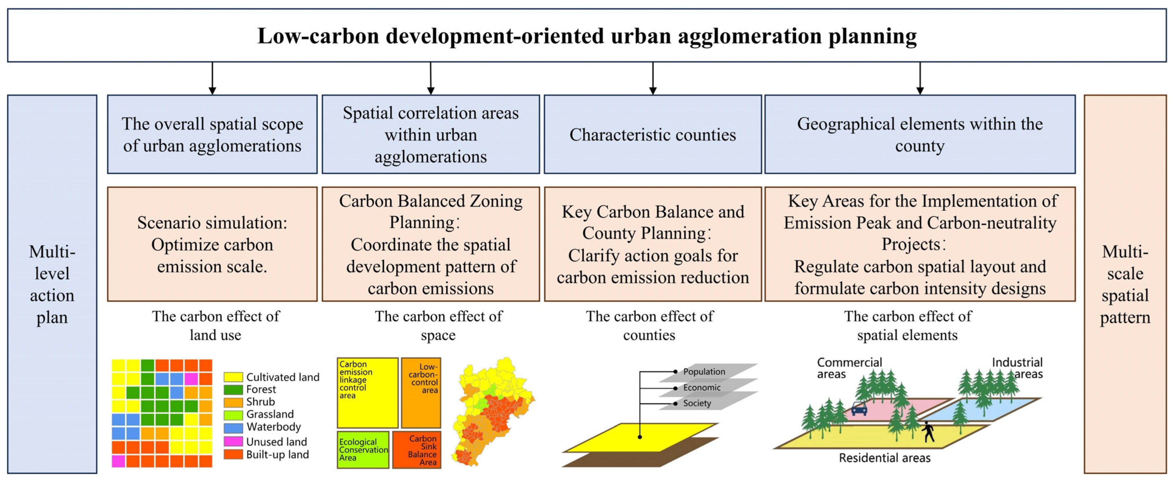
The proposed planning simulation framework in this study consists of three main components (Figure 2).
  • Land use pattern under the future LCD scenario: We used the PLUS model to import a dataset that includes land use data spanning three periods from 2010 to 2020, as well as climate, environment, and future driving factors to investigate the land use pattern under both the natural development (ND) scenario and ecological protection (EP) scenario in the BTH in 2035. We analyzed the carbon emission characteristics under the different scenarios and used the carbon emission and ecological support coefficient (ESC) as the criteria to screen the development scenarios that are more conducive to LCD scenarios.
  • Spatial connection analysis of carbon emissions under the LCD scenario: We introduced the carbon emission and socioeconomic data into the gravity model to formulate the carbon emission gravity matrix for the BTH region. We used SNA to assess the spatial network characteristics of carbon emissions in the BTH in 2035 under the LCD scenario.
  • Carbon balance zoning planning under the 2035 LCD scenario in the BTH: Drawing from the land use pattern under the LCD scenario and the spatial network characteristics of future carbon emissions, we analyzed the status and role of each region in increasing sinks and reducing emissions. On this basis, we formulated a future carbon balance zoning plan for the BTH to pinpoint critical areas for implementing the emission peak and carbon neutrality projects.

3.1. Multi-Scenario Land Use Pattern Projections

The PLUS model was derived from the FLUS model [26]. Drawing from the prediction of land use demand, the Markov module developed two modules: (1) land expansion strategy analysis (LEAS) and (2) the CA model of multitype random patch seeds (CARS). CARS can be used for refined land use simulation and prediction and can be coupled with a multi-objective optimization algorithm. The simulation outcomes can provide enhanced support for formulating planning policies to attain sustainable development goals.
To explore the land use patterns under various development scenarios, in the PLUS model, we established two development scenarios (ND and EP) to simulate the land use patterns in the BTH region for the year 2035. The ND scenario continued the development trend from 2010 to 2020 and maintained the transfer probability and neighborhood weight of the original land use types. Under the EP scenario, the primary goal orientation was the protection of the ecological environment. It aimed to curb the unordered expansion of urban areas, decrease the likelihood of converting forest land, shrub, grassland, and water bodies into built-up land by 20%, elevate the likelihood of converting cultivated land into forest land by 60%, and augment the likelihood of converting cultivated land into shrub and grassland by 50% when setting the neighborhood weight [27]. These two scenarios both took the national nature reserves as the limited expansion area.

3.2. Carbon Emissions Accounting

3.2.1. Carbon Emission Calculation Model

Carbon emissions from the BTH region were computed based on land use patterns under various scenarios derived from the PLUS simulation. Built-up land and cultivated land served as the primary carbon sources in the urban agglomeration, whereas forest land, grassland, water bodies, and unused land acted as the primary carbon sinks in the urban agglomeration [28,29,30,31,32,33]. Based on the China carbon emission inventory coefficient, and a coefficient from the relevant literature [29], we formulated the carbon emission coefficient of land use in the BTH region, as presented in Table 2. The formula for the land use carbon emission estimation model is as follows [9]:
C e = e i = n = 1 n A i × a i ,
where C e is carbon emissions, e i is carbon emissions from a specific land use type, A i indicates the area of the ith land use type, and a i is the carbon emission coefficient of the i th land use type.

3.2.2. Ecological Support Coefficient

We used the ecological support coefficient (ESC) to assess the carbon sink capacity under different development scenarios [34,35]. ESC can gauge the ecological capacity’s contribution to carbon balance in each region, and its calculation formula is as follows:
E S C = C A i C A / C i C ,
where C i and C represent the carbon emissions from each county-level unit and the entire region, respectively, and C A i and C A are the carbon sequestration values of each county-level unit and the entire region, respectively. If E S C > 1 , the contribution rate of carbon absorption exceeds the contribution rate of carbon emissions, and this indicates a robust ecological carrying capacity for the county. If E S C < 1 , the region’s ecological carrying capacity is considered weak. Taking ESC as one of the evaluation bases, we selected the low-carbon-oriented development scenario in the multi-scenario land use pattern prediction study described in Section 4.1.3 and Section 4.1.4, which encompassed a higher proportion of counties with lower carbon emissions and E S C   values > 1 , as the LCD scenario. Then, we analyzed the spatial connection of carbon emissions under the subsequent low-carbon scenario.

3.3. Spatial Correlation Analysis of Carbon Emissions Based on SNA

In this study, we employed the gravity model to measure the economic and social links between regions. GDP, POP size, and carbon emissions were also incorporated into the gravity model to adjust and measure the intensity of the carbon emissions linkage between the counties in the BTH [36]. The calculation formula is as follows:
R i j = k i j × G i P i C i 3 × G j P j C j 3 d i j 2 , k = C i C i + C j ,
where R is the gravitational value; d is the spherical geographical distance between counties; G , P , and C are GDP, POP, and total carbon emissions, respectively; k is the adjustment factor of the carbon emission ratio of a county in the two-way relationship; and i and j represent two different counties.
The GDP and POP data for 2035 were predicted using the gray (1, 1) model (GM). As the growth and change trends of the GDP and POP data are complex and uncertain, GM is suitable for predicting the GDP and POP data for 2035 [37,38]. We selected the GDP data and population data from 2014 to 2020 for prediction. We obtained the GDP data from a previous study [39] and the population data from the LandScan population dataset The LandScan population data produced by the U.S. Department of Energy at Oak Ridge National Laboratory (ORNL) represents ambient population count (averaged over 24 h) at approximately 1 km2 resolution.
The main characteristics of the spatial network were the network spatial pattern and the centrality of each county. The network spatial pattern was used primarily to visualize the overall structure of the network, indicating the ability to achieve coordinated development among regions. Centrality was employed to examine the individual roles of each county in collaborative emission reduction within the network. It reflects the significance of carbon emission exchange between counties for the coordinated development of the entire network. As a result, we clarified the key counties with different carbon emission reduction attributes. The centrality selection indicators are given in Table 3 [17].

3.4. Carbon Balance Planning for the BTH Urban Agglomeration in 2035 under the LCD Scenario

3.4.1. Carbon Balance Zoning Planning

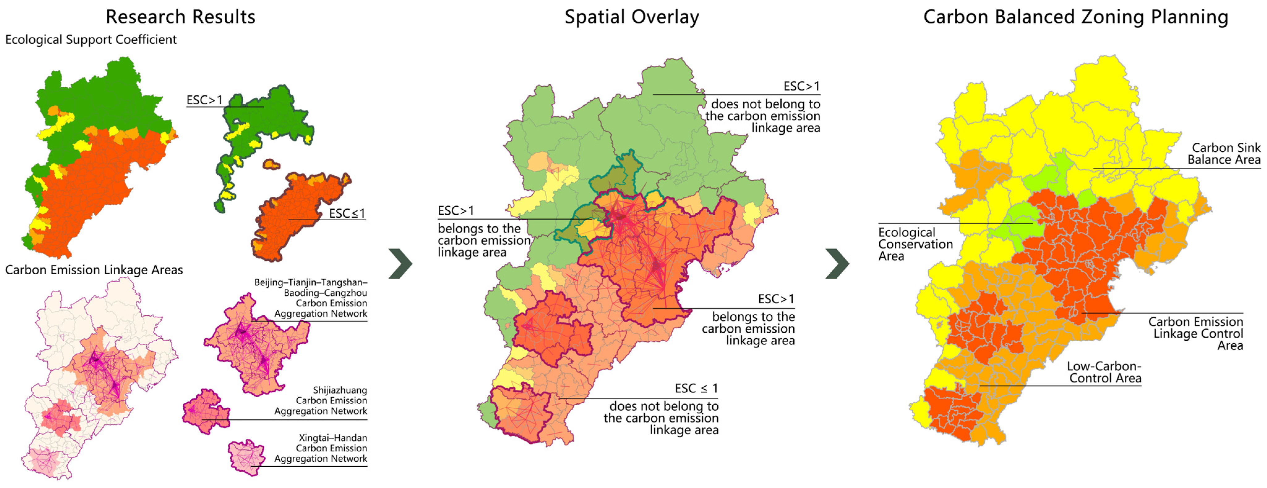
Based on the simulation results of land use under the future LCD scenario, a carbon balance zoning plan for the BTH region in 2035 was developed. ESC was used to characterize the carbon sink potential of a region, while carbon emission linkage regions were used to characterize the potential for regional collaborative emission reduction. We believe that when ESC > 1, the region exhibits carbon-sink-oriented characteristics; when ESC < 1, the region exhibits carbon-emission-oriented characteristics. When the county is in a carbon emission linkage zone, the correlation between networks is high, making it easy to carry out regional collaborative emission reduction work; when the county is not in the carbon emission linkage zone, the correlation between networks is low, making it difficult to carry out regional collaborative emission reduction work. Utilizing the calculated spatial distribution of ESC and the three major carbon emission linkage zones, we divided the carbon balance zoning according to this standard.

3.4.2. Key Carbon Balance and County Planning

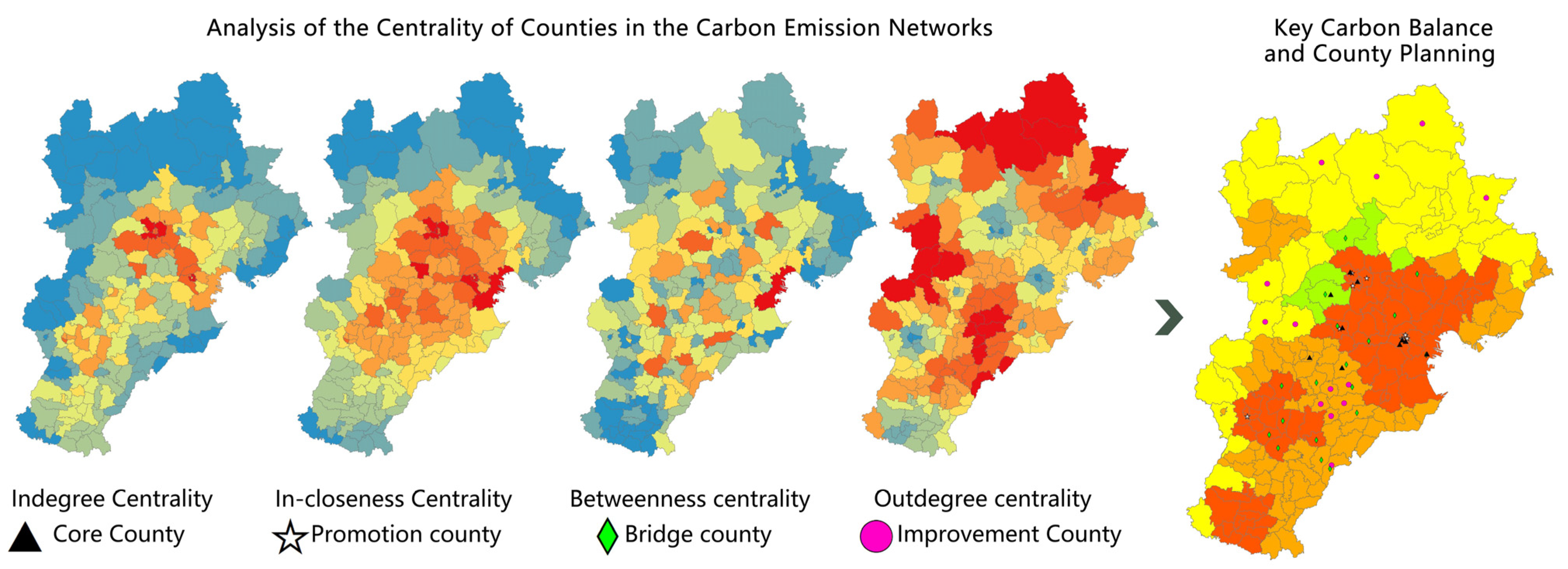
Based on carbon balance zoning planning, the centrality of each county was calculated. The study identified the characteristics of each county in the carbon emission network. Building upon the centrality analysis of each county within the carbon emission network outlined in Section 3.3, four key counties were determined based on the scores of urban agglomerations in the above four indicators: core county, promotion county, bridge county, and improvement county. Among them, counties with higher indegree centrality were designated as core counties, counties with higher in-closeness centrality were designated as promotion counties, counties with higher betweenness centrality were designated as bridge counties, and counties with higher outdegree centrality were designated as improvement counties.

4. Results

4.1. Multi-Scenario Carbon Emission Analysis of the BTH Urban Agglomeration in 2035

4.1.1. Simulation Accuracy Verification

Ensuring the precision of land use model simulation, according to BTH land use in 2010 and 2015, we conducted simulations and compared the expected results of land use in 2020 with the real land use distribution in the same year. The results are displayed in Table 4. Regarding the accuracy validation of the PLUS model, the kappa coefficient stood at 0.9149, with the overall simulation accuracy reaching 0.9402. This outcome indicates that the land use predictions generated by the model in this study had high accuracy [27,40]. Consequently, the model could be extended for simulating land use types and their distributions in 2035 in future studies.

4.1.2. Land Use Distribution Pattern

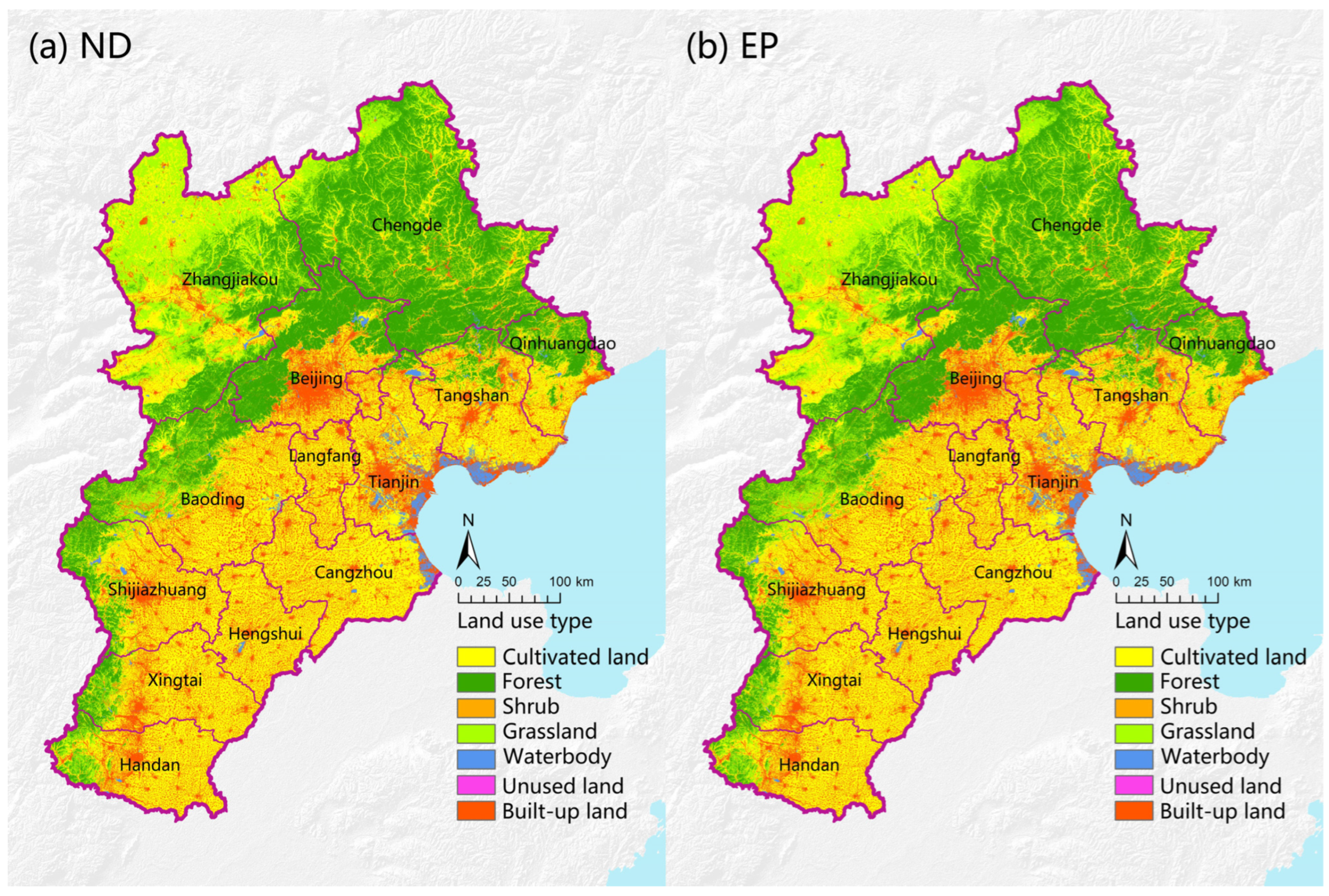
The land use distribution results for 2035 under the two scenarios obtained from the simulation are shown in Figure 3 and Table 5. According to the simulation results, in comparison to land use in 2020, forest land, water bodies, and built-up land would continue to increase, while cultivated land, shrub, grassland, and unused land would decrease in 2035 under the ND scenario. Under the EP scenario, in contrast to the ND scenario, built-up land and cultivated land would decrease by 52,284 ha and 175,628 ha, respectively. The area of ecological land (forest land, shrub, and grassland) would increase by 223,247 ha. Therefore, under the constraints of the EP policy, the disorderly expansion of built-up land in the BTH urban agglomeration in 2035 could be effectively restricted, while the area of ecological land could be augmented.

4.1.3. Spatial Distribution of Carbon Emissions

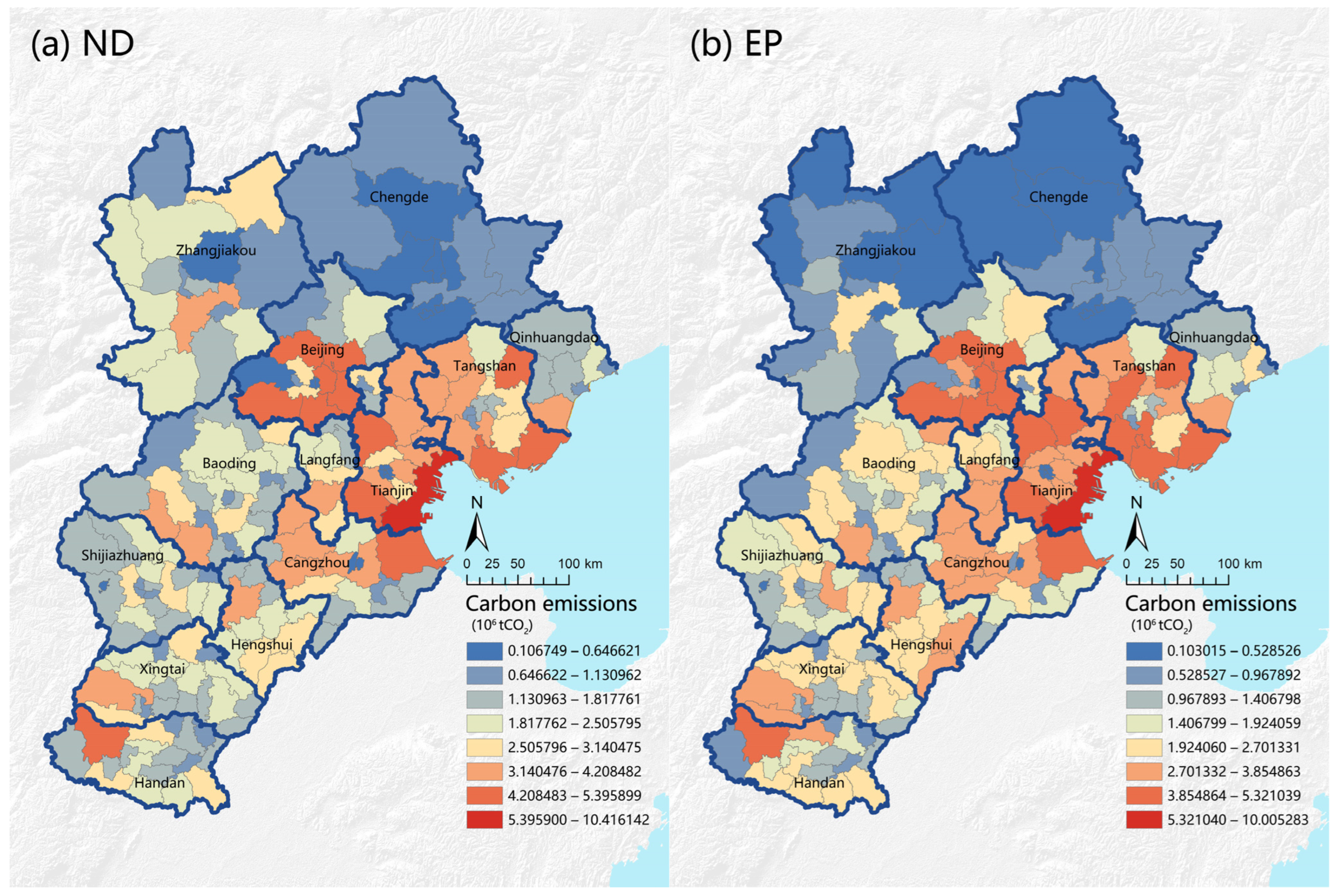
We calculated future carbon emissions in 2035 based on land use patterns under different scenarios (Figure 4 and Table 6). Carbon emissions in 2035 would be 41,408.18 × 104 tons under the ND scenario and 40,764.76 × 104 tons under the EP scenario. In comparison to the ND scenario, the EP scenario would reduce the emission of greenhouse gases by 643.42 × 10⁴ tons. The net carbon sink was larger, leading to lower overall carbon emissions and reduced net carbon emissions.
The spatial distributions of the carbon emissions under the two scenarios exhibited higher concentrations in the central and eastern regions, while they were lower in the western and northern regions. The main areas of carbon emission accumulation included Beijing, Tianjin, Tangshan, Cangzhou, and the Binhai New Area. These accumulation areas are characterized by developed industries, high-density population distributions, highly concentrated distributions of built-up land, and a relatively small proportion of ecological land (forest land and grassland) retaining the same characteristics of carbon emission agglomeration observed in 2020.

4.1.4. Ecological Support Coefficient

ESC was employed to assess the carbon sink capacity under the different development scenarios (Figure 5). The spatial distribution trends of ESC under the two development scenarios were similar, and the overall characteristics were as follows: High ESC values were observed in the northwest, while lower ESC values were noted in the central, southern, and eastern regions. Under the ND scenario, 39 counties had an ESC > 1, accounting for 19.5%. Under the EP scenario, 44 counties had an ESC > 1, accounting for 22%.
We selected the development scenarios with lower carbon emissions and more counties with higher ESC values for the land use prediction results for the LCD scenarios.

4.2. Spatial Correlation Analysis of Carbon Emissions in the BTH Urban Agglomeration under the LCD Scenario

4.2.1. Carbon Emission Network in the BTH Urban Agglomeration

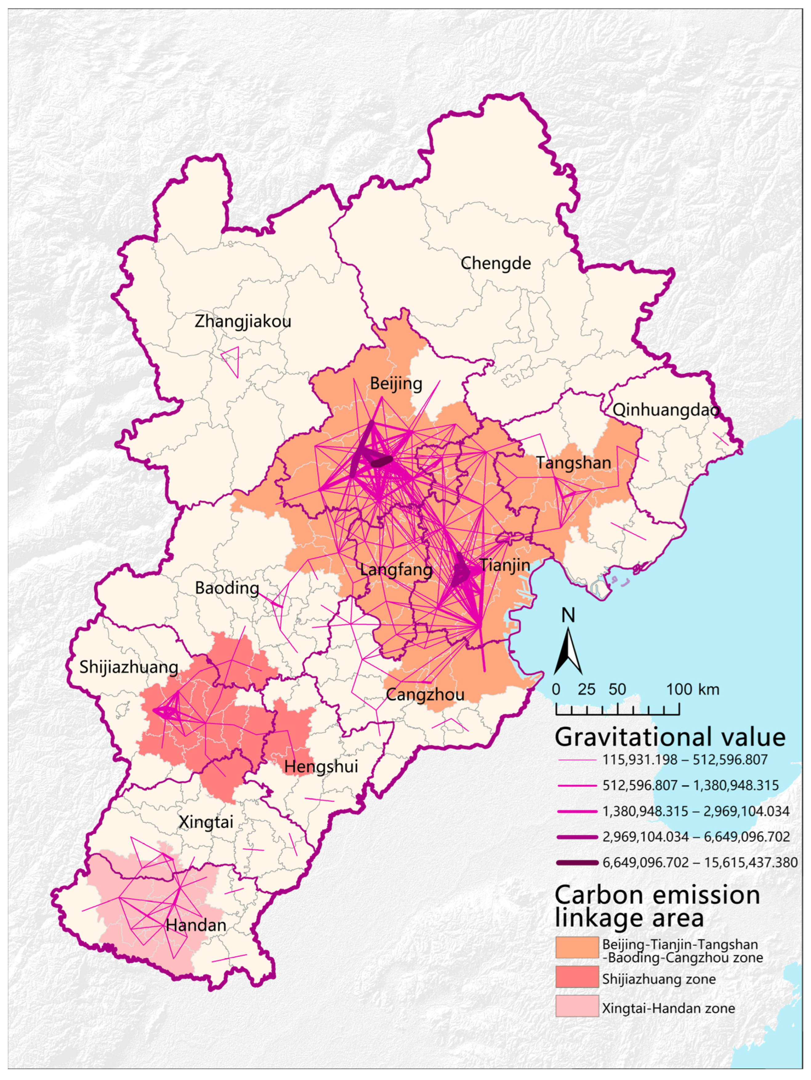
We used the gravity model to draw a carbon emission correlation intensity map of the BTH under the LCD scenario in 2035 (Figure 6). To illustrate the network structure more clearly, we opted to map the carbon emission correlations corresponding to the top 1% of the gravity values [41]. Under the LCD scenario, a distinct spatial correlation pattern of carbon emissions emerged in the BTH region. Beijing, Tianjin, and the neighboring counties of Langfang, Baoding, Tangshan, and Cangzhou in the central area of the study region exhibited close relationships. Conversely, the carbon emission network in the southwestern part of the study area was mainly concentrated in Shijiazhuang and displayed less connectivity with other regions. In the southern region of the study area, the spatial network of carbon emissions was composed mainly of Xingtai and Handan.
According to the gravity values (threshold gravity value = 153,000), the counties with close carbon emission spatial correlations were clustered. We obtained the linkage areas of carbon emissions. Under the LCD scenario, in 2035, the BTH region formed three main groups of carbon emission spatial correlation networks: (1) the Beijing–Tianjin–Tangshan–Baoding–Cangzhou carbon emission aggregation network, with Beijing and Tianjin serving as the dual core hubs; (2) the Shijiazhuang carbon emission aggregation network, which was concentrated in Shijiazhuang Province; and (3) the Xingtai–Handan carbon emission aggregation network, which was composed primarily of Xingtai and Handan. These three carbon emission networks were grouped into three carbon emission linkage areas.

4.2.2. Analysis of the Centrality of Counties in the Carbon Emission Networks

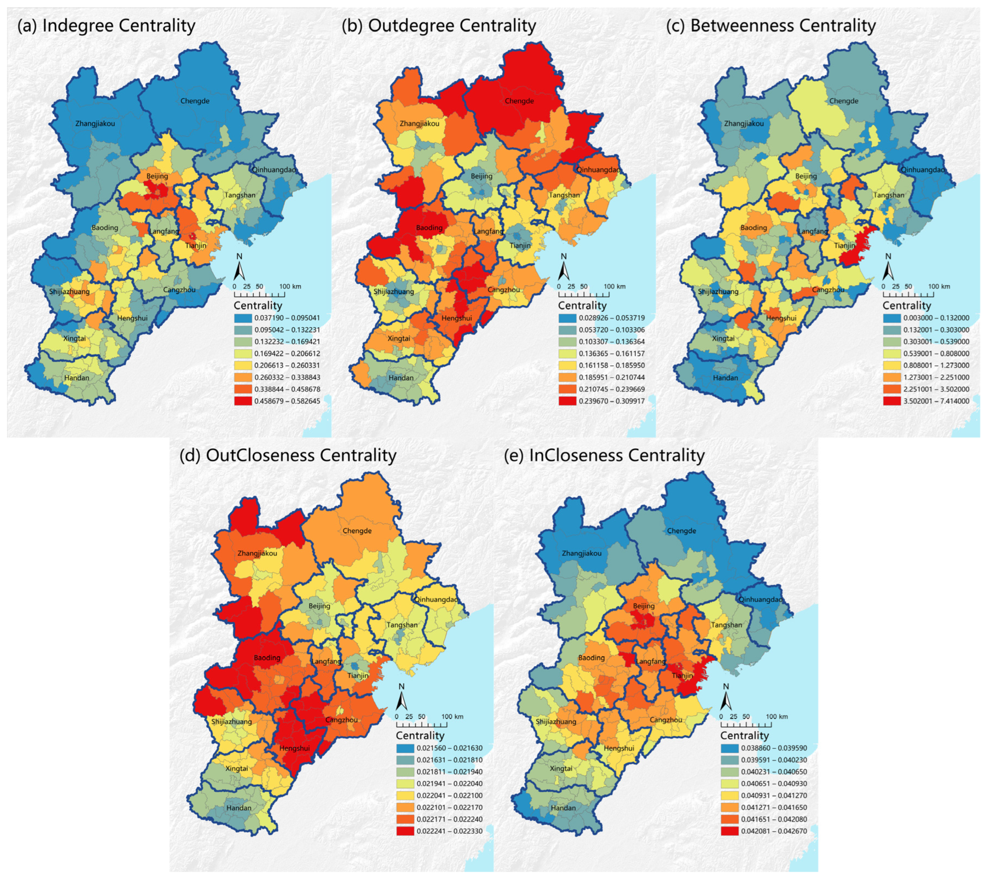
Analyzing and visualizing the centrality of the counties in the networks further clarifies the key counties in the carbon emission networks in the BTH urban agglomeration and offers practical guidance for subsequent planning (Figure 7). The number of counties with the top 10% of the centrality in each city is shown in Table 7. In the centrality evaluation, the counties in Beijing, Tianjin, Baoding, Hengshui, and Cangzhou ranked relatively high, including 46 counties with characteristic nodes. The spatial correlation network of the carbon emissions in the BTH region was centered on the counties included in these cities, which had a significant impact on the spatial spillover of the carbon emissions in urban agglomerations.

4.3. Carbon Balance Planning for the BTH Urban Agglomeration in 2035 under the LCD Scenario

Based on the multi-scenario carbon emission simulation, we selected the EP scenario with lower carbon emissions and more counties with high ESC values as the LCD scenario for the BTH urban agglomeration in 2035. Utilizing the ESC analysis, carbon emission spatial network characteristics, and network centrality of each county under this scenario, we formulated low-carbon-oriented carbon balance zoning planning and carbon balance key county planning.

4.3.1. Carbon Balance Zoning Planning

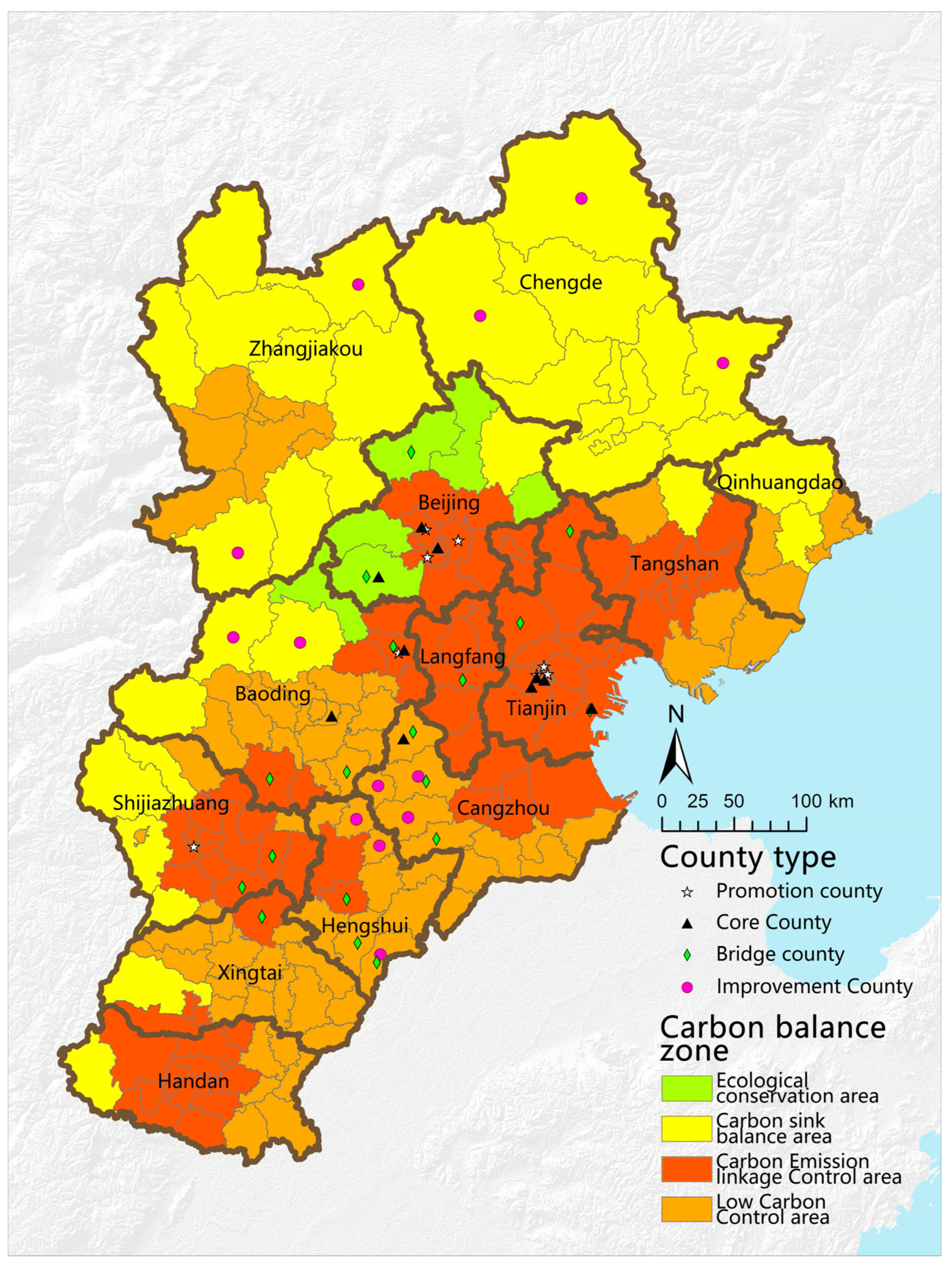
The carbon balance zoning planning was based mainly on the ESC results discussed in Section 4.1.4 and the carbon emission linkage area summarized in the carbon emission network within the urban agglomeration discussed in Section 4.2.1. According to the planning method of carbon balance zoning plan in Section 3.4.1, we divided the zones into four types of zones, and the division process is shown in Figure 8. We divided the BTH urban agglomeration into 33 carbon sink balance areas, six ecological conservation areas, 88 carbon emission linkage control areas, and 74 low-carbon control areas (Table 8).

4.3.2. Key Carbon Balance and County Planning

Based on the centrality analysis of each county in the carbon emission network described in Section 4.2.2, we divided four types of counties according to the planning method of Key Carbon Balance and County Planning in Section 3.4.2. The division process is shown in Figure 9. Based on indegree centrality, outdegree centrality, in-closeness centrality, and betweenness centrality, we identified four types of key counties: core counties, promotion counties, bridge counties, and improvement counties (Table 9 and Figure 10).

5. Discussion

5.1. Multi-Scenario Simulation of Land Use

By setting different constraints, we conducted simulations of the land use patterns within the BTH urban agglomeration in 2035 under different scenarios. In comparison to the ND scenario, the EP scenario saw a transformation of built-up land in Zhangjiakou and Baoding into forest land and grassland, leading to an increase in their carbon sinks and a reduction in their carbon emissions. In addition, under the EP scenario, carbon emissions were low, and the counties with ESC > 1 accounted for a higher percentage of these counties. Carbon emissions in Zhangjiakou and Hengshui decreased significantly. The ecological carrying capacity of the western region of Zhangjiakou improved, transforming from a low-carbon-emission contribution and low-carbon-sink contribution area to a low-carbon-sink contribution and high-carbon-sink contribution area. After comparing the two simulated scenarios, it is evident that the EP scenario imposed stricter limitations on the expansion of built-up land; retained more ecological land, including forest land, shrub, and grassland; produced fewer carbon emissions; eased the problem of the gathering situation of high-carbon-emission areas in spatial patterns, and had stronger carbon sink benefits and ecological benefits. Therefore, we selected the EP scenario as the prediction result for the LCD scenario in the BTH in 2035 for further research and analysis. These research findings demonstrate that through the preservation of ecological functional spaces, controlling unplanned construction land expansion, and execution of policies promoting low-carbon environmental protection development, it is possible to effectively decrease carbon emission intensity and enhance regional carbon sink efficiency. In future planning and construction, these cities will be more conducive to carrying out EP planning actions and maintaining the carbon sequestration benefits of existing forests and grasslands.
We found that carbon emissions were concentrated primarily in the central and eastern counties of the BTH urban agglomeration under the LCD scenario. These findings align with earlier research [42,43]. The ecological support coefficient exhibited higher values in the northwestern region and lower values in the central, southern, and eastern regions. The distribution trend of the overall evaluation results was consistent with the results of a previous study [41], but there were some differences in the distribution of the counties with an ESC < 1. Zhang et al. used the Comprehensive Environmental Data Archive’s (CEDA) database as the source of carbon emission data to calculate the ESCs of Beijing, Tianjin, and Hebei from 2005 to 2017. In this study, we calculated carbon emissions by setting multiple development scenarios, which was more conducive to evaluating carbon balance under different development scenarios and providing suggestions for the zoning planning of low-carbon transformation and development in BTH urban agglomerations.

5.2. Characteristics of Carbon Emission Spatial Networks

In this study, we utilized SNA to analyze the carbon emission network of the BTH urban agglomeration. The use of SNA to analyze the spatial association of carbon emissions can break through traditional geographic restrictions and identify the intricate spatial network connections in each region [19]. The spatial connections of carbon emissions revealed a network structure with Beijing, Tianjin, Tangshan, Baoding, and Cangzhou at its core, alongside clusters located in Shijiazhuang, as well as in Xingtai and Handan. The spatial arrangement of this clustering aligned with findings from prior research [41]. This network of carbon emission spatial clusters exhibited denser connections compared to other urban areas. The collaborative ability of carbon emission networks could be expressed by the number of network connections. Clustered areas with a large number of connections had stronger collaborative capabilities. Further analysis of typical cities that share the characteristics of this network, as well as exploration of the degree of centralization and its characteristics, could help identify the factors that affect the coordinated emission reduction of urban agglomerations. As a result, it would be possible to better formulate low-carbon plans with different goal orientations based on these characteristics.
The centrality degree indicated the crucial role of the nodes within the network. The top 10% of counties in terms of indegree centrality were located mainly in Beijing and Tianjin, where the economy is more developed. These counties had the following characteristics: they undertook a large number of external carbon emission relationships, their industrial structure was more advanced, and their dependence on basic raw materials and energy imports was strong. Furthermore, these counties reside within the core of the spatial network of carbon emissions, situated centrally within the Beijing–Tianjin–Tangshan–Baoding–Cangzhou carbon emission aggregation network. These findings indicate that augmenting the node count in counties in terms of indegree centrality helped promote carbon emission network collaboration. The focus of coordinating carbon emission networks should be on counties with high indegree centrality. The top 10% of the counties in terms of outdegree centrality were all located in Hebei, and these counties had small carbon emissions and strong ecological conservation functions. This result may have been due to the ecological resource advantages of these counties, but the technology level was low and the energy utilization rate was low. Although the core position of the network in these counties was higher than that of other resource-based cities with better ecological benefits, it was still in the middle to low end of the value range in the carbon emission network. These results prove that remote geographical locations, underdeveloped economies, and population levels acted as impediments to the coordinated development of carbon emission networks. Therefore, special consideration should be given to these counties when devising policies, given their relatively passive position in the carbon emission network. As it would be difficult for these counties to achieve positive cooperative effects, more policy support should be given to them.
The closeness of centrality primarily characterized the spatial transfer distance of carbon emissions from counties and determined whether or not carbon transfer links with other counties could be produced more quickly. The top 10% of counties with in-closeness centrality are located in Beijing, Tianjin, and Baoding. These counties shared the following characteristics: they were highly involved in the spatial network of carbon emission integration and established extensive carbon emission links with the surrounding counties, thus becoming central actors in the network. It remains crucial to enhance the connection between hub cities and surrounding cities, enhance their communication, and enhance the synergy of carbon emission networks, thus enabling them to quickly take advantage of regional linkage mechanisms. The top 10% of counties with out-closeness centrality were concentrated in Hengshui, Baoding, and Cangzhou in Hebei Province. These counties occupied a subordinate position in the network and were easily influenced by other regions to make corresponding changes.
Betweenness centrality represented the communication function of one county with other counties. The top 10% of counties are located primarily in Baoding, Beijing, Cangzhou, Hengshui, and Tianjin. The distribution of these counties was relatively scattered and these counties were located in the outskirts areas of key cities. Counties with higher betweenness centrality were more likely to establish carbon emission networks, which meant that carbon emissions between provinces could be exchanged mainly through these cities. This result proved that enhancing the centrality of betweenness could strengthen the transfer of carbon emissions between provinces and promote regional collaboration in carbon emission networks. The counties with high betweenness centrality formed the central relationships connecting surrounding counties, served as good communication bridges, and held great significance in improving the carbon emission network structure.
In summary, fostering collaboration within the carbon emission network in the BTH urban agglomeration requires boosting the centrality of county nodes and internal connectivity. In counties with higher centrality of entry, key policies should be implemented to increase foreign exchange and reduce emissions. Cities with higher inward proximity should be used as policy pilots to strengthen the connections between counties with higher centrality of intermediaries to drive carbon exchange between provinces. Counties with higher centrality of entry should be given more policy assistance. To optimize coordinated regional emission reduction planning, it is essential to comprehensively manage the spatial structure characteristics of urban agglomerations, regulate the association mode, internal groups, and regional status of carbon emissions, and align with the principles of social and economic development [18].

5.3. Recommendations for Key Areas for the Implementation of Emission Peak and Carbon Neutrality Projects

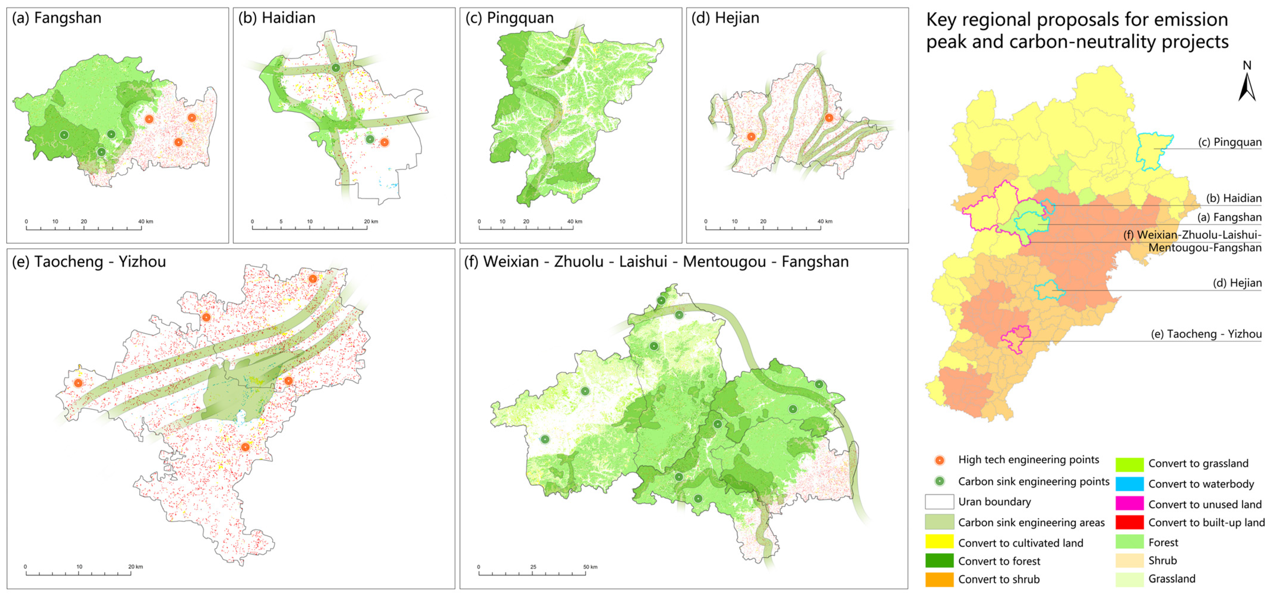
In crafting and executing carbon emission reduction policies, our attention was directed towards the spatial interconnection impact of carbon emissions within the urban agglomeration. We devised a low-carbon-centric carbon balance zoning strategy, leveraging insights from the ESC, spatial network properties of carbon emissions, and network centrality assessment. On this basis, we could further adopt differentiated development strategies for different counties according to the specifics of carbon balance zoning across various regions of the BTH and the functions of key counties in carbon balance. Taking four characteristic counties and two groups of cross-regional cooperation counties as examples, we propose the suggestions given in Table 10 and shown in Figure 11.
The Fangshan District, located in Beijing, is in the ecological conservation area and undertakes the functions of promoting counties and bridge counties. The eastern part of the region is projected to experience a rise in built-up land, while the western part is anticipated to witness an expansion of forest land and grassland. In terms of carbon reduction, we should concentrate on the construction of three high-tech groups in the east and advocate for the development direction of low carbon. To foster compact urban development, efforts will be intensified to promote the construction of bus lanes and dedicated roads [44,45,46]. In terms of increasing foreign exchange, we should construct a recreational and cultural green belt in the plain area [47,48,49].
The Haidian District, located in Beijing, is in the carbon emission linkage control area and serves the functions of core counties and promotion counties. In the forthcoming years, the northern region is expected to witness an augmentation in both built-up and cultivated land, while forest land is projected to expand in the northwest. For carbon reduction endeavors, our focal point should center on Zhongguancun Science City situated in the southern region. It will spearhead the synchronized advancement of low-carbon technology across the carbon emission linkage area [50,51,52] and promote active and public transportation by improving street connectivity [53,54,55]. In terms of increasing sinks, in the future, we should establish the ecological barrier of Xishan Mountain in the northwest as the core position [56,57,58].
Pingquan City, located in Chengde, is in the carbon sink balance area and serves as an improvement county. In the forthcoming years, we anticipate a rise in forest land, grassland, and cultivated land across the entire region. It is crucial to take advantage of these additional regional ecological benefits. In terms of carbon reduction, we should strengthen Pingquan’s support of Beijing’s noncapital functions and actively accept carbon emission spillover within the Beijing–Tianjin region [59,60,61]. In terms of increasing sinks, we should cooperate with the BTH and Liaoning–Inner Mongolia regions to carry out ecological protection [62,63,64,65].
Hejian City, located in Cangzhou, is in the low-carbon control area and serves as an improvement country and bridge country. In the future, there will be a trend of growth in both built-up and cultivated land across the entire region. Therefore, it is essential to prioritize efforts towards promoting carbon reduction initiatives. In terms of carbon reduction, we should decrease reliance on fossil fuels while concurrently elevating the utilization of nuclear and renewable energy sources [66,67]. To augment sinks, it is imperative to establish an ecological security pattern grounded in agriculture, forestry, and water networks. Improve agricultural technology [68], advocate for improving the dietary structure of residents [69,70,71], and reduce the indiscriminate use of fertilizers, organic fertilizers, and chemical fertilizers [72].
The Taocheng District and Jizhou District, located in Hengshui, are in the carbon emission linkage control area and the low-carbon control area, respectively, and serve as bridge counties. In the future, there will be a surge in built-up land on the periphery of the region and an expansion of water bodies in the central area and cultivated land. To advance carbon reduction, fostering interregional collaboration and establishing a national demonstration zone for the conversion of scientific and technological advancements in the southern part of Beijing is crucial [73,74]. We should conform to the expansion trend of the central waterbody in the aspect of increasing the sinks and should carry out ecological restoration in the Fuyang River water ecological comprehensive renovation area around the regional central Hengshui Lake National Nature Reserve [75,76]. We should also promote scientific planning and the construction of tourist areas [77,78].
Yu County and Zhuolu County are located in Zhangjiakou, Laishui County is located in Baoding, and the Mentougou District and Fangshan District are located in Beijing. These counties are in the carbon sink balance area and ecological conservation area. In the future, they will follow a trend of increasing forest land, grassland, and cultivated land. In terms of increasing sinks, we should establish a way of putting regional coordinated ecological restoration planning into action; take advantage of the characteristic county role of bridge, promotion, and improvement counties [79,80]; carry out industry structure adjustment; and coordinate the implementation of emission peak and carbon neutrality policy projects. For the important nature reserves, we should carry out regional coordinated habitat protection optimization and ecological corridor construction. We should also increase the number of nature reserves [81,82].

5.4. A Low-Carbon-Oriented Urban Agglomeration Planning Framework

Numerous studies have consistently demonstrated the pivotal role of regional spatial planning in mitigating regional carbon emissions and attaining climate objectives [83,84,85]. First, spatial planning is comprehensive and can regulate the spatial division of urban agglomerations on a macroscopic scale [86]. Second, spatial planning helps determine the characteristics of cities and formulate differentiated development policies based on the social and economic disparities within the urban agglomeration [87]. Additionally, spatial planning assists in reorganizing spatial relationships within the region, ensuring the balanced and coordinated development of spaces, including residential, commercial, transportation, service, and ecological areas [84]. Given the significance of spatial planning in reducing regional carbon emissions, this study proposes a low-carbon-oriented carbon balance spatial planning method for future urban agglomerations (Figure 12). The overall planning method can be split into four steps:
(1)
By simulating multiple scenarios of land use, we calculated the carbon emissions of urban agglomerations under different scenarios for the future, selected development scenarios align more favorably with low-carbon principles, and optimized the overall spatial scale of regional carbon emissions from the standpoint of urban agglomerations. This approach has been validated in most urban studies [88,89,90], demonstrating that this top-down carbon reduction strategy can be used to adjust future urban land demand, formulate urban expansion plans with minimal ecological losses, and promote compact and green urban development.
(2)
Taking into account the carbon emission characteristics and spatial correlation of urban agglomerations, we utilized carbon balance zoning planning to delineate four distinct carbon balance-oriented zones at the internal spatial correlation level of urban agglomerations. This approach clarifies the spatial development pattern of carbon emissions within urban agglomerations and addresses the question of how to perceive spatial carbon effects. Regional planning with different orientations helps divide the “zoning entities” under the concept of functional control of the main body. The “zoning” control emphasizes respecting and balancing the different roles played by different zoning entities in regulating regional carbon balance, to better protect ecological space and coordinate urban spatial development [43,91].
(3)
Through the analysis of individual network characteristics in social network analysis, we developed the key carbon balance and county planning based on the centrality indicators of each county and analyzed their position within the carbon emission network. Clear guidance and development goals for carbon reduction actions in different counties were established. In the field of urban planning, the literature has shown that governments and policymakers worldwide intend to utilize various data and measurement methods to ascertain urban characteristics; summarize regional political, economic, and social characteristics; and plan cities based on these factors to better address the needs of people regarding housing, economic opportunities, and social system changes [87].
(4)
Finally, we developed key areas for the implementation of emission peak and carbon neutrality projects by analyzing the land features within the county. By scaling down from the level of urban agglomerations, we analyzed the composition of land parcel elements within the county. By optimizing the structure of industrial land, energy land, ecological land, agricultural land, and transportation land, we further optimized the structure of the carbon-source and carbon-sink land and implemented urban spatial planning accordingly. We guided the practice of county-level urban spatial planning in terms of low-carbon layout, low-carbon industries, low-carbon transportation, low-carbon human settlements, and ecological green spaces to better regulate carbon spatial layout and formulate a carbon intensity design. Urban and transportation planners have conducted various studies on achieving carbon neutrality goals at this level, and combined with the low-carbon planning tasks of county-level urban spaces, they have screened and extracted planning and control elements from both qualitative and quantitative perspectives, and implemented them in practice [45,92,93,94].
In summary, we started from four levels: the overall space of the urban agglomeration, the spatial correlation areas within the urban agglomeration, each county, and the internal land features within the county. We optimized the carbon emission scale through scenario simulation, coordinated the carbon emission spatial development pattern through carbon balance zoning planning, clarified the carbon emission action goals through key carbon balance and county planning, and finally, established key areas for the implementation of emission peak and carbon neutrality projects to regulate the carbon spatial layout and formulate carbon intensity designs in response to the carbon effects of land types, space, urban areas, and spatial elements. By starting from a multi-scale spatial pattern, developing multilevel action plans, constructing a planning policy framework, and integrating carbon reduction and sink enhancement goals into multilevel and multi-class spatial planning, we aim to achieve the leading, comprehensive, and fundamental nature of regional carbon reduction policies, thereby more widely guiding their application in major urban agglomerations around the world.

5.5. Limitations

While this study examined the interplay between future land use changes and social networks within spatial planning, it is important to acknowledge certain limitations. Specifically, during the process of simulating land use carbon emissions, variations in carbon emission intensities across different land use types and years might have existed, particularly concerning built-up land. In the process of comparing future development scenarios, however, this research method can still effectively screen more low-carbon simulation results, and these results can be used as an optimization guide to build a carbon-neutral territorial spatial pattern system. Additionally, although this study developed a multi-scale and multilevel research framework through calculations and references to articles from various planning fields worldwide, it has not yet been validated through virtual simulation models to evaluate the feasibility of planning policies. In future research, it would be valuable to conduct additional evaluation studies to assess the effectiveness of carbon emission reduction planning initiatives.

6. Conclusions and Contribution

In this study, we focused on the urban agglomeration comprising BTH county-level units as our research subject. We established a theoretical framework for carbon balance planning from the standpoint of low-carbon development. Future land use patterns were simulated under different development scenarios, and we selected low-carbon-oriented development models. On this basis, we introduced the socioeconomic factors of the urban agglomeration and constructed a spatial association network of the carbon emissions in the BTH urban agglomeration under LCD scenarios. Based on the spatial network characteristics and centrality characteristics, we carried out carbon balance zoning planning, clarified the functional characteristics of the different zoning areas and key counties, delineated the key areas for carbon neutrality projects, and proposed suggestions. The primary findings of the research are outlined below:
  • We simulated land use patterns under the ND and EP scenarios in the BTH in 2035. Carbon emissions from land use under the EP scenario decreased by 643.42 × 10⁴ t. The spatial distribution was characterized by lower carbon emission and higher ESC values in the northwest and higher carbon emissions and lower ESC values in the central, southern, and eastern regions. We selected the EP scenario as the prediction result of the LCD scenario for the BTH in 2035 for further analysis;
  • Carbon emissions within the BTH were closely related, forming three major carbon emission linkage areas: Beijing–Tianjin–Tangshan–Baoding–Cangzhou, Shijiazhuang, and Xingtai–Handan. The counties of Beijing, Tianjin, Baoding, Hengshui, and Cangzhou and other cities in the central region had different levels of individual centrality.
  • Based on the characteristics of the ESC and carbon emission network, we formulated a carbon balance zoning plan for the BTH urban agglomeration in 2035 under the LCD scenario. The urban agglomeration underwent division into four areas: ecological conservation, carbon sink balance, carbon emission control, and low-carbon control areas. Furthermore, we selected the core counties, promotion counties, bridge counties, and improvement counties according to the characteristics of the network centrality. We pinpointed critical zones for the execution of emission peak and carbon neutrality projects within the distinctive counties. Furthermore, we put forth tailored recommendations aimed at mitigating carbon emissions and augmenting carbon sinks based on the prevailing characteristics of the study area.

Author Contributions

Conceptualization, H.L. and Y.L. (Yang Liu); methodology, H.L. and Y.L. (Yang Liu); software, H.L. and Y.L. (Yixiao Li); validation, H.L. and X.L.; formal analysis, H.L. and S.Y.; investigation, H.L.; resources, H.L. and X.Z.; data curation, H.L.; writing—original draft preparation, H.L.; writing—review and editing, H.L. and Y.L. (Yang Liu); visualization, H.L.; supervision, X.Z.; project administration, Y.L. (Yang Liu); funding acquisition, X.Z. All authors have read and agreed to the published version of the manuscript.

Funding

We thank the National Natural Science Foundation of China (grant numbers 32371643) for the financial support of this research.

Data Availability Statement

The original contributions presented in the study are included in the article, further inquiries can be directed to the corresponding author.

Conflicts of Interest

The authors declare no conflicts of interest.

References

  1. Masson-Delmotte, V.; Zhai, P.; Pirani, A.; Connors, S.L.; Péan, C.; Berger, S.; Caud, N.; Chen, Y.; Goldfarb, L.; Gomis, M. Climate change 2021: The physical science basis. In Contribution of Working Group I to the Sixth Assessment Report of the Intergovernmental Panel on Climate Change; 2021; Volume 2, p. 2391. Available online: https://www.ipcc.ch/report/ar6/wg1/ (accessed on 15 April 2024).
  2. Pachauri, R.K.; Gomez-Echeverri, L.; Riahi, K. Synthesis Report: Summary for Policy Makers, 2014; pp. 1–30.
  3. Meng, L.; Graus, W.; Worrell, E.; Huang, B. Estimating CO2 (carbon dioxide) emissions at urban scales by DMSP/OLS (Defense Meteorological Satellite Program’s Operational Linescan System) nighttime light imagery: Methodological challenges and a case study for China. Energy 2014, 71, 468–478. [Google Scholar] [CrossRef]
  4. Li, L.; Ma, S.; Zheng, Y.; Xiao, X. Integrated regional development: Comparison of urban agglomeration policies in China. Land Use Policy 2022, 114, 105939. [Google Scholar] [CrossRef]
  5. Lin, Q.; Zhang, L.; Qiu, B.; Zhao, Y.; Wei, C. Spatiotemporal analysis of land-use patterns on carbon emissions in China. Land 2021, 10, 141. [Google Scholar] [CrossRef]
  6. Li, W.; Ciais, P.; Peng, S.; Yue, C.; Wang, Y.; Thurner, M.; Saatchi, S.S.; Arneth, A.; Avitabile, V.; Carvalhais, N. Land-use and land-cover change carbon emissions between 1901 and 2012 constrained by biomass observations. Biogeosciences 2017, 14, 5053–5067. [Google Scholar] [CrossRef]
  7. Zhao, J.; Cohen, J.B.; Chen, Y.; Cui, W.; Cao, Q.; Yang, T.; Li, G. High-resolution spatiotemporal patterns of China’s FFCO2 emissions under the impact of LUCC from 2000 to 2015. Environ. Res. Lett. 2020, 15, 044007. [Google Scholar] [CrossRef]
  8. Jing, Q.; Bai, H.; Luo, W.; Cai, B.; Xu, H. A top-bottom method for city-scale energy-related CO2 emissions estimation: A case study of 41 Chinese cities. J. Clean. Prod. 2018, 202, 444–455. [Google Scholar] [CrossRef]
  9. Yang, S.; Fu, W.; Hu, S.; Ran, P. Watershed carbon compensation based on land use change: Evidence from the Yangtze River Economic Belt. Habitat Int. 2022, 126, 102613. [Google Scholar] [CrossRef]
  10. Basse, R.M.; Omrani, H.; Charif, O.; Gerber, P.; Bódis, K. Land use changes modelling using advanced methods: Cellular automata and artificial neural networks. The spatial and explicit representation of land cover dynamics at the cross-border region scale. Appl. Geogr. 2014, 53, 160–171. [Google Scholar] [CrossRef]
  11. Ku, C.-A. Incorporating spatial regression model into cellular automata for simulating land use change. Appl. Geogr. 2016, 69, 1–9. [Google Scholar] [CrossRef]
  12. Verburg, P.H.; Soepboer, W.; Veldkamp, A.; Limpiada, R.; Espaldon, V.; Mastura, S.S. Modeling the spatial dynamics of regional land use: The CLUE-S model. Environ. Manag. 2002, 30, 391–405. [Google Scholar] [CrossRef]
  13. Liu, X.; Liang, X.; Li, X.; Xu, X.; Ou, J.; Chen, Y.; Li, S.; Wang, S.; Pei, F. A future land use simulation model (FLUS) for simulating multiple land use scenarios by coupling human and natural effects. Landsc. Urban Plan. 2017, 168, 94–116. [Google Scholar] [CrossRef]
  14. Xie, L.; Bai, Z.; Yang, B.; Fu, S. Simulation Analysis of Land-Use Pattern Evolution and Valuation of Terrestrial Ecosystem Carbon Storage of Changzhi City, China. Land 2022, 11, 1270. [Google Scholar] [CrossRef]
  15. Dong, L.; Liang, H.; Zhang, L.; Liu, Z.; Gao, Z.; Hu, M. Highlighting regional eco-industrial development: Life cycle benefits of an urban industrial symbiosis and implications in China. Ecol. Model. 2017, 361, 164–176. [Google Scholar] [CrossRef]
  16. Qian, Y.; Wang, H.; Wu, J. Spatiotemporal association of carbon dioxide emissions in China’s urban agglomerations. J. Environ. Manag. 2022, 323, 116109. [Google Scholar] [CrossRef] [PubMed]
  17. Shen, W.; Liang, H.; Dong, L.; Ren, J.; Wang, G. Synergistic CO2 reduction effects in Chinese urban agglomerations: Perspectives from social network analysis. Sci. Total Environ. 2021, 798, 149352. [Google Scholar] [CrossRef]
  18. Dong, J.; Li, C. Structure characteristics and influencing factors of China’s carbon emission spatial correlation network: A study based on the dimension of urban agglomerations. Sci. Total Environ. 2022, 853, 158613. [Google Scholar] [CrossRef]
  19. Yu, Z.; Chen, L.; Tong, H.; Chen, L.; Zhang, T.; Li, L.; Yuan, L.; Xiao, J.; Wu, R.; Bai, L. Spatial correlations of land-use carbon emissions in the Yangtze River Delta region: A perspective from social network analysis. Ecol. Indic. 2022, 142, 109147. [Google Scholar] [CrossRef]
  20. Wang, C.; Zhan, J.; Zhang, F.; Liu, W.; Twumasi-Ankrah, M.J. Analysis of urban carbon balance based on land use dynamics in the Beijing-Tianjin-Hebei region, China. J. Clean. Prod. 2021, 281, 125138. [Google Scholar] [CrossRef]
  21. Hurlimann, A.; Moosavi, S.; Browne, G.R. Urban planning policy must do more to integrate climate change adaptation and mitigation actions. Land Use Policy 2021, 101, 105188. [Google Scholar] [CrossRef]
  22. Haas, J.; Ban, Y. Urban growth and environmental impacts in jing-jin-ji, the yangtze, river delta and the pearl river delta. Int. J. Appl. Earth Obs. Geoinf. 2014, 30, 42–55. [Google Scholar] [CrossRef]
  23. Gu, R.; Li, C.; Li, D.; Yang, Y.; Gu, S. The impact of rationalization and upgrading of industrial structure on carbon emissions in the Beijing-Tianjin-Hebei urban agglomeration. Int. J. Environ. Res. Public Health 2022, 19, 7997. [Google Scholar] [CrossRef] [PubMed]
  24. Yang, J.; Huang, X. The 30 m annual land cover dataset and its dynamics in China from 1990 to 2019. Earth Syst. Sci. Data 2021, 13, 3907–3925. [Google Scholar] [CrossRef]
  25. Zhong, X.; Yan, Q.; Li, G. Development of the Long Time Series Nighttime Light Dataset of China (2000–2020). J. Glob. Chang. Data Discov. 2022, 3, 420–428. [Google Scholar]
  26. Li, X.; Liu, Z.; Li, S.; Li, Y. Multi-scenario simulation analysis of land use impacts on habitat quality in Tianjin based on the PLUS model coupled with the InVEST model. Sustainability 2022, 14, 6923. [Google Scholar] [CrossRef]
  27. Luo, S.; Hu, X.; Sun, Y.; Yan, C.; Zhang, X. Multi-scenario land use change and its impact on carbon storage based on coupled Plus-Invest model. Chin. J. Eco-Agric. 2023, 31, 300–314. [Google Scholar]
  28. Cui, X.; Wei, X.; Liu, W.; Zhang, F.; Li, Z. Spatial and temporal analysis of carbon sources and sinks through land use/cover changes in the Beijing-Tianjin-Hebei urban agglomeration region. Phys. Chem. Earth Parts A/B/C 2019, 110, 61–70. [Google Scholar] [CrossRef]
  29. Fang, J.; Guo, Z.; Piao, S.; Chen, A. Terrestrial vegetation carbon sinks in China, 1981–2000. Sci. China Ser. D Earth Sci. 2007, 50, 1341–1350. [Google Scholar] [CrossRef]
  30. Liu, C.; Xu, R.; Xu, K.; Lin, Y.; Cao, Y. Carbon Emission Effects of Land Use in Chaobai River Region of Beijing–Tianjin–Hebei, China. Land 2023, 12, 1168. [Google Scholar] [CrossRef]
  31. She, W.; Wu, Y.; Huang, H.; Chen, Z.; Cui, G.; Zheng, H.; Guan, C.; Chen, F. Integrative analysis of carbon structure and carbon sink function for major crop production in China’s typical agriculture regions. J. Clean. Prod. 2017, 162, 702–708. [Google Scholar] [CrossRef]
  32. Tang, X.; Zhao, X.; Bai, Y.; Tang, Z.; Wang, W.; Zhao, Y.; Wan, H.; Xie, Z.; Shi, X.; Wu, B. Carbon pools in China’s terrestrial ecosystems: New estimates based on an intensive field survey. Proc. Natl. Acad. Sci. USA 2018, 115, 4021–4026. [Google Scholar] [CrossRef]
  33. Yan, H.; Guo, X.; Zhao, S.; Yang, H. Variation of net carbon emissions from land use change in the Beijing-Tianjin-Hebei region during 1990–2020. Land 2022, 11, 997. [Google Scholar] [CrossRef]
  34. Huang, H.; Zhou, J. Study on the spatial and temporal differentiation pattern of carbon emission and carbon compensation in China’s provincial areas. Sustainability 2022, 14, 7627. [Google Scholar] [CrossRef]
  35. Rong, T.; Zhang, P.; Jing, W.; Zhang, Y.; Li, Y.; Yang, D.; Yang, J.; Chang, H.; Ge, L. Carbon dioxide emissions and their driving forces of land use change based on Economic Contributive Coefficient (ECC) and Ecological Support Coefficient (ESC) in the lower Yellow river region (1995–2018). Energies 2020, 13, 2600. [Google Scholar] [CrossRef]
  36. Wang, F.; Gao, M.; Liu, J.; Fan, W. The spatial network structure of China’s regional carbon emissions and its network effect. Energies 2018, 11, 2706. [Google Scholar] [CrossRef]
  37. Ho, H.-X.T. Forecasting of CO2 emissions, renewable energy consumption and economic growth in vietnam using grey models. In Proceedings of the 2018 4th International Conference on Green Technology and Sustainable Development (GTSD), Ho Chi Minh City, Vietnam, 23–24 November 2018; pp. 452–455. [Google Scholar]
  38. Wang, B.; Ge, Y. Predicting the influence of Guangfo Metro on the economic level of Foshan City Based on the GM (1, 1) model. IOP Conf. Ser. Earth Environ. Sci. 2021, 634, 012013. [Google Scholar] [CrossRef]
  39. Zhao, N.; Liu, Y.; Cao, G.; Samson, E.L.; Zhang, J. Forecasting China’s GDP at the pixel level using nighttime lights time series and population images. GIScience Remote Sens. 2017, 54, 407–425. [Google Scholar] [CrossRef]
  40. Wang, Z.; Li, X.; Mao, Y.; Li, L.; Wang, X.; Lin, Q. Dynamic simulation of land use change and assessment of carbon storage based on climate change scenarios at the city level: A case study of Bortala, China. Ecol. Indic. 2022, 134, 108499. [Google Scholar] [CrossRef]
  41. Zhang, Z.; Zhang, D. Spatial connection of CO2 emission and carbon balance zoning in Beijing Tianjin Hebei counties based on social network analysis. China Environ. Sci. 2023, 43, 2057–2068. [Google Scholar] [CrossRef]
  42. Fu, H.; Zhao, S.; Liao, C. Spatial governance of Beijing-Tianjin-Hebei urban agglomeration towards low-carbon transition. China Agric. Econ. Rev. 2022, 14, 774–798. [Google Scholar] [CrossRef]
  43. Liu, G.; Zhang, F. Land Zoning Management to Achieve Carbon Neutrality: A Case Study of the Beijing–Tianjin–Hebei Urban Agglomeration, China. Land 2022, 11, 551. [Google Scholar] [CrossRef]
  44. Ewing, R.; Cervero, R. “Does compact development make people drive less?” The answer is yes. J. Am. Plan. Assoc. 2017, 83, 19–25. [Google Scholar] [CrossRef]
  45. Gao, S.; Zhang, H. Urban planning for low-carbon sustainable development. Sustain. Comput. Inform. Syst. 2020, 28, 100398. [Google Scholar] [CrossRef]
  46. Malambo, P.; Kengne, A.P.; De Villiers, A.; Lambert, E.V.; Puoane, T. Built environment, selected risk factors and major cardiovascular disease outcomes: A systematic review. PLoS ONE 2016, 11, e0166846. [Google Scholar] [CrossRef] [PubMed]
  47. Bastin, J.-F.; Finegold, Y.; Garcia, C.; Mollicone, D.; Rezende, M.; Routh, D.; Zohner, C.M.; Crowther, T.W. The global tree restoration potential. Science 2019, 365, 76–79. [Google Scholar] [CrossRef] [PubMed]
  48. Yang, J. Strategies for low-carbon green growth and urban management in Korea. J. Urban Manag. 2013, 2, 85–101. [Google Scholar] [CrossRef]
  49. Ye, Y.; Wang, C.; Zhang, Y.; Wu, K.; Wu, Q.; Su, Y. Low-carbon transportation oriented urban spatial structure: Theory, model and case study. Sustainability 2017, 10, 19. [Google Scholar] [CrossRef]
  50. Cifuentes, L.; Borja-Aburto, V.H.; Gouveia, N.; Thurston, G.; Davis, D.L. Assessing the health benefits of urban air pollution reductions associated with climate change mitigation (2000–2020): Santiago, São Paulo, México City, and New York City. Environ. Health Perspect. 2001, 109, 419–425. [Google Scholar]
  51. Dudek, D.; Golub, A.; Strukova, E. Ancillary benefits of reducing greenhouse gas emissions in transitional economies. World Dev. 2003, 31, 1759–1769. [Google Scholar] [CrossRef]
  52. Wang, X.; Smith, K.R. Secondary Benefits of Greenhouse Gas Control: Health Impacts in China. Environ. Sci. Technol. 1999, 33, 3056–3061. [Google Scholar] [CrossRef]
  53. Djurhuus, S.; Hansen, H.S.; Aadahl, M.; Glümer, C. The association between access to public transportation and self-reported active commuting. Int. J. Environ. Res. Public Health 2014, 11, 12632–12651. [Google Scholar] [CrossRef]
  54. Florindo, A.A.; Barrozo, L.V.; Turrell, G.; Barbosa, J.P.d.A.S.; Cabral-Miranda, W.; Cesar, C.L.G.; Goldbaum, M. Cycling for transportation in Sao Paulo City: Associations with bike paths, train and subway stations. Int. J. Environ. Res. Public Health 2018, 15, 562. [Google Scholar] [CrossRef] [PubMed]
  55. Pucher, J.; Dill, J.; Handy, S. Infrastructure, programs, and policies to increase bicycling: An international review. Prev. Med. 2010, 50, S106–S125. [Google Scholar] [CrossRef] [PubMed]
  56. Bustamante, M.M.; Silva, J.S.; Scariot, A.; Sampaio, A.B.; Mascia, D.L.; Garcia, E.; Sano, E.; Fernandes, G.W.; Durigan, G.; Roitman, I. Ecological restoration as a strategy for mitigating and adapting to climate change: Lessons and challenges from Brazil. Mitig. Adapt. Strateg. Glob. Chang. 2019, 24, 1249–1270. [Google Scholar] [CrossRef]
  57. Galatowitsch, S.M. Carbon offsets as ecological restorations. Restor. Ecol. 2009, 17, 563–570. [Google Scholar] [CrossRef]
  58. Lim, C.H.; Lim, B.S.; Kim, A.R.; Kim, D.U.; Seol, J.W.; Pi, J.H.; Lee, H.; Lee, C.S. Climate change adaptation through ecological restoration. In Natural Resources Conservation and Advances for Sustainability; Elsevier: Amsterdam, The Netherlands, 2022; pp. 151–172. [Google Scholar]
  59. Chen, Y. Does a regional greenhouse gas policy make sense? A case study of carbon leakage and emissions spillover. Energy Econ. 2009, 31, 667–675. [Google Scholar] [CrossRef]
  60. Gu, G.; Wang, Z.; Wu, L. Carbon emission reductions under global low-carbon technology transfer and its policy mix with R&D improvement. Energy 2021, 216, 119300. [Google Scholar]
  61. Zhang, Y. Spillover and Feedback Effects in Low Carbon Development; Springer: Singapore; Prime Minister’s Office: Singapore, 2021.
  62. Cao, S.; Li, C. The exploration of concepts and methods for low-carbon eco-city planning. Procedia Environ. Sci. 2011, 5, 199–207. [Google Scholar] [CrossRef]
  63. Li, D.; Fan, K.; Lu, J.; Wu, S.; Xie, X. Research on Spatio-Temporal Pattern Evolution and the Coupling Coordination Relationship of Land-Use Benefit from a Low-Carbon Perspective: A Case Study of Fujian Province. Land 2022, 11, 1498. [Google Scholar] [CrossRef]
  64. Wang, C.; Zhan, J.; Xin, Z. Comparative analysis of urban ecological management models incorporating low-carbon transformation. Technol. Forecast. Soc. Chang. 2020, 159, 120190. [Google Scholar] [CrossRef]
  65. Wang, Z. Coordinated development of regional resources, environment, and economic growth under the background of low-carbon economy. Front. Ecol. Evol. 2023, 11, 1181990. [Google Scholar] [CrossRef]
  66. He, K.; Lei, Y.; Pan, X.; Zhang, Y.; Zhang, Q.; Chen, D. Co-benefits from energy policies in China. Energy 2010, 35, 4265–4272. [Google Scholar] [CrossRef]
  67. Markandya, A.; Armstrong, B.G.; Hales, S.; Chiabai, A.; Criqui, P.; Mima, S.; Tonne, C.; Wilkinson, P. Public health benefits of strategies to reduce greenhouse-gas emissions: Low-carbon electricity generation. Lancet 2009, 374, 2006–2015. [Google Scholar] [CrossRef]
  68. Friel, S.; Dangour, A.D.; Garnett, T.; Lock, K.; Chalabi, Z.; Roberts, I.; Butler, A.; Butler, C.D.; Waage, J.; McMichael, A.J. Public health benefits of strategies to reduce greenhouse-gas emissions: Food and agriculture. Lancet 2009, 374, 2016–2025. [Google Scholar] [CrossRef]
  69. Biesbroek, S.; Bueno-de-Mesquita, H.B.; Peeters, P.H.; Verschuren, W.M.; Van Der Schouw, Y.T.; Kramer, G.F.; Tyszler, M.; Temme, E.H. Reducing our environmental footprint and improving our health: Greenhouse gas emission and land use of usual diet and mortality in EPIC-NL: A prospective cohort study. Environ. Health 2014, 13, 1–9. [Google Scholar] [CrossRef] [PubMed]
  70. Milner, J.; Green, R.; Dangour, A.D.; Haines, A.; Chalabi, Z.; Spadaro, J.; Markandya, A.; Wilkinson, P. Health effects of adopting low greenhouse gas emission diets in the UK. BMJ Open 2015, 5, e007364. [Google Scholar] [CrossRef]
  71. Springmann, M.; Godfray, H.C.J.; Rayner, M.; Scarborough, P. Analysis and valuation of the health and climate change cobenefits of dietary change. Proc. Natl. Acad. Sci. USA 2016, 113, 4146–4151. [Google Scholar] [CrossRef]
  72. Xiong, C.; Wang, G.; Su, W.; Gao, Q. Selecting low-carbon technologies and measures for high agricultural carbon productivity in Taihu Lake Basin, China. Environ. Sci. Pollut. Res. 2021, 28, 49913–49920. [Google Scholar] [CrossRef]
  73. Rogge, K.S.; Pfluger, B.; Geels, F.W. Transformative policy mixes in socio-technical scenarios: The case of the low-carbon transition of the German electricity system (2010–2050). Technol. Forecast. Soc. Chang. 2020, 151, 119259. [Google Scholar] [CrossRef]
  74. Wang, Y.; Ren, H.; Dong, L.; Park, H.-S.; Zhang, Y.; Xu, Y. Smart solutions shape for sustainable low-carbon future: A review on smart cities and industrial parks in China. Technol. Forecast. Soc. Chang. 2019, 144, 103–117. [Google Scholar] [CrossRef]
  75. Cheng, Q.; Su, B.; Tan, J. Developing an evaluation index system for low-carbon tourist attractions in China–A case study examining the Xixi wetland. Tour. Manag. 2013, 36, 314–320. [Google Scholar] [CrossRef]
  76. Cheshmehzangi, A.; Xie, L.; Tan-Mullins, M. The role of international actors in low-carbon transitions of Shenzhen’s International Low Carbon City in China. Cities 2018, 74, 64–74. [Google Scholar] [CrossRef]
  77. Li, J.H.; Sia, R.; Yang, L. Study on low-carbon development in the eco-tourism area: Taking Qinghai Lake of China as an example. Adv. Mater. Res. 2012, 524, 2442–2447. [Google Scholar] [CrossRef]
  78. Qing, L. Study on Poyang Lake Tourism Plan under the Low-Carbon Ecology. Appl. Mech. Mater. 2013, 368, 369–374. [Google Scholar] [CrossRef]
  79. Heinen, D. Growth management for low-carbon development patterns–leverages in state planning enabling legislation. Urban Res. Pract. 2022, 15, 71–93. [Google Scholar] [CrossRef]
  80. Song, Q.; Liu, T.; Qi, Y. Policy innovation in low carbon pilot cities: Lessons learned from China. Urban Clim. 2021, 39, 100936. [Google Scholar] [CrossRef]
  81. Chen, J.; Wang, Z. Low-Carbon Rural Landscape Optimization Strategy Based on Green Infrastructure Evaluation. J. Simul. 2021, 9, 125. [Google Scholar]
  82. Khanna, N.; Fridley, D.; Hong, L. China’s pilot low-carbon city initiative: A comparative assessment of national goals and local plans. Sustain. Cities Soc. 2014, 12, 110–121. [Google Scholar] [CrossRef]
  83. Gao, J.; Kovats, S.; Vardoulakis, S.; Wilkinson, P.; Woodward, A.; Li, J.; Gu, S.; Liu, X.; Wu, H.; Wang, J. Public health co-benefits of greenhouse gas emissions reduction: A systematic review. Sci. Total Environ. 2018, 627, 388–402. [Google Scholar] [CrossRef]
  84. Mueller, N.; Daher, C.; Rojas-Rueda, D.; Delgado, L.; Vicioso, H.; Gascon, M.; Marquet, O.; Vert, C.; Martin, I.; Nieuwenhuijsen, M. Integrating health indicators into urban and transport planning: A narrative literature review and participatory process. Int. J. Hyg. Environ. Health 2021, 235, 113772. [Google Scholar] [CrossRef]
  85. Nieuwenhuijsen, M.J. Urban and transport planning pathways to carbon neutral, liveable and healthy cities; A review of the current evidence. Environ. Int. 2020, 140, 105661. [Google Scholar] [CrossRef]
  86. Biesbroek, G.R.; Swart, R.J.; Van der Knaap, W.G. The mitigation–adaptation dichotomy and the role of spatial planning. Habitat Int. 2009, 33, 230–237. [Google Scholar] [CrossRef]
  87. Wang, S.-H.; Huang, S.-L.; Huang, P.-J. Can spatial planning really mitigate carbon dioxide emissions in urban areas? A case study in Taipei, Taiwan. Landsc. Urban Plan. 2018, 169, 22–36. [Google Scholar] [CrossRef]
  88. Ning, X.; He, Y.; Zhang, J.; Wu, C.; Zhang, Y. Analysis of Carbon Emission Projections and Reduction Potential of Resource-Dependent Urban Agglomerations from the Perspective of Multiple Scenarios—A Case Study of Hu-Bao-O-Yu Urban Agglomeration. Int. J. Environ. Res. Public Health 2023, 20, 4250. [Google Scholar] [CrossRef] [PubMed]
  89. Wu, W.; Xu, L.; Zheng, H.; Zhang, X. How much carbon storage will the ecological space leave in a rapid urbanization area? Scenario analysis from Beijing-Tianjin-Hebei Urban Agglomeration. Resour. Conserv. Recycl. 2023, 189, 106774. [Google Scholar] [CrossRef]
  90. Zhang, Y.; Liu, Y.; Wang, Y.; Liu, D.; Xia, C.; Wang, Z.; Wang, H.; Liu, Y. Urban expansion simulation towards low-carbon development: A case study of Wuhan, China. Sustain. Cities Soc. 2020, 63, 102455. [Google Scholar] [CrossRef]
  91. NCCS Singapore’s Climate Action Plan. Take Action Today, for a Carbon-Efficient Singapore; National Climate Change Secretariat Prime Minister’s Office: Singapore, 2016.
  92. Damsø, T.; Kjær, T.; Christensen, T.B. Implementation of local climate action plans: Copenhagen–Towards a carbon-neutral capital. J. Clean. Prod. 2017, 167, 406–415. [Google Scholar] [CrossRef]
  93. Pacheco-Torres, R.; Roldán, J.; Gago, E.; Ordóñez, J. Assessing the relationship between urban planning options and carbon emissions at the use stage of new urbanized areas: A case study in a warm climate location. Energy Build. 2017, 136, 73–85. [Google Scholar] [CrossRef]
  94. Toh, C.K. Tokyo’s city sustainability: Strategy and plans for net zero emissions by 2050. IET Smart Cities 2022, 4, 81–91. [Google Scholar] [CrossRef]
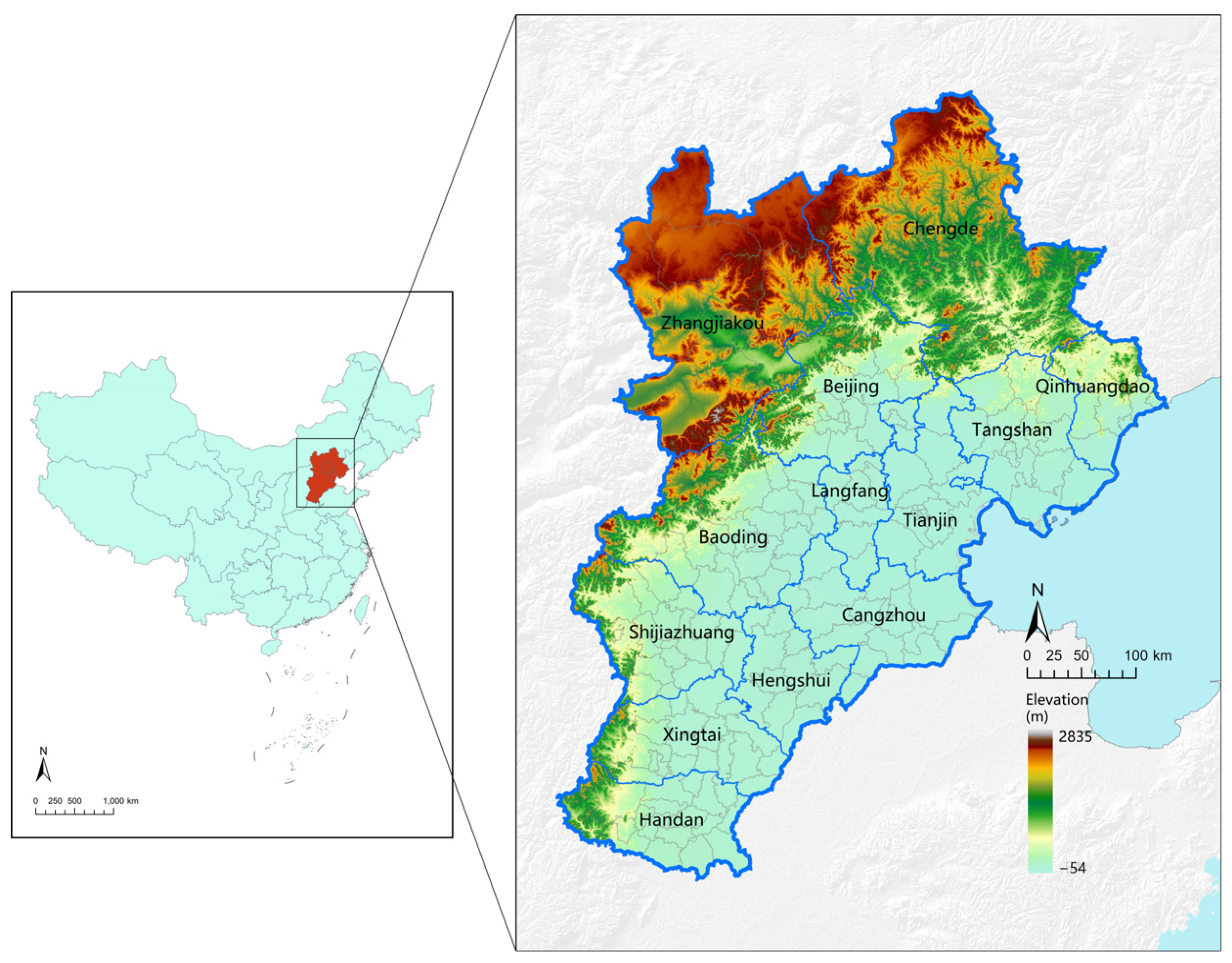
Figure 1. Geographical location of the study area.
Land 13 00554 g001
Figure 2. Workflow of this study.
Land 13 00554 g002
Figure 3. Land use patterns under the (a) ND scenario and (b) EP scenario in 2035.
Land 13 00554 g003
Figure 4. Spatial distributions of carbon emissions under the (a) ND scenario and (b) EP scenario in 2035.
Land 13 00554 g004
Figure 5. ESC under the (a) ND scenario and (b) EP scenario in 2035.
Land 13 00554 g005
Figure 6. Carbon emission networks under the LCD scenario in the BTH urban agglomeration.
Land 13 00554 g006
Figure 7. Carbon emission network in the BTH urban agglomeration: (a) indegree centrality, (b) outdegree centrality, (c) betweenness centrality, (d) out-closeness centrality, and (e) in-closeness centrality.
Land 13 00554 g007
Figure 8. Flowchart of carbon balance zoning planning.
Land 13 00554 g008
Figure 9. Flowchart of key carbon balance and county planning.
Land 13 00554 g009
Figure 10. Carbon balance zoning and key county planning for the BTH urban agglomeration in 2035 under the LCD scenario.
Land 13 00554 g010
Figure 11. Key regional proposals for emission peak and carbon neutrality engineering for the BTH urban agglomeration in 2035 under the LCD scenario.
Land 13 00554 g011
Figure 12. A low-carbon-oriented urban agglomeration planning framework.
Land 13 00554 g012
Table 1. Details of the datasets.
Data TypesData YearsSpatial Resolution (m)Sources
Land use datasetsLand use2000, 2010, 202030Jie Yang and Xin Huang (2022). The 30 m annual land-cover dataset and its dynamics in China from 1990 to 2021 [Dataset]. In Earth System Science Data (1.0.1, Vol. 13, Number 1, pp. 3907–3925). Zenodo. https://doi.org/10.5281/zenodo.5816591 [24]
Climate environmental datasetsSoil type201830Resource and Environmental Sciences Data Center, Chinese Academy of Sciences
Annual mean temperature202030National Tibetan Plateau Data Center
Annual mean precipitation202030National Tibetan Plateau Data Center
DEM202030Geospatial Data Cloud
Slope 202030Generated from DEM data using ArcGIS
Socioeconomic datasetsGDP20191000Resource and Environmental Sciences Data Center, Chinese Academy of Sciences
POP20191000Resource and Environmental Sciences Data Center, Chinese Academy of Sciences
Proximity to railway202030Open street map
Proximity to motorway202030Open street map
Proximity to national highway202030Open street map
Proximity to river water202030Open street map
Nighttime light data20201000Chinese Long Time Series Nighttime Light Dataset of China (2000–2020)
https://doi.org/10.3974/geodb.2022.06.01.V1 [25]
Future driver datasetNational nature reserves//China Nature Reserve Specimen Resource Sharing
Table 2. Carbon emission coefficients of different land use types.
Land Use TypesCoefficient (ton CO2/hm2)References
Cultivated land0.42Fang et al., 2007 [29], She et al., 2017 [31]
Forest−0.62Fang et al., 2007 [29], Cui et al., 2019 [28]
Grassland−0.14Fang et al., 2007 [29], Cui et al., 2019 [28]
Shrub−0.23Tang et al., 2018 [32], Cui et al., 2019 [28]
Waterbody−0.03Fang et al., 2007 [29], Cui et al., 2019 [28]
Built-up land120.37Liu et al., 2023 [30], Yan et al., 2022 [33]
Unused land−0.05Cui et al., 2019 [28]
Table 3. Spatial network indicators of carbon emissions.
Network CharacteristicsFormulaSymbolic MeaningRole
Degree of CentralityOutdegree Centrality C o d i = j = 1 n X i j / n 1 X indicates whether there is a direct connection between counties, where 1 indicates a direct connection and 0 indicates no connection; n is the number of cities in the networkDirectly reflects the status of nodes in the network
Indegree Centrality C i d i = j = 1 n X j i / n 1
Closeness of CentralityIn-closeness
Centrality
C i c i = n 1 / Σ j = 1 n d j , i d i , j denotes the shortest spherical distance from county i to county j Reflects the degree to which each city in the entire network is not dominated by the other cities
Out-closeness
Centrality
C o c i = n 1 / Σ j = 1 n d i , j
Betweenness Centrality C b i = Σ j < k g j k i / g j k n 1 n 2 g j k represents the total number of shortest paths from county j to county k that generate links; g j k i is the number of shortest paths from county j to county k that generate links through county i Reflects the extent to which a node can control the relationships between other nodes
Table 4. Comparison between the simulated land use types and the actual land use types in 2020 at pixel level.
Cultivated LandForestShrubGrasslandWaterbodyUnused LandBuilt-Up Land
Real (2020)472,275265,4623252160,05515,016265160,376
Simulation
results (2020)
472,401265,3383226159,87414,225282161,355
Table 5. Changes in the regional area under different scenarios in 2020–2025 (ha).
YearScenario AnalysisCultivated LandForestShrubGrasslandWaterbodyUnused LandBuilt-Up Land
2020 9,433,1285,314,13963,9303,189,193281,33046523,224,288
2035ND9,236,8935,565,08258,0232,909,005299,49220863,440,079
EP9,061,2655,639,40856,8563,059,093303,33829053,387,795
2020–2035ND−196,235250,943−5907−280,18818,162−2566215,791
EP−371,863325,269−7074−130,10022,008−1747163,507
Table 6. Carbon emissions under the ND scenario and EP scenario in 2035 (104 t).
Scenario AnalysisCultivated LandForestShrubGrasslandWaterbodyUnused LandBuilt-Up Land
ND387.95−345.04−1.33−40.73−0.90−0.0141,408.23
EP380.57−349.64−1.31−42.83−0.91−0.0140,778.89
Table 7. Number of counties in the top 10% of the centrality indicators for each city.
Degree of CentralityCloseness of CentralityBetweenness of
Centrality
Outdegree CentralityIndegree
Centrality
Out-Closeness
Centrality
In-Closeness
Centrality
CitiesNo.CitiesNo.CitiesNo.CitiesNo.CitiesNo.
Chengde6Beijing10Hengshui8Tianjin9Baoding4
Baoding4Tianjin8Baoding6Beijing8Beijing4
Cangzhou4Baoding1Cangzhou4Baoding2Cangzhou3
Hengshui4Shijiazhuang1Shijiazhuang1Cangzhou1Hengshui3
Zhangjiakou2 Zhangjiakou1 Tianjin3
Langfang1
Shijiazhuang1
Xingtai1
Table 8. Carbon balance zoning planning for the BTH urban agglomeration in 2035 under the LCD scenario.
Carbon-Balance ZoningDivision CriteriaFunctional Features
Ecological
conservation area
ESC > 1, belongs to the carbon emission linkage areaThe ecological conservation area primarily resided in the northwestern region of the Beijing–Tianjin–Tangshan–Baoding–Cangzhou carbon emission linkage area. It accounted for 4.699% of the urban agglomeration area. The region has strong carbon sink capacity and is situated within the carbon emission linkage area, so it can give full play to the carbon sink regulation capacity of the ecological region and drive the overall coordinated emission reduction within the carbon emission network.
Carbon sink
balance area
ESC > 1, does not belong to the
carbon emission linkage area
The carbon sink balance area was located mainly in the northwestern part of Hebei Province. It accounted for 43.322% of the urban agglomeration area and was composed mainly of 33 counties. The region has a strong ecological function, high carbon sink benefit, and low carbon emissions, so it is suitable to introduce economically developed county industries appropriately and continue to carry out ecological environmental construction.
Carbon emission linkage control areaESC ≤ 1, belongs to the carbon emission linkage areaThe carbon emission linkage control area was composed mainly of counties in three carbon emission linkage areas. It accounted for 22.207% of the urban agglomeration area and was composed mainly of 87 counties. The region exhibits significant carbon emissions and is integrated into the carbon emission network, enabling it to effectively utilize the influence mechanism of the carbon emission network and establish a regional carbon emission reduction linkage system [20].
Low-carbon control areaESC ≤ 1, does not belong to the
carbon emission linkage area
The low-carbon control area was located mainly in the central and southern parts of the urban agglomeration. It accounted for 25.369% of the urban agglomeration area and was composed of 74 counties. The region has high carbon emissions, but it has less contact with other counties in the BTH region and is difficult for the other counties to affect. It is necessary to strengthen communication with other regions and gradually carry out project cooperation and technical exchanges with provinces and cities.
Table 9. Planning of key counties for carbon balance in 2035 under the LCD scenario in the BTH urban agglomeration.
County TypeDivision CriteriaFunctional Features
Core countyCounties with higher indegree centralityThese counties dominate the central position within the carbon emission network, deserving top priority in shaping regional policies for carbon emission reduction. The optimization of socioeconomic development and energy development top-level design in these core counties is essential. The construction of a carbon emission trading market should be strengthened with market-oriented low-carbon mechanisms.
Promotion countyCounties with higher in-closeness centralityCounties that are more connected to other counties can change their car-bon emission behaviors and the carbon emission behaviors of their neighboring counties more quickly, so they should be used as promotion counties for carbon emission reduction and sink increase, further promoting emission peak and carbon neutrality policies according to local conditions. The government can learn from the experience of advanced cities to promote the effective implementation of coordinated emission reduction planning.
Bridge countyCounties with higher betweenness centralityCounties that play a communication role in the network can control the coordinated emission reduction process in other cities in a planned manner. These counties provide network communication and can carry out key planning control. By limiting some functions, the government can minimize the exchange of ineffective carbon emissions, impede unnecessary carbon emission connections.
Improvement countyCounties with higher outdegree centralityThese counties exhibit a greater number of spatial spillover relationships within the carbon emission network and bear a higher burden of carbon emissions. Their ecological conservation function is strong, and their spillover effect can be used to carry out ecological environmental construction and avoid ecological degradation caused by overurbanization and industrial development.
Table 10. Key regional proposals for emission peak and carbon neutrality projects in the BTH urban agglomeration in 2035 under LCD scenarios.
Region
Type
Prefecture
-Level City
CountyCarbon Balance
Zoning
County TypeKey Areas for Emission Peak and Carbon Neutrality Projects
Single CountyBeijingFangshan DistrictEcological Conservation AreaExtension County,
Bridge County
Carbon reduction: Yanfang, Liangxiang, Doudian, three high-tech clusters
Sink enhancement: Juma River Basin, Shidu Scenic Spot, Shihua Cave Scenic Spot, Baicao Riverside Scenic Spot, Yongding River Forest Wetland Leisure Belt.
BeijingHaidian DistrictCarbon Emission Linkage Control AreaCore County,
Promotion County
Carbon reduction: Zhongguancun Science City
Sink enhancement: Xishan Ecological Barrier, Green Heart of Three Hills and Five Gardens, Green Heart of Ecological Science and Technology.
ChengdePingquan CityCarbon Sink Balance AreaImprovement CountySink enhancement: ecological protection of Liaoheyuan Forest Ecological Reserve, Shihu Forest Park, Qinghe Forest Park, Yamenzi Forest Park, Shuangfengshan Forest Park, Shanwanzi Forest Park, Longtanshan Forest Park, Pu River Waterfront Ecological Corridor.
CangzhouHejian CityLow-Carbon
Control Area
Improvement County,
Bridge County
Carbon reduction: central urban area and eastern cluster
Sink enhancement: Nine River System (referring to the nine main rivers in the city, including east branch of Xiaobai River, Yujia River, Guyang River, east branch of Ren River, west branch of Ren River, Ziya River, Beipai River, and west branch of Heilonggang River).
Cross-
Regional Cooperation
HengshuiTaocheng District, Jizhou DistrictCarbon Emission Linkage Control Area,
Low-Carbon
Control Area
Bridge CountyCarbon reduction: National Demonstration Zone for Transformation of Scientific and Technological Achievements to the south of Beijing, Hengshui High-Tech Industry Development Zone, Taocheng High-Tech Industry Development Zone, and Jizhou High-Tech Industry Development Zone
Sink enhancement: Hengshui Lake National Nature Reserve, Fuyang River Water Ecological Comprehensive Renovation Area, Taocheng Urban Area–Binhu New Area and Jizhou Urban Area Blue and Green Space System, Fuyang New River–Fudong Pai River Flood Discharge Corridor, Fuyang River, and Yanhe Old Course.
Zhangjiakou–
Baoding–
Beijing
Yu county,
Zhuolu County, Laishui County, Mentougou District, Fangshan District
Carbon Sink Balance Area,
Ecological Conservation Area
Bridge County,
Promotion County,
Improvement County
Sink enhancement:
Important water ecological corridor: Mentougou District–Fangshan District–Yu County–Zhuolu County: Yongding River Basin (Zhangjiakou Section)
Laishui County–Fangshan District: Water Source Protection Area of Juma River Basin
Important nature reserves:
Yu County–Zhuolu County: Xiaowutai Mountain National Forest Ecological Reserve in Hebei Province
Zhuolu County–Laishui County: Jinhua Mountain–Henglingzi Crossoptilon Mantchuricum Nature Reserve
Mentougou District–Fangshan District: Beijing Baihuashan National Forest Ecological Reserve.
Disclaimer/Publisher’s Note: The statements, opinions and data contained in all publications are solely those of the individual author(s) and contributor(s) and not of MDPI and/or the editor(s). MDPI and/or the editor(s) disclaim responsibility for any injury to people or property resulting from any ideas, methods, instructions or products referred to in the content.